跳到论文正文
W Papers独立论文阅读器 arXiv:1602.04660 论文正文 计算阅读时间 · 0%
引用这篇论文根据当前论文元数据生成,正式投稿前建议核对。


License: arXiv.org perpetual non-exclusive license
arXiv:1602.04660v1 [q-fin.MF] 15 Feb 2016

Bayesian Dividend Optimization and Finite Time Ruin Probabilities

Gunther Leobacher    Michaela Szölgyenyi ††thanks: The author is supported by the Austrian Science Fund (FWF) Project P21943.    Stefan Thonhauser ††thanks: Stefan Thonhauser is supported by Swiss National Science Foundation (SNF) Project 200021-124635/1.
January 2014
Abstract

We consider the valuation problem of an (insurance) company under partial information. Therefore we use the concept of maximizing discounted future dividend payments. The firm value process is described by a diffusion model with constant and observable volatility and constant but unknown drift parameter. For transforming the problem to a problem with complete information, we derive a suitable filter. The optimal value function is characterized as the unique viscosity solution of the associated Hamilton-Jacobi-Bellman equation. We state a numerical procedure for approximating both the optimal dividend strategy and the corresponding value function. Furthermore, threshold strategies are discussed in some detail. Finally, we calculate the probability of ruin in the uncontrolled and controlled situation.

Keywords: dividend maximization, stochastic optimal control, filtering theory, viscosity solutions, finite time ruin probabilities
Mathematics Subject Classification (2010): 49L20, 91B30, 93E20

M. Szölgyenyi 🖂
Department of Financial Mathematics, Johannes Kepler University Linz, 4040 Linz, Austria
michaela.szoelgyenyi@jku.at

G. Leobacher
Department of Financial Mathematics, Johannes Kepler University Linz, 4040 Linz, Austria

S. Thonhauser
Department of Actuarial Science, University of Lausanne, 1015 Lausanne, Switzerland

1 Introduction

In this paper we are going to study the valuation problem of an (insurance) company. We assume that the firm value process is given by a Brownian motion with drift, and is absorbed when hitting zero. In contrast to existing results, the drift parameter is modeled as an unobservable Bernoulli-type random variable and the company can only observe the evolution of its firm value.
In an insurance context de Finetti [6] proposed the expected discounted future dividend payments as a valuation principle for a homogeneous insurance portfolio. However, one can extend this concept to large companies, not necessarily being insurers. The accumulated dividends are described by an absolutely continuous process such that the company is capable of controlling its dividend rate with the aim of maximizing the expected value of accumulated discounted dividend payments.
In mathematical terms we face the problem of determining

supu∈A𝔼x​(∫0τe−δ​t​ut​𝑑t),\displaystyle\sup_{u\in A}{\mathbb{E}}_{x}\left(\int_{0}^{\tau}e^{-\delta t}u_{t}\,dt\right)\,,

where the controlled firm value, controlled by some dividend rate (ut)t≥0(u_{t})_{t\geq 0}, and lifetime are given by

Xt\displaystyle X_{t} =x+θ​t+σ​Bt−∫0tus​𝑑s,\displaystyle=x+\theta t+\sigma B_{t}-\int_{0}^{t}u_{s}\,ds\,,
τ\displaystyle\tau =inf{t≥0|Xt≤0}.\displaystyle=\inf\{t\geq 0\,|\,X_{t}\leq 0\}\,.

The drift parameter is a random variable θ∈{θ1,θ2}\theta\in\{\theta_{1},\theta_{2}\} with known distribution. In this so-called Bayesian framework the company can only observe the wealth process and thus faces an optimal control problem under partial information. The a-priori unknown drift parameter expresses the company’s uncertainty on the profitability of some business activities or an uncertainty on the general economic environment in addition to the basic risk represented by the Brownian component.

In the insurance context the unknown drift parameter can be interpreted as a residual uncertainty when using a diffusion approximation of a classical risk reserve process instead of the original model. For diffusion models with observable parameters this problem and several variants of it have been studied intensively, for example by Shreve et al. [27], Jeanblanc-Piqué and Shiryaev [14], Radner and Shepp [23], and Asmussen and Taksar [2]. For an overview, the interested reader may consult Schmidli [26], Albrecher and Thonhauser [1], or Avanzi [3]. Two recent papers, Jiang and Pistorius [15], and Sotomayor and Cadenillas [28] deal with the dividend problem under a changing economic environment, described by parameters driven by an observable Markov chain. However these models still assume full information and therefore differ from the model studied here.
The dividend maximization problem is also related to a pure optimal consumption problem of an economic agent. The agent is capable of controlling his/her consumption intensity.
Papers pointing towards optimal consumption problems arising in mathematical finance are Hubalek and Schachermayer [13] and Grandits et al. [12], maximizing expected accumulated utility of dividends, and expected utility of accumulated dividends, respectively.
In corporate finance a similar problem appears, sometimes in combination with an optimal stopping problem, in liquidity risk modeling. There the firm value process corresponds to the cash reserve process of a company, the market value of shares of which is given by expected future dividend payments, for instance see Décamps and Villeneuve [7]. In this framework an uncertain drift parameter is taken up in Décamps and Villeneuve [8], where the solution of a special case of an associated singular control problem is presented.
Models with partial information - in particular hidden Markov models - appear quite frequently in the literature on portfolio optimization problems, e.g., by Karatzas and Zhao [17], Rieder and Bäuerle [24], and Sass and Haussmann [25], whereas results relating to actuarial mathematics are more scarce. Gerber [11] uses a Brownian motion with unknown drift for modeling the value of a single insurance policy, of which it is a-priori not known whether it is a good or bad risk. He answers the question of when to optimally cancel the policy, i.e., when the insurer should decide that the risk actually corresponds to a bad one. For a diffusion risk reserve process with parameters generated by a hidden Markov chain, partial differential equations associated to finite time ruin probabilities are derived by Elliott et al. [9].

The main contribution of the present paper is the complete analytical characterization of the solution of the dividend maximization problem under partial information. Furthermore, based on the analytical findings, we provide a numerical procedure for determining approximations of the optimal value function and dividend strategy. As a complement, following the path described by Elliott et al. [9], we consider the associated finite time ruin probabilities for the uncontrolled and the controlled situation.

The paper is organized as follows. In Section 2 we give a mathematical description of the model and the optimization problem. In Section 3 we derive, by means of filtering theory, an estimator for the unknown drift parameter to overcome uncertainty. The applicability of the dynamic programming approach and the associated Hamilton-Jacobi-Bellman (HJB) equation for the filtered optimization problem are given in Section 4. Section 5 contains the complete theoretical characterization of the optimal value function as the unique viscosity solution of the associated HJB equation. As the proofs are rather technical, they have been moved to the Appendix. In Section 6 we describe a numerical method for calculating approximations to the optimal value function and optimal dividend strategy. Section 7 deals with the special class of threshold strategies, under which dividends are paid only if the firm value process exceeds a certain threshold level. The finite time ruin probabilities are considered in Section 8. Section 9 concludes the paper.

2 Preliminaries

In the whole paper we consider a filtered probability space (ℰ,ℱ,{ℱt}t≥0,ℙ)({\cal E},{\cal F},\{{\cal F}_{t}\}_{t\geq 0},{\mathbb{P}}) carrying all stochastic quantities which will be introduced in the following.
As stated in the introduction, we assume that the firm value of a company is given by

Xt=x+∫0tθ​𝑑s+σ​Bt−Lt,X_{t}=x+\int_{0}^{t}\theta\,ds+\sigma B_{t}-L_{t}\,, (1)

with initial capital x>0x>0, where θ\theta is the constant unobservable drift, θ∈{θ1,θ2}\theta\in\{\theta_{1},\theta_{2}\}, θ1<θ2\theta_{1}<\theta_{2}, σ\sigma is the constant and known volatility, and B=(Bt)t≥0B=(B_{t})_{t\geq 0} is a standard Brownian motion. The accumulated dividend process L=(Lt)t≥0L=(L_{t})_{t\geq 0}, L0=0L_{0}=0, is assumed to admit a density u=(ut)t≥0u=(u_{t})_{t\geq 0}, which is bounded, i.e., ut∈[0,K]u_{t}\in[0,K], K>0K>0, such that

d​Lt=ut​d​t.\displaystyle dL_{t}=u_{t}\,dt\,. (2)

Note that XX always corresponds to a certain strategy uu, but for avoiding an elaborate notation, we will not make that explicit as long as it causes no ambiguities.
For modeling a further uncertainty of the company’s firm value in addition to the Brownian component we assume that it is not possible to observe the drift parameter directly, but we assume knowledge of its (initial) distribution q:=ℙ⁡(θ=θ1)=1−ℙ⁡(θ=θ2)q:={\mathbb{P}}(\theta=\theta_{1})=1-{\mathbb{P}}(\theta=\theta_{2}).
We denote the uncontrolled firm value process by Z=(Zt)t≥0Z=(Z_{t})_{t\geq 0}, which is given through

Zt\displaystyle Z_{t} =x+θ​t+σ​Bt,\displaystyle=x+\theta t+\sigma B_{t}\,, (3)

and obviously Xt=Zt−LtX_{t}=Z_{t}-L_{t}. The observation filtration {ℱtZ}t≥0\{{\cal F}^{Z}_{t}\}_{t\geq 0} is the augmentation of the filtration generated by ZZ. This means that the company is able to observe the evolution of its uncontrolled firm value and based on that decides on the dividend strategy, or equivalently observes controlled firm value and accumulated dividends.

The value process associated with a dividend strategy uu is defined as

Jt(u):=𝔼⁡(∫tτe−δ⁡(s−t)​us​𝑑s​ℱtZ),J_{t}^{(u)}:={\mathbb{E}}\left(\int_{t}^{\tau}e^{-\delta(s-t)}u_{s}\,ds\,\vline\,{\cal F}_{t}^{Z}\right)\,,

where τ:=inf{s≥tXs≤0}\tau:=\inf\{s\geq t\,\vline\,X_{s}\leq 0\} is the time of ruin of XX for the corresponding dividend strategy uu. τ\tau depends on the strategy uu via XX, and again we will not make this explicit if there is no danger of confusion.
The optimal value process of the optimization problem under study is given by

Vt=supu∈A𝔼⁡(∫tτe−δ⁡(s−t)​us​𝑑s​ℱtZ),V_{t}=\sup_{u\in A}{\mathbb{E}}\left(\int_{t}^{\tau}e^{-\delta(s-t)}u_{s}\,ds\,\vline\,{\cal F}_{t}^{Z}\right)\,,

where AA denotes the set of admissible controls, for which we take the set of all {ℱtZ}t≥0\{{\cal F}^{Z}_{t}\}_{t\geq 0}-progressively measurable and [0,K][0,K]-valued processes. Naturally, an optimal strategy u∗u^{*} is characterized by Vt=Jt(u∗)V_{t}=J_{t}^{(u^{*})}.

Since we cannot observe the two sources θ\theta and BtB_{t} of uncertainty separately, we face a stochastic optimization problem under partial information. For overcoming this difficulty we are going to derive an observable estimator for the drift parameter by means of filtering theory in the following section.

3 Filtering theory

Our aim is to rewrite (1) as

Xt=x+∫0t(θs−us)​𝑑s+σ​Wt,X_{t}=x+\int_{0}^{t}(\theta_{s}-u_{s})\,ds+\sigma W_{t}\,, (4)

where (θt)t≥0(\theta_{t})_{t\geq 0} is an observable estimator for θ\theta at time tt and (Wt)t≥0(W_{t})_{t\geq 0} is a Brownian motion w.r.t. our observation filtration.

Remark 3.1.

In Liptser and Shiryaev [21, p. 225] the maximum likelihood estimator for the unknown drift parameter in the present situation is given by θ^t=Zt−zt\hat{\theta}_{t}=\frac{Z_{t}-z}{t}. One may notice that this estimator only uses the information which is given by ZtZ_{t} and does not consider the whole path up to time tt. In the following we are going to derive an alternative estimator for θ\theta which is based on an application of Bayes’ rule. This estimator obeys an appealing representation in terms of a stochastic integral and induces natural boundary conditions for the optimization problem.

Using

ℙ⁡(Zt∈[z¯,z¯+d​z¯]|θ=θj)=12​π​σ​t​exp⁡(−(z¯−θj​t−z)22​σ2​t)​d​z,{\mathbb{P}}(Z_{t}\in[\bar{z},\bar{z}+d\bar{z}]|\theta=\theta_{j})=\frac{1}{\sqrt{2\pi}\sigma\sqrt{t}}\exp\left(-\frac{(\bar{z}-\theta_{j}t-z)^{2}}{2\sigma^{2}t}\right)\,dz\,,

and the law of total probability we arrive at

ℙ⁡(Zt∈[z¯,z¯+d​z¯])=(q​12​π​σ​t​exp⁡(−(z¯−θ1​t−z)22​σ2​t)+(1−q)​12​π​σ​t​exp⁡(−(z¯−θ2​t−z)22​σ2​t))​d​z.\displaystyle{\mathbb{P}}(Z_{t}\in[\bar{z},\bar{z}+d\bar{z}])=\left(q\frac{1}{\sqrt{2\pi}\sigma\sqrt{t}}\exp\left(-\frac{(\bar{z}-\theta_{1}t-z)^{2}}{2\sigma^{2}t}\right)+(1-q)\frac{1}{\sqrt{2\pi}\sigma\sqrt{t}}\exp\left(-\frac{(\bar{z}-\theta_{2}t-z)^{2}}{2\sigma^{2}t}\right)\right)\,dz\,.

Now Bayes’ theorem allows us to determine

ℙ⁡(θ=θ1​Zt∈[z¯,z¯+d​z¯])\displaystyle{\mathbb{P}}(\theta=\theta_{1}\,\vline\,Z_{t}\in[\bar{z},\bar{z}+d\bar{z}]) =q​12​π​σ​t​exp⁡(−(z¯−θ1​t−z)22​σ2​t)​d​z(q​12​π​σ​t​exp⁡(−(z¯−θ1​t−z)22​σ2​t)+(1−q)​12​π​σ​t​exp⁡(−(z¯−θ2​t−z)22​σ2​t))​d​z\displaystyle=\frac{q\frac{1}{\sqrt{2\pi}\sigma\sqrt{t}}\exp\left(-\frac{(\bar{z}-\theta_{1}t-z)^{2}}{2\sigma^{2}t}\right)\,dz}{\left(q\frac{1}{\sqrt{2\pi}\sigma\sqrt{t}}\exp\left(-\frac{(\bar{z}-\theta_{1}t-z)^{2}}{2\sigma^{2}t}\right)+(1-q)\frac{1}{\sqrt{2\pi}\sigma\sqrt{t}}\exp\left(-\frac{(\bar{z}-\theta_{2}t-z)^{2}}{2\sigma^{2}t}\right)\right)\,dz}
=11+1−qq​exp⁡((θ2−θ1)​(z¯−z−12​(θ1+θ2)​t)σ2),\displaystyle=\frac{1}{1+\frac{1-q}{q}\exp\left(\frac{(\theta_{2}-\theta_{1})(\bar{z}-z-\frac{1}{2}(\theta_{1}+\theta_{2})t)}{\sigma^{2}}\right)}\,,

and to compute θt=𝔼⁡(θ​Zt∈[z¯,z¯+d​z¯])\theta_{t}={\mathbb{E}}(\theta\,\vline\,Z_{t}\in[\bar{z},\bar{z}+d\bar{z}]). Setting θt=h⁡(t,Zt)\theta_{t}=h(t,Z_{t}), we finally get

h⁡(t,z¯)=θ1​11+f⁡(t,z¯)+θ2​f⁡(t,z¯)1+f⁡(t,z¯)=θ1+(θ2−θ1)​f⁡(t,z¯)1+f⁡(t,z¯),\displaystyle h(t,\bar{z})=\theta_{1}\frac{1}{1+f(t,\bar{z})}+\theta_{2}\frac{f(t,\bar{z})}{1+f(t,\bar{z})}=\theta_{1}+(\theta_{2}-\theta_{1})\frac{f(t,\bar{z})}{1+f(t,\bar{z})}\,,
f⁡(t,z¯)=1−qq​exp⁡((θ2−θ1)​(z¯−z−12​(θ1+θ2)​t)σ2).\displaystyle f(t,\bar{z})=\frac{1-q}{q}\exp\left(\frac{(\theta_{2}-\theta_{1})(\bar{z}-z-\frac{1}{2}(\theta_{1}+\theta_{2})t)}{\sigma^{2}}\right)\,.

As a consequence we can state the following Lemma.

Lemma 3.2.

ZtZ_{t} and θt\theta_{t} are connected via

Zt=σ2​log⁡(θt−θ1)​q(θ2−θt)​(1−q)(θ2−θ1)+z+12​(θ1+θ2)​t.Z_{t}=\frac{\sigma^{2}\log\frac{(\theta_{t}-\theta_{1})q}{(\theta_{2}-\theta_{t})(1-q)}}{(\theta_{2}-\theta_{1})}+z+\frac{1}{2}(\theta_{1}+\theta_{2})t\,. (5)

In particular, (θt)t≥0(\theta_{t})_{t\geq 0} is adapted to the observation filtration.

From Liptser and Shiryaev [20, Theorem 9.1] we get that

Wt=1σ​(θ​t−∫0tθs​𝑑s)+BtW_{t}=\frac{1}{\sigma}\left(\theta t-\int_{0}^{t}\theta_{s}\,ds\right)+B_{t}

is an {ℱtZ}t≥0\{{\cal F}^{Z}_{t}\}_{t\geq 0}-Brownian motion, sometimes referred to as innovation process. Therefore we can rewrite (1) and (3) as

Xt\displaystyle X_{t} =x+∫0t(θs−us)​𝑑s+σ​Wt,\displaystyle=x+\int_{0}^{t}(\theta_{s}-u_{s})\,ds+\sigma W_{t}\,, (6)
Zt\displaystyle Z_{t} =z+∫0tθs​𝑑s+σ​Wt.\displaystyle=z+\int_{0}^{t}\theta_{s}\,ds+\sigma W_{t}\,. (7)

Due to (5), ℱtZ=ℱtX,θ{\cal F}^{Z}_{t}={\cal F}^{X,\theta}_{t} for all t≥0t\geq 0, where {ℱtX,θ}t≥0\{{\cal F}^{X,\theta}_{t}\}_{t\geq 0} is the augmented filtration generated by XX and (θt)t≥0(\theta_{t})_{t\geq 0}. Using Itô’s formula we derive (9), such that from now on we can consider the following system of state variables

Xt\displaystyle X_{t} =x+∫0t(θs−us)​𝑑s+σ​Wt,\displaystyle=x+\int_{0}^{t}(\theta_{s}-u_{s})\,ds+\sigma W_{t}\,, (8)
θt\displaystyle\theta_{t} =ϑ+1σ​∫0t(θs−θ1)​(θ2−θs)​d​Ws.\displaystyle=\vartheta+\frac{1}{\sigma}\int_{0}^{t}(\theta_{s}-\theta_{1})(\theta_{2}-\theta_{s})\,dW_{s}\,. (9)
Remark 3.3.

Let uu be any progressively measurable bounded process. Equation (9) does not depend on uu and therefore has a solution by the well-known theorem on existence and uniqueness of solutions of SDEs with Lipschitz coefficients. See, for example, Krylov [18, Chapter 2, Theorem 7].

XX does not appear on the right hand side of (8), so this becomes just an ordinary integral.

4 The Hamilton-Jacobi-Bellman equation

In this section we will show that the dynamic programming approach is applicable for solving the optimization problem when considering (Xt,θt)(X_{t},\theta_{t}) as state variables.
Remember the definition of the optimal value process

Vt:=supu∈A𝔼⁡(∫tτe−δ⁡(s−t)​us​𝑑s​ℱtZ)=supu∈A𝔼⁡(∫tτe−δ⁡(s−t)​us​𝑑s​ℱtX,θ).V_{t}:=\sup_{u\in A}{\mathbb{E}}\left(\int_{t}^{\tau}e^{-\delta(s-t)}u_{s}\,ds\,\vline\,{\cal F}_{t}^{Z}\right)=\sup_{u\in A}{\mathbb{E}}\left(\int_{t}^{\tau}e^{-\delta(s-t)}u_{s}\,ds\,\vline\,{\cal F}_{t}^{X,\theta}\right)\,.

The system (8) and (9) describes autonomous state dynamics in the sense of [10, Section IV.5]. It is therefore natural to consider Markov controls in the following. Furthermore, due to the Markovian structure and the infinite horizon, we get that

Vt\displaystyle V_{t} =supu∈A𝔼⁡(∫tτe−δ⁡(s−t)​us​𝑑s​ℱtX,θ)=supu∈A𝔼⁡(∫tτe−δ⁡(s−t)​us​𝑑s​Xt,θt)=V⁡(Xt,θt),\displaystyle=\sup_{u\in A}{\mathbb{E}}\left(\int_{t}^{\tau}e^{-\delta(s-t)}u_{s}\,ds\,\vline\,{\cal F}^{X,\theta}_{t}\right)=\sup_{u\in A}{\mathbb{E}}\left(\int_{t}^{\tau}e^{-\delta(s-t)}u_{s}\,ds\,\vline\,X_{t},\theta_{t}\right)=V(X_{t},\theta_{t})\,,

a.s., where from now on τ:=inf{t≥0Xt≤0}\tau:=\inf\{t\geq 0\,\vline\,X_{t}\leq 0\} and

V(x,ϑ):=supu∈A𝔼(∫0τe−δ​susdsX0=x,θ0=ϑ)V(x,\vartheta):=\sup_{u\in A}{\mathbb{E}}\left(\int_{0}^{\tau}e^{-\delta s}u_{s}\,ds\,\vline\,X_{0}=x,\theta_{0}=\vartheta\right)

denotes the optimal value function of the optimization problem. For a strategy u∈Au\in A we define

J(u)(x,y):=𝔼(∫0τe−δ​susdsX0=x,θ0=ϑ).J^{(u)}(x,y):={\mathbb{E}}\left(\int_{0}^{\tau}e^{-\delta s}u_{s}\,ds\,\vline\,X_{0}=x,\theta_{0}=\vartheta\right)\,.

From now on we abbreviate the expectation given the initial values X0=xX_{0}=x and θ0=ϑ\theta_{0}=\vartheta by 𝔼x,ϑ{\mathbb{E}}_{x,\vartheta}.

Remark 4.1.

From Krylov [18, Chapter 3, Theorem 5] we know that the optimal value function VV is continuous.

Lemma 4.2.

We have 0≤V≤Kδ0\leq V\leq\frac{K}{\delta} and limx→∞V⁡(x,ϑ)=Kδ\lim_{x\to\infty}V(x,\vartheta)=\frac{K}{\delta} uniformly in ϑ\vartheta. Furthermore, VV is increasing in both parameters.

Proof.

Clearly, 0≤V⁡(x,ϑ)≤∫0∞K​e−δ​s​𝑑s=Kδ0\leq V(x,\vartheta)\leq\int_{0}^{\infty}Ke^{-\delta s}ds=\frac{K}{\delta}. On the other hand, we have V⁡(x,ϑ)≥𝔼x,ϑ​(∫0τe−δ​t​K​𝑑t)V(x,\vartheta)\geq{\mathbb{E}}_{x,\vartheta}(\int_{0}^{\tau}e^{-\delta t}K\,dt), where

(X0,θ0)\displaystyle(X_{0},\theta_{0}) =(x,ϑ),\displaystyle=(x,\vartheta)\,,
d​Xt\displaystyle dX_{t} =(θt−K)​d​t+σ​d​Wt,\displaystyle=(\theta_{t}-K)dt+\sigma dW_{t}\,,
d​θt\displaystyle d\theta_{t} =1σ​(θt−θ1)​(θ2−θt)​d​Wt,\displaystyle=\frac{1}{\sigma}(\theta_{t}-\theta_{1})(\theta_{2}-\theta_{t})dW_{t}\,,
τ\displaystyle\tau =inf{t≥0Xt≤0}.\displaystyle=\inf\{t\geq 0\,\vline\,X_{t}\leq 0\}\,.

Since we always assume θ1<θ2\theta_{1}<\theta_{2},

Xt=x+∫0t(θs−K)​𝑑s+σ​Wt≥x+∫0t(θ1−K)​𝑑s+σ​Wt=:XtminX_{t}=x+\int_{0}^{t}(\theta_{s}-K)\,ds+\sigma W_{t}\geq x+\int_{0}^{t}(\theta_{1}-K)\,ds+\sigma W_{t}=:X^{\min}_{t}

and therefore τmin:=inf{t≥0Xtmin≤0}≤τ\tau^{\min}:=\inf\{t\geq 0\,\vline\,X^{\min}_{t}\leq 0\}\leq\tau such that

V⁡(x,ϑ)≥𝔼x,ϑ​(∫0τmine−δ​t​K​𝑑t)=Kδ​(1−𝔼x,ϑ​(e−δ​τmin)).V(x,\vartheta)\geq{\mathbb{E}}_{x,\vartheta}\left(\int_{0}^{\tau^{\min}}e^{-\delta t}K\,dt\right)=\frac{K}{\delta}\left(1-{\mathbb{E}}_{x,\vartheta}\left(e^{-\delta\tau^{\min}}\right)\right)\,.

The last expectation can be computed using standard techniques: for every λ>0\lambda>0 the process defined by Mt:=e−λ​Wt−λ22​tM_{t}:=e^{-\lambda W_{t}-\frac{\lambda^{2}}{2}t} is a martingale and the stopped process MτminM^{\tau^{\min}} is a bounded martingale, such that 𝔼x,ϑ​(eλ​x+(θ1−K)​τminσ−λ22​τmin)=𝔼x,ϑ​(e−λ​Wτmin−λ22​τmin)=1{\mathbb{E}}_{x,\vartheta}(e^{\lambda\frac{x+(\theta_{1}-K)\tau^{\min}}{\sigma}-\frac{\lambda^{2}}{2}{\tau^{\min}}})={\mathbb{E}}_{x,\vartheta}(e^{-\lambda W_{\tau^{\min}}-\frac{\lambda^{2}}{2}{\tau^{\min}}})=1, and hence 𝔼x,ϑ​(eλ⁡((θ1−K)σ−λ2)​τmin)=e−λ​xσ{\mathbb{E}}_{x,\vartheta}(e^{\lambda(\frac{(\theta_{1}-K)}{\sigma}-\frac{\lambda}{2}){\tau^{\min}}})=e^{-\lambda\frac{x}{\sigma}}. We therefore get 𝔼x,ϑ​(e−δ​τmin)=e−λ​x{\mathbb{E}}_{x,\vartheta}\left(e^{-\delta\tau^{\min}}\right)=e^{-\lambda x}\,, where

λ:=(θ1−K)+(θ1−K)2+2​δ​σ2σ2.\lambda:=\frac{(\theta_{1}-K)+\sqrt{(\theta_{1}-K)^{2}+2\delta\sigma^{2}}}{\sigma^{2}}\,. (10)

The monotonicity of VV with respect to both parameters follows from a pathwise argument similar to that above. Thereby one has to keep in mind the assumption θ1<θ2\theta_{1}<\theta_{2}. ∎

Formally applying Itô’s formula to VV gives

d​V​(Xt,θt)\displaystyle dV(X_{t},\theta_{t}) =Vx​d​Xt+12​Vx​x​(d​Xt)2+Vx​ϑ​d​Xt​d​θt+Vϑ​d​θt+12​Vϑ​ϑ​(d​θt)2\displaystyle=V_{x}dX_{t}+\frac{1}{2}V_{xx}(dX_{t})^{2}+V_{x\vartheta}dX_{t}d\theta_{t}+V_{\vartheta}d\theta_{t}+\frac{1}{2}V_{\vartheta\vartheta}(d\theta_{t})^{2}
=(θt−ut)​Vx​d​t+σ​Vx​d​Wt+σ22​Vx​x​d​t+(θt−θ1)​(θ2−θt)​Vx​ϑ​d​t\displaystyle=(\theta_{t}-u_{t})V_{x}dt+\sigma V_{x}\,dW_{t}+\frac{\sigma^{2}}{2}V_{xx}\,dt+(\theta_{t}-\theta_{1})(\theta_{2}-\theta_{t})V_{x\vartheta}\,dt
+(θt−θ1)​(θ2−θt)σ​Vϑ​d​Wt+12​σ2​(θt−θ1)2​(θ2−θt)2​Vϑ​ϑ​d​t\displaystyle+\frac{(\theta_{t}-\theta_{1})(\theta_{2}-\theta_{t})}{\sigma}V_{\vartheta}\,dW_{t}+\frac{1}{2\sigma^{2}}(\theta_{t}-\theta_{1})^{2}(\theta_{2}-\theta_{t})^{2}V_{\vartheta\vartheta}\,dt
=:ℒ​V​(Xt,θt)​d​t−ut​Vx​d​t+(σ​Vx+(θt−θ1)​(θ2−θt)σ​Vϑ)​d​Wt.\displaystyle=:{\cal L}V(X_{t},\theta_{t})\,dt-u_{t}V_{x}dt+\left(\sigma V_{x}+\frac{(\theta_{t}-\theta_{1})(\theta_{2}-\theta_{t})}{\sigma}V_{\vartheta}\right)\,dW_{t}\,.

We now prove a version of the dynamic programming principle, or Bellman principle.

Proposition 4.3 (Bellman principle).

For every bounded stopping time η\eta we have

V⁡(x,ϑ)=supu∈A𝔼x,ϑ​(∫0τ∧ηe−δ​t​ut​𝑑t+e−δ⁡(τ∧η)​V​(Xτ∧η,θτ∧η)).V(x,\vartheta)=\sup_{u\in A}{\mathbb{E}}_{x,\vartheta}\left(\int_{0}^{\tau\wedge\eta}e^{-\delta t}u_{t}\,dt+e^{-\delta(\tau\wedge\eta)}V(X_{\tau\wedge\eta},\theta_{\tau\wedge\eta})\right)\,.
Proof.

Let u∗u^{*} be some ε\varepsilon-optimal strategy for (x,ϑ)(x,\vartheta), then

V⁡(x,ϑ)−ε\displaystyle V(x,\vartheta)-\varepsilon <J(u∗)​(x,ϑ)=𝔼x,ϑ​(∫0τe−δ​t​ut∗​𝑑t)\displaystyle<J^{(u^{*})}(x,\vartheta)={\mathbb{E}}_{x,\vartheta}\left(\int_{0}^{\tau}e^{-\delta t}u^{*}_{t}\,dt\right)
≤𝔼x,ϑ​(∫0τ∧ηe−δ​t​ut∗​𝑑t+e−δ⁡(τ∧η)​V​(Xτ∧η,θτ∧η))\displaystyle\leq{\mathbb{E}}_{x,\vartheta}\left(\int_{0}^{\tau\wedge\eta}e^{-\delta t}u^{*}_{t}\,dt+e^{-\delta(\tau\wedge\eta)}V(X_{\tau\wedge\eta},\theta_{\tau\wedge\eta})\right)
≤supu∈A𝔼x,ϑ​(∫0τ∧ηe−δ​t​ut​𝑑t+e−δ⁡(τ∧η)​V​(Xτ∧η,θτ∧η)),\displaystyle\leq\sup_{u\in A}{\mathbb{E}}_{x,\vartheta}\left(\int_{0}^{\tau\wedge\eta}e^{-\delta t}u_{t}\,dt+e^{-\delta(\tau\wedge\eta)}V(X_{\tau\wedge\eta},\theta_{\tau\wedge\eta})\right)\,,

which proves that V⁡(x,ϑ)≤supu∈A𝔼x,ϑ​(∫0τ∧ηe−δ​t​ut​𝑑t+e−δ⁡(τ∧η)​V​(Xτ∧η,θτ∧η))V(x,\vartheta)\leq\sup_{u\in A}{\mathbb{E}}_{x,\vartheta}\left(\int_{0}^{\tau\wedge\eta}e^{-\delta t}u_{t}\,dt+e^{-\delta(\tau\wedge\eta)}V(X_{\tau\wedge\eta},\theta_{\tau\wedge\eta})\right), since ε>0\varepsilon>0 was arbitrary.

On the other hand, for any ε>0\varepsilon>0 we have

supu∈A𝔼x,ϑ​(∫0τ∧ηe−δ​t​ut​𝑑t+e−δ⁡(τ∧η)​V​(Xτ∧η,θτ∧η))\displaystyle\sup_{u\in A}{\mathbb{E}}_{x,\vartheta}\left(\int_{0}^{\tau\wedge\eta}e^{-\delta t}u_{t}\,dt+e^{-\delta(\tau\wedge\eta)}V(X_{\tau\wedge\eta},\theta_{\tau\wedge\eta})\right)
≤𝔼x,ϑ​(∫0τ∧ηe−δ​t​ut1,ε​𝑑t+e−δ⁡(τ∧η)​J(u2,ε)​(Xτ∧η,θτ∧η))+ε,\displaystyle\leq{\mathbb{E}}_{x,\vartheta}\left(\int_{0}^{\tau\wedge\eta}e^{-\delta t}u_{t}^{1,\varepsilon}\,dt+e^{-\delta(\tau\wedge\eta)}J^{(u^{2,\varepsilon})}(X_{\tau\wedge\eta},\theta_{\tau\wedge\eta})\right)+\varepsilon\,,

where u1,εu^{1,\varepsilon} and u2,εu^{2,\varepsilon} are ε3\frac{\varepsilon}{3}-optimal and 2​ε3\frac{2\varepsilon}{3}-optimal strategies for (x,ϑ)(x,\vartheta) and (Xτ∧η,θτ∧η)(X_{\tau\wedge\eta},\theta_{\tau\wedge\eta}), respectively. From the continuity of VV one can construct these strategies by a similar procedure as stated in Azcue and Muler [4].
The concrete procedure for constructing u2,εu^{2,\varepsilon} is as follows. Fix ε>0\varepsilon>0, and determine B∈(0,∞)B\in(0,\infty) such that Kδ−V⁡(x,ϑ)<2​ε3\frac{K}{\delta}-V(x,\vartheta)<\frac{2\varepsilon}{3} for all x≥Bx\geq B. Note that for an initial value (x,ϑ)(x,\vartheta) with x≥Bx\geq B the strategy u~≡K\tilde{u}\equiv K is 2​ε3\frac{2\varepsilon}{3}-optimal.

Choose grid points x1<…<xNx_{1}<\ldots<x_{N} and ϑ1<…<ϑN\vartheta_{1}<\ldots<\vartheta_{N} such that the rectangles [xi,xi+1]×[ϑj,ϑj+1][x_{i},x_{i+1}]\times[\vartheta_{j},\vartheta_{j+1}] cover [0,B]×[θ1,θ2][0,B]\times[\theta_{1},\theta_{2}]. Since VV is increasing with each parameter, we have that

V⁡(xi,ϑj)≤V⁡(x,ϑ)≤V⁡(xi+1,ϑj+1),\displaystyle V(x_{i},\vartheta_{j})\leq V(x,\vartheta)\leq V(x_{i+1},\vartheta_{j+1})\,,

whenever (x,ϑ)∈[xi,xi+1]×[ϑj,ϑj+1](x,\vartheta)\in[x_{i},x_{i+1}]\times[\vartheta_{j},\vartheta_{j+1}]. Now, because of continuity of VV, the number NN and the grid points can be chosen such that

0≤V⁡(xi+1,ϑj+1)−V⁡(xi,ϑj)≤ε3,\displaystyle 0\leq V(x_{i+1},\vartheta_{j+1})-V(x_{i},\vartheta_{j})\leq\frac{\varepsilon}{3}\,,

for all i,ji,j. Let u~i​j\tilde{u}_{ij} be an ε3\frac{\varepsilon}{3}-optimal strategy for (xi,ϑj)(x_{i},\vartheta_{j}),

V⁡(xi,ϑj)≤J(u~i​j)​(xi,ϑj)+ε3.\displaystyle V(x_{i},\vartheta_{j})\leq J^{(\tilde{u}_{ij})}(x_{i},\vartheta_{j})+\frac{\varepsilon}{3}\,.

Note that also J(u~i​j)​(xi,ϑj)≤J(u~i​j)​(x,ϑ)≤J(u~i​j)​(xi+1,ϑj+1)J^{(\tilde{u}_{ij})}(x_{i},\vartheta_{j})\leq J^{(\tilde{u}_{ij})}(x,\vartheta)\leq J^{(\tilde{u}_{ij})}(x_{i+1},\vartheta_{j+1}).

The strategies u~i​j\tilde{u}^{ij} together with u~≡K\tilde{u}\equiv K define the strategy u2,εu^{2,\varepsilon} for (Xη∧τ,θη∧τ)(X_{\eta\wedge\tau},\theta_{\eta\wedge\tau}). For (Xη∧τ,θη∧τ)∈[xi,xi+1]×[ϑj,ϑj+1](X_{\eta\wedge\tau},\theta_{\eta\wedge\tau})\in[x_{i},x_{i+1}]\times[\vartheta_{j},\vartheta_{j+1}] we get

0\displaystyle 0 ≤V⁡(Xη∧τ,θη∧τ)−J(u~i​j)​(Xη∧τ,θη∧τ)≤V⁡(xi+1,ϑj+1)−J(u~i​j)​(xi,ϑj)\displaystyle\leq V(X_{\eta\wedge\tau},\theta_{\eta\wedge\tau})-J^{(\tilde{u}_{ij})}(X_{\eta\wedge\tau},\theta_{\eta\wedge\tau})\leq V(x_{i+1},\vartheta_{j+1})-J^{(\tilde{u}_{ij})}(x_{i},\vartheta_{j})
≤V⁡(xi,ϑj)−J(u~i​j)​(xi,ϑj)+ε3≤2​ε3.\displaystyle\leq V(x_{i},\vartheta_{j})-J^{(\tilde{u}_{ij})}(x_{i},\vartheta_{j})+\frac{\varepsilon}{3}\leq\frac{2\varepsilon}{3}\,.

Finally, we choose an ε3\frac{\varepsilon}{3}-optimal strategy u1,εu^{1,\varepsilon} for the right hand side of the dynamic programming principle, i.e.,

supu∈A𝔼x,ϑ​(∫0τ∧ηe−δ​t​ut​𝑑t)≤𝔼x,ϑ​(∫0τ∧ηe−δ​t​ut1,ε​𝑑t)+ε3.\sup_{u\in A}{\mathbb{E}}_{x,\vartheta}\left(\int_{0}^{\tau\wedge\eta}e^{-\delta t}u_{t}dt\right)\leq{\mathbb{E}}_{x,\vartheta}\left(\int_{0}^{\tau\wedge\eta}e^{-\delta t}u^{1,\varepsilon}_{t}dt\right)+\frac{\varepsilon}{3}.

Now we put everything together. For any strategy uu

𝔼x,ϑ​(∫0τ∧ηe−δ​t​ut​𝑑t+e−δ⁡(τ∧η)​V​(Xτ∧η,θτ∧η))\displaystyle{\mathbb{E}}_{x,\vartheta}\left(\int_{0}^{\tau\wedge\eta}e^{-\delta t}u_{t}dt+e^{-\delta(\tau\wedge\eta)}V(X_{\tau\wedge\eta},\theta_{\tau\wedge\eta})\right)
=𝔼x,ϑ​(∫0τ∧ηe−δ​t​ut​𝑑t)+𝔼x,ϑ​(e−δ⁡(τ∧η)​V​(Xτ∧η,θτ∧η),Xτ∧η≥B)\displaystyle={\mathbb{E}}_{x,\vartheta}\left(\int_{0}^{\tau\wedge\eta}e^{-\delta t}u_{t}dt\right)+{\mathbb{E}}_{x,\vartheta}\left(e^{-\delta(\tau\wedge\eta)}V(X_{\tau\wedge\eta},\theta_{\tau\wedge\eta});X_{\tau\wedge\eta}\geq B\right)
+∑i,j𝔼x,ϑ(e−δ⁡(τ∧η)V(Xτ∧η,θτ∧η);(Xτ∧η,θτ∧η)∈[xi,xi+1)×[ϑj,ϑj+1])\displaystyle\quad+\sum_{i,j}{\mathbb{E}}_{x,\vartheta}\left(e^{-\delta(\tau\wedge\eta)}V(X_{\tau\wedge\eta},\theta_{\tau\wedge\eta});(X_{\tau\wedge\eta},\theta_{\tau\wedge\eta})\in[x_{i},x_{i+1})\times[\vartheta_{j},\vartheta_{j+1}]\right)
≤𝔼x,ϑ​(∫0τ∧ηe−δ​t​ut1,ε​𝑑t)+ε3+𝔼x,ϑ​(e−δ⁡(τ∧η)​J(u~)​(Xτ∧η,θτ∧η),Xτ∧η≥B)\displaystyle\leq{\mathbb{E}}_{x,\vartheta}\left(\int_{0}^{\tau\wedge\eta}e^{-\delta t}u^{1,\varepsilon}_{t}dt\right)+\frac{\varepsilon}{3}+{\mathbb{E}}_{x,\vartheta}\left(e^{-\delta(\tau\wedge\eta)}J^{(\tilde{u})}(X_{\tau\wedge\eta},\theta_{\tau\wedge\eta});X_{\tau\wedge\eta}\geq B\right)
+∑i,j𝔼x,ϑ(e−δ⁡(τ∧η)J(u~i​j)(Xτ∧η,θτ∧η);(Xτ∧η,θτ∧η)∈[xi,xi+1)×[ϑj,ϑj+1])+2​ε3\displaystyle\quad+\sum_{i,j}{\mathbb{E}}_{x,\vartheta}\left(e^{-\delta(\tau\wedge\eta)}J^{(\tilde{u}_{ij})}(X_{\tau\wedge\eta},\theta_{\tau\wedge\eta});(X_{\tau\wedge\eta},\theta_{\tau\wedge\eta})\in[x_{i},x_{i+1})\times[\vartheta_{j},\vartheta_{j+1}]\right)+\frac{2\varepsilon}{3}
=J(uε)+ε≤V⁡(x,ϑ)+ε,\displaystyle=J^{(u^{\varepsilon})}+\varepsilon\leq V(x,\vartheta)+\varepsilon\,,

where

utε:={ut1,ε,t≤τ∧ηut2,ε,t>τ∧η.\displaystyle u_{t}^{\varepsilon}:=\begin{cases}u_{t}^{1,\varepsilon},&t\leq\tau\wedge\eta\\ u_{t}^{2,\varepsilon},&t>\tau\wedge\eta\,.\end{cases}

Thus we have for any uu that 𝔼x,ϑ​(∫0τ∧ηe−δ​t​ut​𝑑t+e−δ⁡(τ∧η)​V​(Xτ∧η,θτ∧η))<V⁡(x,ϑ)+ε{\mathbb{E}}_{x,\vartheta}\left(\int_{0}^{\tau\wedge\eta}e^{-\delta t}u_{t}dt+e^{-\delta(\tau\wedge\eta)}V(X_{\tau\wedge\eta},\theta_{\tau\wedge\eta})\right)<V(x,\vartheta)+\varepsilon, and therefore

supu∈A𝔼x,ϑ​(∫0τ∧ηe−δ​t​ut​𝑑t+e−δ⁡(τ∧η)​V​(Xτ∧η,θτ∧η))≤V⁡(x,ϑ)+ε.\sup_{u\in A}{\mathbb{E}}_{x,\vartheta}\left(\int_{0}^{\tau\wedge\eta}e^{-\delta t}u_{t}dt+e^{-\delta(\tau\wedge\eta)}V(X_{\tau\wedge\eta},\theta_{\tau\wedge\eta})\right)\leq V(x,\vartheta)+\varepsilon\,.

Since ε>0\varepsilon>0 was arbitrary, the proof is finished. ∎

Now, still under the assumption V∈C2V\in C^{2}, we apply the dynamic programming principle and derive

V⁡(x,ϑ)\displaystyle V(x,\vartheta) =supu∈A𝔼x,ϑ​(∫0τe−δ​t​ut​𝑑t)=supu∈A𝔼x,ϑ​(∫0τ∧ηe−δ​t​ut​𝑑t+e−δ⁡(τ∧η)​V​(Xτ∧η,θτ∧η))\displaystyle=\sup_{u\in A}{\mathbb{E}}_{x,\vartheta}\left(\int_{0}^{\tau}e^{-\delta t}u_{t}\,dt\right)=\sup_{u\in A}{\mathbb{E}}_{x,\vartheta}\left(\int_{0}^{\tau\wedge\eta}e^{-\delta t}u_{t}\,dt+e^{-\delta(\tau\wedge\eta)}V(X_{\tau\wedge\eta},\theta_{\tau\wedge\eta})\right)
=supu∈A𝔼x,ϑ​(∫0τ∧ηe−δ​t​ut​𝑑t+e−δ⁡(τ∧η)​(V⁡(x,ϑ)+∫0τ∧ηd​V​(Xt,θt)))\displaystyle=\sup_{u\in A}{\mathbb{E}}_{x,\vartheta}\left(\int_{0}^{\tau\wedge\eta}e^{-\delta t}u_{t}\,dt+e^{-\delta(\tau\wedge\eta)}\left(V(x,\vartheta)+\int_{0}^{\tau\wedge\eta}\!\!\!\!dV(X_{t},\theta_{t})\right)\right)
=supu∈A𝔼x,ϑ​(∫0τ∧ηe−δ​t​ut​𝑑t+e−δ⁡(τ∧η)​(V⁡(x,ϑ)+∫0τ∧ηℒ​V​(Xt,θt)−Vx​ut​𝑑t)).\displaystyle=\sup_{u\in A}{\mathbb{E}}_{x,\vartheta}\left(\int_{0}^{\tau\wedge\eta}e^{-\delta t}u_{t}\,dt+e^{-\delta(\tau\wedge\eta)}\left(V(x,\vartheta)+\int_{0}^{\tau\wedge\eta}\!\!\!\!{\cal L}V(X_{t},\theta_{t})-V_{x}u_{t}\,dt\right)\right)\,.

Therefore,

1−e−δ⁡(τ∧η)τ∧η​V​(x,ϑ)=supu∈A𝔼x,ϑ​(1τ∧η​∫0τ∧ηe−δ​t​ut​𝑑t+1τ∧η​∫0τ∧ηℒ​V​(Xt,θt)−Vx​ut​𝑑t),\displaystyle\frac{1-e^{-\delta(\tau\wedge\eta)}}{\tau\wedge\eta}V(x,\vartheta)=\sup_{u\in A}{\mathbb{E}}_{x,\vartheta}\left(\frac{1}{\tau\wedge\eta}\int_{0}^{\tau\wedge\eta}e^{-\delta t}u_{t}\,dt+\frac{1}{\tau\wedge\eta}\int_{0}^{\tau\wedge\eta}\!\!\!\!{\cal L}V(X_{t},\theta_{t})-V_{x}u_{t}\,dt\right)\,,

and by letting η→0\eta\rightarrow 0 we arrive at

δ​V=supu∈[0,K](u+ℒ​V−u​Vx).\delta V=\sup_{u\in[0,K]}\left(u+{\cal L}V-uV_{x}\right)\,.

Thus, the associated Hamilton-Jacobi-Bellman equation is given by

(ℒ−δ)​V+supu∈[0,K](u⁡(1−Vx))=0.\displaystyle({\cal L}-\delta)V+\sup_{u\in[0,K]}(u(1-V_{x}))=0\,. (11)

The HJB equation is a second order degenerate-elliptic PDE since there is only one Brownian motion driving the two-dimensional process (Xt,θt)t≥0(X_{t},\theta_{t})_{t\geq 0}.
Now it remains to find appropriate boundary conditions. The ones for x=0x=0 and x→∞x\rightarrow\infty follow from the definition of VV and from Lemma 4.2, respectively:

V⁡(0,ϑ)\displaystyle V(0,\vartheta) =0,\displaystyle=0\,, (12)
V⁡(B,ϑ)\displaystyle V(B,\vartheta) →Kδ​ uniformly in ​ϑ​ for ​B→∞.\displaystyle\rightarrow\frac{K}{\delta}\mbox{ uniformly in }\vartheta\mbox{ for }B\rightarrow\infty\,. (13)

The ones for ϑ→θi\vartheta\rightarrow\theta_{i}, i=1,2i=1,2 are obtained by solving the optimal control problem for known deterministic drift, as has been done in Asmussen and Taksar [2]. We give their solution with notation adapted to our setup:

V⁡(x,θi)\displaystyle V(x,\theta_{i}) ={a1,i​exp⁡(α1,i​(x−b¯i))+a2,i​exp⁡(−α2,i​(x−b¯i)),x<b¯ib2,i​exp⁡(−β2,i​(x−b¯i))+Kδ,x≥b¯i,\displaystyle=\begin{cases}a_{1,i}\exp(\alpha_{1,i}(x-\bar{b}_{i}))+a_{2,i}\exp(-\alpha_{2,i}(x-\bar{b}_{i})),&x<\bar{b}_{i}\\ b_{2,i}\exp(-\beta_{2,i}(x-\bar{b}_{i}))+\frac{K}{\delta},&x\geq\bar{b}_{i}\,,\end{cases} (14)

where i∈{1,2}i\in\{1,2\} and

α1,i\displaystyle\alpha_{1,i} =1σ2​(−θi+θi2+2​σ2​δ),\displaystyle=\frac{1}{\sigma^{2}}\left(-\theta_{i}+\sqrt{\theta_{i}^{2}+2\sigma^{2}\delta}\right)\,, (15)
α2,i\displaystyle\alpha_{2,i} =1σ2​(θi+θi2+2​σ2​δ),\displaystyle=\frac{1}{\sigma^{2}}\left(\theta_{i}+\sqrt{\theta_{i}^{2}+2\sigma^{2}\delta}\right)\,, (16)
β2,i\displaystyle\beta_{2,i} =1σ2​(θi−K+(θi−K)2+2​σ2​δ),\displaystyle=\frac{1}{\sigma^{2}}\left(\theta_{i}-K+\sqrt{\left(\theta_{i}-K\right)^{2}+2\sigma^{2}\delta}\right)\,, (17)
a1,i\displaystyle a_{1,i} =α2,i​(Kδ−1β2,i)+1α1,i+α2,i,\displaystyle=\frac{\alpha_{2,i}(\frac{K}{\delta}-\frac{1}{\beta_{2,i}})+1}{\alpha_{1,i}+\alpha_{2,i}}\,, (18)
a2,i\displaystyle a_{2,i} =α1,i​(Kδ−1β2,i)−1α1,i+α2,i,\displaystyle=\frac{\alpha_{1,i}(\frac{K}{\delta}-\frac{1}{\beta_{2,i}})-1}{\alpha_{1,i}+\alpha_{2,i}}\,, (19)
b¯i\displaystyle\bar{b}_{i} =(1α1,i+α2,i​log⁡(−a1,ia2,i))+,\displaystyle=\left(\frac{1}{\alpha_{1,i}+\alpha_{2,i}}\log\left(-\frac{a_{1,i}}{a_{2,i}}\right)\right)_{+}\,, (20)
b2,i\displaystyle b_{2,i} ={−1β2,ib¯i>0−Kδb¯i=0.\displaystyle=\left\{\begin{array}[]{cc}-\frac{1}{\beta_{2,i}}&\bar{b}_{i}>0\\ -\frac{K}{\delta}&\bar{b}_{i}=0\,.\end{array}\right.
Remark 4.4.

We could give the parameters θ1,θ2,δ,K\theta_{1},\theta_{2},\delta,K relative to σ2\sigma^{2}, that is θi=θ^i​σ2\theta_{i}=\hat{\theta}_{i}\sigma^{2}, δ=δ^​σ2\delta=\hat{\delta}\sigma^{2}, K=K^​σ2K=\hat{K}\sigma^{2}. Then σ2\sigma^{2} cancels from all expressions in (15)–(4).

In other words: the qualitative behavior of the model only depends on the relative values between the parameters θ1,θ2,δ,K\theta_{1},\theta_{2},\delta,K.

Remark 4.5.

For known deterministic drift θi\theta_{i} the optimal strategy is of threshold type: no dividends are paid for Xt<b¯iX_{t}<\bar{b}_{i}, and for Xt≥b¯iX_{t}\geq\bar{b}_{i} dividends are paid at maximum rate KK.

A numerical solution of the HJB equation will be presented in Section 6. We will see that the numerical results suggest that also in our Bayesian setup a threshold strategy is optimal.

5 Viscosity Solution Characterization

In this section we present the main theoretical results of this paper.
In the univariate setting, as described in Asmussen and Taksar [2], it is possible to determine a smooth explicit solution of the associated HJB equation, whereas in the present situation the HJB equation (11) hardly allows for such a solution. As a consequence one needs to rely on numerical methods for obtaining a solution of the optimization problem and the crucial theoretical basis is the uniqueness of a solution of (11). Since a-priori the regularity of a solution is questionable, we need a weaker solution concept, which still allows to prove uniqueness.

Therefore, we characterize the optimal value function VV as the unique viscosity solution of (11), since this concept also serves as a basis for numerical considerations.
Below we present the concept of viscosity solutions for the HJB equation under study. A more detailed treatment can be found in Fleming and Soner [10] or Crandall et al. [5]. Denote Ω:=(0,∞)×(θ1,θ2)\Omega:=(0,\infty)\times(\theta_{1},\theta_{2}), Ω¯=[0,∞)×[θ1,θ2]\bar{\Omega}=[0,\infty)\times[\theta_{1},\theta_{2}] and let ∂Ω¯\partial\bar{\Omega} denote its boundary.

Definition 5.1.

(viscosity solution)

  1. 1.

    A function w:Ω¯→ℝw:\bar{\Omega}\rightarrow{\mathbb{R}} is a viscosity subsolution to (11) if

    −δ​ϕ​(x¯,ϑ¯)+ℒ​ϕ​(x¯,ϑ¯)+supu∈[0,K](u⁡(1−ϕx​(x¯,ϑ¯)))≥0-\delta\phi(\bar{x},\bar{\vartheta})+{\cal L}\phi(\bar{x},\bar{\vartheta})+\sup_{u\in[0,K]}(u(1-\phi_{x}(\bar{x},\bar{\vartheta})))\geq 0

    for all (x¯,ϑ¯)∈Ω(\bar{x},\bar{\vartheta})\in\Omega and for all ϕ∈C2​(Ω¯)\phi\in C^{2}(\bar{\Omega}) such that (x¯,ϑ¯)(\bar{x},\bar{\vartheta}) is a maximum of w−ϕw-\phi with w⁡(x¯,ϑ¯)=ϕ⁡(x¯,ϑ¯)w(\bar{x},\bar{\vartheta})=\phi(\bar{x},\bar{\vartheta}).

  2. 2.

    A function w:Ω¯→ℝw:\bar{\Omega}\rightarrow{\mathbb{R}} is a viscosity supersolution to (11) if

    −δ​ψ​(x¯,ϑ¯)+ℒ​ψ​(x¯,ϑ¯)+supu∈[0,K](u⁡(1−ψx​(x¯,ϑ¯)))≤0-\delta\psi(\bar{x},\bar{\vartheta})+{\cal L}\psi(\bar{x},\bar{\vartheta})+\sup_{u\in[0,K]}(u(1-\psi_{x}(\bar{x},\bar{\vartheta})))\leq 0

    for all (x¯,ϑ¯)∈Ω(\bar{x},\bar{\vartheta})\in\Omega and for all ψ∈C2​(Ω¯)\psi\in C^{2}(\bar{\Omega}) such that (x¯,ϑ¯)(\bar{x},\bar{\vartheta}) is a minimum of w−ψw-\psi with w⁡(x¯,ϑ¯)=ψ⁡(x¯,ϑ¯)w(\bar{x},\bar{\vartheta})=\psi(\bar{x},\bar{\vartheta}).

  3. 3.

    w:Ω¯→ℝw:\bar{\Omega}\rightarrow{\mathbb{R}} is a viscosity solution to (11) if it is both a viscosity sub- and supersolution.

The derivation of (11) was done in a heuristic way. The following theorem shows that the optimal value function VV is indeed connected to it in a weak sense.

Theorem 5.2.

V⁡(x,ϑ)V(x,\vartheta) is a viscosity solution of (11) with boundary conditions (12), (13) and (14).

The uniqueness result is based on comparison, which is dealt with in the next theorem.
Remember that the optimal value function VV exhibits the following properties: it is continuous on Ω¯\bar{\Omega}, bounded, i.e., 0≤V≤Kδ0\leq V\leq\frac{K}{\delta}, and limx→∞V⁡(x,ϑ)=Kδ\lim_{x\to\infty}V(x,\vartheta)=\frac{K}{\delta} uniformly in ϑ\vartheta.

Theorem 5.3 (Comparison).

Let ww and vv be a bounded and continuous viscosity subsolution and supersolution of (11), respectively.
If w≤vw\leq v on ∂Ω¯\partial\bar{\Omega} and lim supx→∞(w−v)​(x,ϑ)≤0\limsup_{x\rightarrow\infty}(w-v)(x,\vartheta)\leq 0 uniformly in ϑ\vartheta, then w≤vw\leq v on Ω\Omega.

As a corollary we get uniqueness of the viscosity solution of (11).

Corollary 5.4.

The optimal value function VV is the unique bounded viscosity solution of (11) with the given boundary conditions.

Proof.

Suppose there is another solution WW. Then since both WW and VV are subsolutions and supersolutions fulfilling the same boundary conditions we get that W≤VW\leq V and V≤WV\leq W. ∎

Finally we give a verification theorem.

Theorem 5.5.

Let v⁡(x,ϑ)v(x,\vartheta) be a viscosity supersolution of (11) with boundary conditions (12), (13), (14), and let v∈C2v\in C^{2} almost everywhere. Then V≤vV\leq v.

Remark 5.6.

Suppose one can construct a strategy u~\tilde{u} such that J(u~)J^{(\tilde{u})} is a supersolution with J(u~)∈C2J^{(\tilde{u})}\in C^{2} almost everywhere. Then Theorem 5.5 implies that J(u~)=VJ^{(\tilde{u})}=V and thus u~=u∗\tilde{u}=u^{*} is the optimal strategy.

6 Policy iteration and numerical examples

In this section we describe a numerical scheme to compute an approximation to the optimal dividend policy and optimal value function.

We have already noted in Lemma 4.2 that, as xx becomes large, the optimal value function approaches Kδ\frac{K}{\delta} uniformly in ϑ\vartheta. For our algorithm we choose a large number BB and approximate the domain of the value function by [0,B]×[θ1,θ2][0,B]\times[\theta_{1},\theta_{2}]. (In the numerical examples BB is chosen such that e−λ​B≤0.01e^{-\lambda B}\leq 0.01, where λ\lambda is defined by Equation (10) .) We impose the boundary conditions (12), (14), and

V⁡(B,ϑ)=θ2−ϑθ2−θ1​b1,1​exp⁡(β1​(B−b¯1))+ϑ−θ1θ2−θ1​b1,2​exp⁡(β2​(B−b¯2))+Kδ,V(B,\vartheta)=\frac{\theta_{2}-\vartheta}{\theta_{2}-\theta_{1}}b_{1,1}\exp(\beta_{1}(B-\bar{b}_{1}))+\frac{\vartheta-\theta_{1}}{\theta_{2}-\theta_{1}}b_{1,2}\exp(\beta_{2}(B-\bar{b}_{2}))+\frac{K}{\delta}\,, (23)

where b1,i,b¯i,βib_{1,i},\bar{b}_{i},\beta_{i} are as defined by equations (17), (20), (4), and we may assume that B≥max⁡(b¯1,b¯2)B\geq\max(\bar{b}_{1},\bar{b}_{2}). We thus have continuous boundary conditions and the ones for x=Bx=B differ from VV by less than Kδ​(1−e−λ​B)\frac{K}{\delta}(1-e^{-\lambda B}).

Next we define a grid G:={x0,…,xn}×{ϑ0,…,ϑm}G:=\{x_{0},\ldots,x_{n}\}\times\{\vartheta_{0},\ldots,\vartheta_{m}\} in [0,B]×[θ1,θ2][0,B]\times[\theta_{1},\theta_{2}], 0=x0<…<xn=B0=x_{0}<\ldots<x_{n}=B, θ1=ϑ0<…<ϑm=θ2\theta_{1}=\vartheta_{0}<\ldots<\vartheta_{m}=\theta_{2}. We want to be able to put more grid points into regions which are of higher interest, that is, close to the values θ1,θ2\theta_{1},\theta_{2} and, in the xx-direction, between b¯1\bar{b}_{1} and b¯2\bar{b}_{2}. More concretely, we choose bijective C1C^{1} functions h1,h2:[0,1]⟶[0,1]h_{1},h_{2}:[0,1]\longrightarrow[0,1] and we set xk=h1​(j/n)x_{k}=h_{1}(j/n), k=0,…,nk=0,\ldots,n and ϑk=h2​(k/m)\vartheta_{k}=h_{2}(k/m), k=0,…,mk=0,\ldots,m.

We use the following definitions, with 0<a1<a2<10<a_{1}<a_{2}<1, 0≤a3≤10\leq a_{3}\leq 1:

h1​(z)={c2−c1a2−a1​z+a12−(a1−z)2a12​(c1−c2−c1a2−a1​a1),0≤z<a1c1+c2−c1a2−a1​(z−a1),a1≤z<a2c2+c2−c1a2−a1​(z−a2)+(B−c2−c2−c1a2−a1​(1−a2))​(z−a2)2(1−a2)2,a2≤z≤1,h_{1}(z)=\begin{cases}\frac{c_{2}-c_{1}}{a_{2}-a_{1}}z+\frac{a_{1}^{2}-(a_{1}-z)^{2}}{a_{1}^{2}}\left(c_{1}-\frac{c_{2}-c_{1}}{a_{2}-a_{1}}a_{1}\right)\,,&0\leq z<a_{1}\\ c_{1}+\frac{c_{2}-c_{1}}{a_{2}-a_{1}}(z-a_{1})\,,&a_{1}\leq z<a_{2}\\ c_{2}+\frac{c_{2}-c_{1}}{a_{2}-a_{1}}(z-a_{2})+\left(B-c_{2}-\frac{c_{2}-c_{1}}{a_{2}-a_{1}}(1-a_{2})\right)\frac{(z-a_{2})^{2}}{(1-a_{2})^{2}}\,,&a_{2}\leq z\leq 1\,,\end{cases}

where c1:=min⁡(b¯1,b¯2)c_{1}:=\min(\bar{b}_{1},\bar{b}_{2}), c2:=max⁡(b¯1,b¯2)c_{2}:=\max(\bar{b}_{1},\bar{b}_{2}), and

h2​(y)=θ1+(θ2−θ1)​((1−a3)​y+a3​(3​y2−2​y3)).h_{2}(y)=\theta_{1}+(\theta_{2}-\theta_{1})((1-a_{3})y+a_{3}(3y^{2}-2y^{3}))\,.

Note that h1,h2h_{1},h_{2} are continuously differentiable with hj′>0h_{j}^{\prime}>0 in (0,1)(0,1) and that we get an evenly spaced grid for a1=b¯2a_{1}=\bar{b}_{2}, a2=b¯1a_{2}=\bar{b}_{1}, a3=0a_{3}=0.

We start with a simple (threshold) strategy: let b⁡(ϑ):=θ2−ϑθ2−θ1​b¯1+ϑ−θ2θ2−θ1​b¯2b(\vartheta):=\frac{\theta_{2}-\vartheta}{\theta_{2}-\theta_{1}}\bar{b}_{1}+\frac{\vartheta-\theta_{2}}{\theta_{2}-\theta_{1}}\bar{b}_{2}, and consider the Markov strategy u(0)(x,ϑ)=K1{x≥b(ϑ)}u^{(0)}(x,\vartheta)=K1_{\{x\geq b(\vartheta)\}}, (x,ϑ)∈G(x,\vartheta)\in G, i.e., dividends are paid at the maximum intensity KK, if the firm value exceeds the threshold level b⁡(ϑ)b(\vartheta), otherwise no dividends are paid. We use policy iteration to improve the strategy.

More precisely, if a Markov strategy u(k)u^{(k)} is given, we solve

(ℒG−δ)​V+u(k)​(1−𝒟xG​V)=0,({\cal L}^{G}-\delta)V+u^{(k)}(1-{\cal D}^{G}_{x}V)=0\,,

where ℒG{\cal L}^{G} is the operator ℒ{\cal L} with differentiation operators replaced by suitable finite differences and 𝒟xG{\cal D}^{G}_{x} is a finite difference approximation to differentiation with respect to xx. Then u(k+1)u^{(k+1)} is the function that maximizes u⁡(1−𝒟xG​V)u(1-{\cal D}^{G}_{x}V), that is u(k+1)(x,ϑ)=K1{𝒟GxV(x,ϑ)≤1}u^{(k+1)}(x,\vartheta)=K1_{\{{\cal D}^{G}_{x}V(x,\vartheta)\leq 1\}}, and the iteration stops as soon as u(k+1)=u(k)u^{(k+1)}=u^{(k)}.

The details of the method as well as proofs of convergence can be found in Fleming and Soner [10, Chapter IX].

We computed the optimal strategy and the corresponding value function for the parameter choice σ=1\sigma=1, θ1=1\theta_{1}=1, θ2=2\theta_{2}=2, δ=0.5\delta=0.5, and the following values of KK and BB:

KK    0.20.2 0.670.67 0.90.9 1.51.5
B    2.222.22 3.333.33 4.174.17 7.467.46

In those examples the iteration stops after 3 steps and the resulting strategy turns out to be a threshold strategy with the threshold depending on the estimate of θ\theta.

Figure 1 shows the threshold level (blue) in dependence of θ\theta and, for comparison, also the corresponding classical threshold level (green) from equation (20). Interestingly, the difference between these levels can be substantial, both quantitatively and qualitatively.

Refer to caption
Refer to caption
Refer to caption
Refer to caption
Figure 1: The resulting threshold levels for different parameter sets.

Figure 2 shows the value function corresponding to K=1.5K=1.5. We have refrained from showing the plots of the corresponding value functions for the other values of KK as they all look very similar to the one in Figure 2.
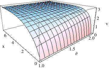
Refer to caption
Figure 2: The resulting value function.
Remark 6.1.

Figure 2 suggests that the value function is smooth and that therefore it should even be a classical solution of the HJB equation. However, proving smoothness is beyond the scope of this paper, since the HJB equation is degenerate elliptic on the whole domain, i.e., the diffusion coefficient is singular, which is highly non-standard.

Remark 6.2.

All of our examples give threshold strategies as the optimal dividend strategy. The convergence results from Fleming and Soner [10, Chapter IX] imply that, at least for our parameter sets, we can compute an ε\varepsilon-optimal value function corresponding to a threshold strategy.

7 Threshold strategies

The solution for the case where the drift θ\theta of the uncontrolled wealth process is deterministic as well as the numerical treatment of the Bayesian case suggest that the optimal dividend strategy is of threshold type, that is, there is a threshold level bb such that as soon as the wealth process exceeds the threshold level, dividends are paid at the maximum rate.

The numerical treatment for the Bayesian case further suggests that the threshold level depends on the estimate for θ\theta. In this section we formally define threshold strategies of this type and we give sufficient conditions under which they are admissible. We then proceed with giving a sufficient condition on a threshold strategy for being optimal. Of course one would also like to know whether there always exists at least one optimal strategy of threshold type. Unfortunately, this question has to remain open for the time being.

Definition 7.1.

Let b:[θ1,θ2]⟶[0,∞)b:[\theta_{1},\theta_{2}]\longrightarrow[0,\infty) be a continuous function and let b⁡(θ1)=b¯1b(\theta_{1})=\bar{b}_{1}, b⁡(θ2)=b¯2b(\theta_{2})=\bar{b}_{2}, where b¯1,b¯2\bar{b}_{1},\bar{b}_{2} are defined in (20).

A threshold strategy with threshold level bb is given by

utb=ub​(Xt,θt)={K,Xt≥b⁡(θt)0,Xt<b⁡(θt).u_{t}^{b}=u^{b}(X_{t},\theta_{t})=\begin{cases}K,&X_{t}\geq b(\theta_{t})\\ 0,&X_{t}<b(\theta_{t})\,.\end{cases}

First, we have to clarify whether threshold strategies are admissible. The system (8), (9), with uu replaced by a stationary Markov strategy, reads

Xt\displaystyle X_{t} =x+∫0t(θs−u⁡(Xs,θs))​𝑑s+σ​Wt,\displaystyle=x+\int_{0}^{t}(\theta_{s}-u(X_{s},\theta_{s}))\,ds+\sigma W_{t}\,, (24)
θt\displaystyle\theta_{t} =ϑ+1σ​∫0t(θs−θ1)​(θ2−θs)​d​Ws.\displaystyle=\vartheta+\frac{1}{\sigma}\int_{0}^{t}(\theta_{s}-\theta_{1})(\theta_{2}-\theta_{s})\,dW_{s}\,. (25)

A priori it is far from obvious that there exists a solution to the system (24), (25) if uu is a general measurable function. If uu is Lipschitz in both variables, then a solution exists by the classical theorem on existence and uniqueness of solutions of SDEs, see, e.g., [18, Chapter 2, Theorem 7]. But our threshold strategies do not fall in that category. In Leobacher et al. [19] it is shown that the system (8), (9) has a unique strong maximal local solution, if u=ubu=u^{b} is a threshold strategy with a threshold function b∈C5b\in C^{5}, satisfying

‖(1,−b′​(ϑ))⋅(σ1σ​(θ2−ϑ)​(ϑ−θ1))‖2≥c>0\displaystyle\left\|\left(1,-b^{\prime}(\vartheta)\right)\cdot\left(\begin{matrix}\sigma\\ \frac{1}{\sigma}(\theta_{2}-\vartheta)(\vartheta-\theta_{1})\end{matrix}\right)\right\|^{2}\geq c>0

for some constant c>0c>0. The latter condition means that the diffusion must not be parallel to the discontinuity of the drift. Since in our case b′b^{\prime} is a continuous function on a compact interval, this condition is equivalent to b′​(ϑ)≠σ2(θ2−ϑ)​(ϑ−θ1)b^{\prime}(\vartheta)\neq\frac{\sigma^{2}}{(\theta_{2}-\vartheta)(\vartheta-\theta_{1})}. Furthermore, as the diffusion coefficients are Lipschitz and the drift of XtX_{t} is bounded, we can apply [19, Theorem 3.3] and get that the system (24), (25) even has a unique strong global solution until the time τ\tau. Therefore, threshold strategies are indeed admissible if bb is sufficiently regular. In case of a threshold level like the one in Figure 1 where for small values of ϑ\vartheta we have b⁡(ϑ)=0b(\vartheta)=0, and then the curve grows monotonously, bb is clearly not sufficiently smooth. However, in that particular case that does not pose a problem, since bb equals zero at the point of the kink and the process is stopped once it reaches zero, i.e., when we have ruin. Thus we need not consider solutions starting in that point or passing through it.

The above discussion is summarized in the following definition and the subsequent lemma:

Definition 7.2.

Let u:[0,∞)×[θ1,θ2]⟶[0,K]u:[0,\infty)\times[\theta_{1},\theta_{2}]\longrightarrow[0,K] be a measurable function. We call uu an admissible Markov strategy if the system (24), (25) has a strong solution (Xt,θt)t≥0(X_{t},\theta_{t})_{t\geq 0} on [0,τ)[0,\tau), where, as before, τ=inf{t≥0:Xt≤0}\tau=\inf\{t\geq 0:X_{t}\leq 0\}. The set of admissible Markov strategies will be denoted by AMA_{M}.

Lemma 7.3.

Let b:[θ1,θ2]⟶[0,∞)b:[\theta_{1},\theta_{2}]\longrightarrow[0,\infty) be a function satisfying

  1. 1.

    bb is continuous;

  2. 2.

    b⁡(θ1)=b¯1b(\theta_{1})=\bar{b}_{1}, b⁡(θ2)=b¯2b(\theta_{2})=\bar{b}_{2};

  3. 3.

    on any interval on which b>0b>0 holds, bb is C5C^{5} and b′​(ϑ)≠σ2(θ2−ϑ)​(ϑ−θ1)b^{\prime}(\vartheta)\neq\frac{\sigma^{2}}{(\theta_{2}-\vartheta)(\vartheta-\theta_{1})}.

Then ub∈AMu^{b}\in A_{M}.

In the following we give a characterization of value functions corresponding to optimal threshold strategies.

Definition 7.4.

A function w:Ω¯→ℝw:\bar{\Omega}\rightarrow{\mathbb{R}} fulfills wx≤1w_{x}\leq 1 in the viscosity sense, if for all ψ∈C2​(Ω¯)\psi\in C^{2}(\bar{\Omega}) and for all (x¯,ϑ¯)∈Ω(\bar{x},\bar{\vartheta})\in\Omega such that (x¯,ϑ¯)(\bar{x},\bar{\vartheta}) is a minimum of w−ψw-\psi and w⁡(x¯,ϑ¯)=ψ⁡(x¯,ϑ¯)w(\bar{x},\bar{\vartheta})=\psi(\bar{x},\bar{\vartheta}), we have ψx​(x¯,ϑ¯)≤1\psi_{x}(\bar{x},\bar{\vartheta})\leq 1.

In other words, wx≤1w_{x}\leq 1 in the viscosity sense, if ww is a viscosity supersolution of ψx=1\psi_{x}=1.

Definition 7.5.

A function w:Ω¯→ℝw:\bar{\Omega}\rightarrow{\mathbb{R}} fulfills (wx​(x,ϑ)≤1⇔x≥b⁡(ϑ)w_{x}(x,\vartheta)\leq 1\Leftrightarrow x\geq b(\vartheta)) in the viscosity sense, if

ψx​(x¯,ϑ¯)≤1⇔x¯≥b⁡(ϑ¯)\psi_{x}(\bar{x},\bar{\vartheta})\leq 1\Leftrightarrow\bar{x}\geq b(\bar{\vartheta})

for all (x¯,ϑ¯)∈Ω(\bar{x},\bar{\vartheta})\in\Omega and for all ψ∈C2​(Ω¯)\psi\in C^{2}(\bar{\Omega}) such that (x¯,ϑ¯)(\bar{x},\bar{\vartheta}) is a minimum of w−ψw-\psi with w⁡(x¯,ϑ¯)=ψ⁡(x¯,ϑ¯)w(\bar{x},\bar{\vartheta})=\psi(\bar{x},\bar{\vartheta}).

Remark 7.6.
  1. 1.

    As for previous definitions of “viscosity sense” we have for w∈C1w\in C^{1} that [(wx​(x,ϑ)≤1⇔x≥b⁡(ϑ)w_{x}(x,\vartheta)\leq 1\Leftrightarrow x\geq b(\vartheta)) in the viscosity sense] ⇔\Leftrightarrow [(wx​(x,ϑ)≤1⇔x≥b⁡(ϑ)w_{x}(x,\vartheta)\leq 1\Leftrightarrow x\geq b(\vartheta)) ∀(x,ϑ)∈Ω\forall(x,\vartheta)\in\Omega].

  2. 2.

    Note that [ψx​(x,ϑ)≤1⇔x≥b⁡(ϑ)\psi_{x}(x,\vartheta)\leq 1\Leftrightarrow x\geq b(\vartheta) ∀(x,ϑ)∈Ω\forall(x,\vartheta)\in\Omega] ⇔\Leftrightarrow [(1−ψx​(x,ϑ))​(x−b⁡(ϑ))≥0(1-\psi_{x}(x,\vartheta))(x-b(\vartheta))\geq 0) ∀(x,ϑ)∈Ω\forall(x,\vartheta)\in\Omega].

In the following we denote the value function coming from a threshold strategy ub∈AMu^{b}\in A_{M} as J(b):=J(ub)J^{(b)}:=J^{(u^{b})} and
d​Xt:=(θt−utb)​d​t+σ​d​WtdX_{t}:=(\theta_{t}-u_{t}^{b})dt+\sigma dW_{t} , with X0=xX_{0}=x.
As in Asmussen and Taksar [2] one can not guarantee enough smoothness of J(b)J^{(b)} for an arbitrary threshold strategy. Therefore we characterize J(b)J^{(b)} as a viscosity solution of an appropriate PDE.

Lemma 7.7.

If the threshold strategy satisfies ub∈AMu^{b}\in A_{M}, and

J(b)​(x,ϑ)=𝔼x,ϑ​[∫0τe−δ​t​ub​(Xt,θt)​𝑑t]J^{(b)}(x,\vartheta)={\mathbb{E}}_{x,\vartheta}\left[\int_{0}^{\tau}e^{-\delta t}u^{b}(X_{t},\theta_{t})\,dt\right]

is continuous, J(b)J^{(b)} is a viscosity solution of

−δJ(b)+ℒJ(b)+K(1−Jx(b))1{x≥b(ϑ)}=0\displaystyle-\delta J^{(b)}+{\cal L}J^{(b)}+K(1-J_{x}^{(b)})1_{\{x\geq b(\vartheta)\}}=0 (26)

with the same boundary conditions as for VV in (12),(13),(14).

Proof.

Can be shown using standard techniques similar to the proof of Theorem 5.2. To show that J(b)J^{(b)} satisfies the boundary condition (14), i.e., J(b)J^{(b)} converges to the non-Bayesian solution for θ→θi\theta\rightarrow\theta_{i}, i=1,2i=1,2, we use the condition b⁡(θi)=bib(\theta_{i})=b_{i}. ∎

The following theorem provides the link between the value of a threshold strategy and the HJB equation (11).

Theorem 7.8.

Let a threshold level b:[θ1,θ2]⟶[0,∞)b:[\theta_{1},\theta_{2}]\longrightarrow[0,\infty) exist with ub∈AMu^{b}\in A_{M} and (Jx(b)​(x,ϑ)≤1⇔x≥b⁡(ϑ)J_{x}^{(b)}(x,\vartheta)\leq 1\Leftrightarrow x\geq b(\vartheta)) in the viscosity sense.

Then J(b)J^{(b)} is a viscosity solution of (11).

Proof.

First, we show that if J(b)J^{(b)} is a viscosity subsolution of (26), it is also a viscosity subsolution of (11).
Since J(b)J^{(b)} is a viscosity subsolution of (26), it holds that ∀ϕ∈C2​(Ω¯)\forall\phi\in C^{2}(\bar{\Omega}), ϕ≥J(b)\phi\geq J^{(b)} in Ω\Omega and for all (x¯,ϑ¯)(\bar{x},\bar{\vartheta}) where ϕ⁡(x¯,ϑ¯)=J(b)​(x¯,ϑ¯)\phi(\bar{x},\bar{\vartheta})=J^{(b)}(\bar{x},\bar{\vartheta}),

−δϕ+ℒϕ+K(1−ϕx)1{x¯≥b(ϑ¯)}≥0.-\delta\phi+{\cal L}\phi+K(1-\phi_{x})1_{\{\bar{x}\geq b(\bar{\vartheta})\}}\geq 0\,.

We have to show that

−δϕ+ℒϕ+K(1−ϕx)1{ϕx≤1}≥0-\delta\phi+{\cal L}\phi+K(1-\phi_{x})1_{\{\phi_{x}\leq 1\}}\geq 0

holds in the same points (x¯,ϑ¯)(\bar{x},\bar{\vartheta}). Therefore, it is enough to show that

−δϕ+ℒϕ+K(1−ϕx)1{x¯≥b(ϑ¯)}≤−δϕ+ℒϕ+K(1−ϕx)1{ϕx≤1},-\delta\phi+{\cal L}\phi+K(1-\phi_{x})1_{\{\bar{x}\geq b(\bar{\vartheta})\}}\leq-\delta\phi+{\cal L}\phi+K(1-\phi_{x})1_{\{\phi_{x}\leq 1\}}\,,

which is equivalent to

(1−ϕx)1{x¯≥b(ϑ¯)}≤(1−ϕx)1{ϕx≤1}.(1-\phi_{x})1_{\{\bar{x}\geq b(\bar{\vartheta})\}}\leq(1-\phi_{x})1_{\{\phi_{x}\leq 1\}}\,.

If ϕx≤1\phi_{x}\leq 1, we need that (1−ϕx)1{x¯≥b(ϑ¯)}≤(1−ϕx)(1-\phi_{x})1_{\{\bar{x}\geq b(\bar{\vartheta})\}}\leq(1-\phi_{x}), which is obviously true. If ϕx>1\phi_{x}>1, we need that (1−ϕx)1{x¯≥b(ϑ¯)}≤0(1-\phi_{x})1_{\{\bar{x}\geq b(\bar{\vartheta})\}}\leq 0. Since (1−ϕx)<0(1-\phi_{x})<0, this holds, too.
So J(b)J^{(b)} is a viscosity subsolution of (11).

It remains to show that if J(b)J^{(b)} is a viscosity supersolution of (26), it is also a viscosity supersolution of (11).
Since J(b)J^{(b)} is a viscosity supersolution of (26), it holds that ∀ψ∈C2​(Ω¯)\forall\psi\in C^{2}(\bar{\Omega}), ψ≤J(b)\psi\leq J^{(b)} in Ω\Omega and for all (x¯,ϑ¯)(\bar{x},\bar{\vartheta}) where ψ⁡(x¯,ϑ¯)=J(b)​(x¯,ϑ¯)\psi(\bar{x},\bar{\vartheta})=J^{(b)}(\bar{x},\bar{\vartheta}) it holds that

−δψ+ℒψ+K(1−ψx)1{x¯≥b(ϑ¯)}≤0.-\delta\psi+{\cal L}\psi+K(1-\psi_{x})1_{\{\bar{x}\geq b(\bar{\vartheta})\}}\leq 0\,.

We have to show that

−δψ+ℒψ+K(1−ψx)1{ϕx≤1}≤0-\delta\psi+{\cal L}\psi+K(1-\psi_{x})1_{\{\phi_{x}\leq 1\}}\leq 0

holds in the same points (x¯,ϑ¯)(\bar{x},\bar{\vartheta}). Hence, we need that

(1−ψx)1{x¯≥b(ϑ¯)}≥(1−ψx)1{ψx≤1}.(1-\psi_{x})1_{\{\bar{x}\geq b(\bar{\vartheta})\}}\geq(1-\psi_{x})1_{\{\psi_{x}\leq 1\}}\,.

If ψx<1\psi_{x}<1 or ψx>1\psi_{x}>1, we get (1−ψx)1{x¯≥b(ϑ¯)}≤(1−ψx)(1-\psi_{x})1_{\{\bar{x}\geq b(\bar{\vartheta})\}}\leq(1-\psi_{x}) and (1−ψx)1{x¯≥b(ϑ¯)}≤0(1-\psi_{x})1_{\{\bar{x}\geq b(\bar{\vartheta})\}}\leq 0, respectively. Therefore, we have to show that (1−ψx)1{x¯≥b(ϑ¯)}=(1−ψx)(1-\psi_{x})1_{\{\bar{x}\geq b(\bar{\vartheta})\}}=(1-\psi_{x}), if ψx<1\psi_{x}<1 and (1−ψx)1{x¯≥b(ϑ¯)}=0(1-\psi_{x})1_{\{\bar{x}\geq b(\bar{\vartheta})\}}=0, if ψx>1\psi_{x}>1. Hence, we need that ψx​(x¯,ϑ¯)≤1⇔x¯≥b⁡(ϑ¯)\psi_{x}(\bar{x},\bar{\vartheta})\leq 1\Leftrightarrow\bar{x}\geq b(\bar{\vartheta}).

From the statement of the theorem we have that (Jx(b)​(x,ϑ)≤1⇔x≥b⁡(ϑ)J_{x}^{(b)}(x,\vartheta)\leq 1\Leftrightarrow x\geq b(\vartheta)) in the viscosity sense, which is actually equivalent to what we need. Thus, J(b)J^{(b)} is a viscosity supersolution of (11).

Altogether, J(b)J^{(b)} is a viscosity solution of (11). ∎

Corollary 7.9.

Let J(b)J^{(b)} be like in Theorem 7.8. Then J(b)=VJ^{(b)}=V.

Proof.

Since VV is unique viscosity solution of (11) due to Theorem 5.3, J(b)=VJ^{(b)}=V. ∎

Altogether, we now know that if ub∈AMu^{b}\in A_{M} with a threshold level bb and corresponding value function J(b)J^{(b)} such that Jx(b)​(x,ϑ)≤1⇔x≥b⁡(ϑ)J^{(b)}_{x}(x,\vartheta)\leq 1\Leftrightarrow x\geq b(\vartheta) in the viscosity sense, then J(b)=VJ^{(b)}=V and ubu^{b} is the optimal control strategy.

8 Finite time ruin probabilities

In this section we will determine the finite time ruin probability of the uncontrolled process

pZ:=ℙz,ϑ​(τZ≤t),p^{Z}:={\mathbb{P}}_{z,\vartheta}(\tau^{Z}\leq t)\,,

where τZ:=inf{s≥0Zs≤0}\tau^{Z}:=\inf\{s\geq 0\,\vline\,Z_{s}\leq 0\}, for all t≥0t\geq 0. ℙz,ϑ{\mathbb{P}}_{z,\vartheta} abbreviates the probability given the initial values Z0=zZ_{0}=z and θ0=ϑ\theta_{0}=\vartheta.
Furthermore, we will consider the finite time ruin probability of our controlled process, assuming that the control variable follows a threshold strategy as defined in Section 7. So

d​Xt=θt​d​t+σ​d​Wt−d​Lt,dX_{t}=\theta_{t}\,dt+\sigma dW_{t}-dL_{t}\,,

where X0=x=zX_{0}=x=z, and Lt=∫0tusb​𝑑sL_{t}=\int_{0}^{t}u_{s}^{b}\,ds.
The finite time ruin probability is denoted as

pX:=ℙx,ϑ​(τ≤t).p^{X}:={\mathbb{P}}_{x,\vartheta}(\tau\leq t)\,.

Trivially, for z≤0z\leq 0, the finite time ruin probabilities pZp^{Z} and pXp^{X} are both equal to 1. Subsequently, we will tacitly assume that z>0z>0.

Remark 8.1.

For constant and observable θt=θ¯\theta_{t}=\bar{\theta} a classical application of Girsanov’s theorem and the reflection principle yields that the finite time ruin probability of the uncontrolled process ZZ is given by

pθ¯Z:=𝔼((1+e−2​θ¯σ2​Zt) 1{Zt≤0})=N(−θ¯​t+zσ​t)+e−2​θ¯​zσ2N(θ¯​t−zσ​t),p^{Z}_{\bar{\theta}}:={\mathbb{E}}\left(\left(1+e^{-\frac{2\bar{\theta}}{\sigma^{2}}Z_{t}}\right)\,1_{\{Z_{t}\leq 0\}}\right)=N\left(-\frac{\bar{\theta}t+z}{\sigma\sqrt{t}}\right)+e^{-\frac{2\bar{\theta}z}{\sigma^{2}}}N\left(\frac{\bar{\theta}t-z}{\sigma\sqrt{t}}\right)\,,

where NN is the cumulative distribution function of the standard normal distribution (cf. Karatzas and Shreve [16, p. 197]).

Now we want to calculate the finite time ruin probability for unobservable θ\theta. In Elliott et al. [9] results from filtering theory are applied to a general hidden Markov model and a PDE is derived, the solution of which is proven to be the finite time survival probability. We apply a different filter to overcome uncertainty, but after that, we use a similar result for our processes ZZ and XX. From the finite time survival probability we easily get the finite time ruin probability, which is just the complementary probability.
Let

ℒZ​(ρ⁡(z,ϑ))=ϑ​ρz+σ22​ρz​z+12​σ2​(ϑ−θ1)2​(θ2−ϑ)2​ρϑ​ϑ+(ϑ−θ1)​(θ2−ϑ)​ρz​ϑ{\cal L}^{Z}(\rho(z,\vartheta))=\vartheta\rho_{z}+\frac{\sigma^{2}}{2}\rho_{zz}+\frac{1}{2\sigma^{2}}(\vartheta-\theta_{1})^{2}(\theta_{2}-\vartheta)^{2}\rho_{\vartheta\vartheta}+(\vartheta-\theta_{1})(\theta_{2}-\vartheta)\rho_{z\vartheta}

be the infinitesimal generator of ZZ and let ℒZ,(0,∞)​(ρ⁡(z,ϑ)):=1(0,∞)​(z)​ℒZ​(ρ⁡(z,ϑ)){\cal L}^{Z,(0,\infty)}(\rho(z,\vartheta)):=1_{(0,\infty)}(z){\cal L}^{Z}(\rho(z,\vartheta)), where 1(0,∞)1_{(0,\infty)} is the indicator function of the domain (0,∞)(0,\infty).
Furthermore, let

ℒX​(ρ⁡(x,ϑ))=(ϑ−ub)​ρx+σ22​ρx​x+12​σ2​(ϑ−θ1)2​(θ2−ϑ)2​ρϑ​ϑ+(ϑ−θ1)​(θ2−ϑ)​ρx​ϑ{\cal L}^{X}(\rho(x,\vartheta))=(\vartheta-u^{b})\rho_{x}+\frac{\sigma^{2}}{2}\rho_{xx}+\frac{1}{2\sigma^{2}}(\vartheta-\theta_{1})^{2}(\theta_{2}-\vartheta)^{2}\rho_{\vartheta\vartheta}+(\vartheta-\theta_{1})(\theta_{2}-\vartheta)\rho_{x\vartheta}

be the infinitesimal generator of XX and let ℒX,(0,∞)​(ρ⁡(z,ϑ)):=1(0,∞)​(x)​ℒX​(ρ⁡(x,ϑ)){\cal L}^{X,(0,\infty)}(\rho(z,\vartheta)):=1_{(0,\infty)}(x){\cal L}^{X}(\rho(x,\vartheta)).
Then the following theorem, similar to Elliott et al. [9, Theorem 4.1], holds.

Theorem 8.2.
  1. 1.

    If ΦZ​(t,z,ϑ)\Phi^{Z}(t,z,\vartheta) is a smooth solution to

    ∂ΦZ∂t​(t,z,ϑ)=ℒZ,(0,∞)​(ΦZ​(t,z,ϑ))\displaystyle\frac{\partial\Phi^{Z}}{\partial t}(t,z,\vartheta)={\cal L}^{Z,(0,\infty)}\left(\Phi^{Z}(t,z,\vartheta)\right) (27)

    with initial condition

    ΦZ​(0,z,ϑ)=1(0,∞)​(z)\Phi^{Z}(0,z,\vartheta)=1_{(0,\infty)}(z)

    and boundary conditions

    ΦZ​(t,0,ϑ)\displaystyle\Phi^{Z}(t,0,\vartheta) =0,\displaystyle=0\,,
    ΦZ​(t,B,ϑ)\displaystyle\Phi^{Z}(t,B,\vartheta) =1​ for ​B→∞,\displaystyle=1\,\mbox{ for }B\rightarrow\infty\,,

    and ΦZ​(t,z,θi)\Phi^{Z}(t,z,\theta_{i}), i∈{θ1,θ2}i\in\{\theta_{1},\theta_{2}\} is the solution of the PDE for fixed ϑ=θi\vartheta=\theta_{i}, then

    ΦZ​(t,z,ϑ)=ℙz,ϑ​(τZ>t).\Phi^{Z}(t,z,\vartheta)={\mathbb{P}}_{z,\vartheta}(\tau^{Z}>t)\,.
  2. 2.

    If ΦX​(t,x,ϑ)\Phi^{X}(t,x,\vartheta) is a smooth solution to

    ∂ΦX∂t​(t,x,ϑ)=ℒX,(0,∞)​(ΦX​(t,x,ϑ))\displaystyle\frac{\partial\Phi^{X}}{\partial t}(t,x,\vartheta)={\cal L}^{X,(0,\infty)}\left(\Phi^{X}(t,x,\vartheta)\right) (28)

    with initial condition

    ΦX​(0,x,ϑ)=1(0,∞)​(x)\Phi^{X}(0,x,\vartheta)=1_{(0,\infty)}(x)

    and boundary conditions

    ΦX​(t,0,ϑ)\displaystyle\Phi^{X}(t,0,\vartheta) =0,\displaystyle=0\,,
    ΦX​(t,B,ϑ)\displaystyle\Phi^{X}(t,B,\vartheta) =1​ for ​B→∞,\displaystyle=1\,\mbox{ for }B\rightarrow\infty\,,

    and ΦX​(t,x,θi)\Phi^{X}(t,x,\theta_{i}), i∈{θ1,θ2}i\in\{\theta_{1},\theta_{2}\} is the solution of the PDE for fixed ϑ=θi\vartheta=\theta_{i}, then

    ΦX​(t,x,ϑ)=ℙx,ϑ​(τ>t).\Phi^{X}(t,x,\vartheta)={\mathbb{P}}_{x,\vartheta}(\tau>t)\,.
Proof.

Similar to the proof of Elliott et al. [9, Theorem 4.1]. ∎

Remark 8.3.

From the finite time survival probability we easily get the finite time ruin probability

pZ=1−ΦZ​(t,z,ϑ),\displaystyle p^{Z}=1-\Phi^{Z}(t,z,\vartheta)\,,
pX=1−ΦX​(t,x,ϑ).\displaystyle p^{X}=1-\Phi^{X}(t,x,\vartheta)\,.

We solved the PDEs numerically. Note that in our computations the boundary conditions for the ϑ\vartheta-variable are the numerical solutions of the corresponding PDEs for fixed ϑ=θ1\vartheta=\theta_{1} and ϑ=θ2\vartheta=\theta_{2}, respectively.

Figure 3 shows the finite time ruin probability in the uncontrolled and the controlled situation for the parameter choices σ=1\sigma=1, θ1=1\theta_{1}=1, t=10t=10, and θ2=2\theta_{2}=2, K=0.9K=0.9, B=4.17B=4.17, and θ2=4\theta_{2}=4, K=1.5K=1.5, B=7.46B=7.46. The boundary curve coincides with the deterministic situation, where θ=θi\theta=\theta_{i}, i=1,2i=1,2. One can see that, depending on the estimate of θ\theta, the difference between the controlled and the uncontrolled situation varies.

Refer to caption
Refer to caption
Refer to caption
Refer to caption
Refer to caption
Refer to caption
Figure 3: The finite time ruin probability pZp^{Z} (left), pXp^{X} (middle), and pX−pZp^{X}-p^{Z} (right).
Remark 8.4.

Note that for the uncontrolled process an alternative way to calculate pZp^{Z} is

pZ=q​pθ1Z+(1−q)​pθ2Z.\displaystyle p^{Z}=qp^{Z}_{\theta_{1}}+(1-q)p^{Z}_{\theta_{2}}\,.

9 Conclusion and open problems

We have presented a dividend optimization problem under partial information where the drift coefficient of the diffusion firm value process is a-priori unknown. We have shown how the drift coefficient can be estimated and we have derived the HJB equation for the stochastic optimal control problem.

It turns out that the optimal value function of the problem is the unique viscosity solution of the HJB equation, which allows for a numerical treatment of the problem. The numerical method gives an approximation to the optimal dividend policy and the corresponding value function. The treated examples suggest that threshold strategies are the optimal ones and we have discussed those strategies in more detail.

Finally, we have derived a PDE for the finite time ruin probability in our model and we have computed concrete examples numerically, both for the uncontrolled and controlled process.

As already mentioned in Section 7, a proof that there is always an optimal strategy of threshold type is yet to be found. The results of the numerical calculations suggest that this is the case. In addition, the plots of the corresponding value functions look smooth, so that one may have the hope that it is actually a classical solution to the HJB equation. Due to the degeneracy of the diffusion coefficient, a proof for this is beyond reach at the moment. We formulate the following conjectures:

Conjecture 1.

The optimal value function VV is C2C^{2} and is a classical solution to the HJB equation (11) with boundary conditions (12), (13), (14). Moreover, there always exists an admissible threshold strategy ubu^{b} such that V=J(b)V=J^{(b)}.

Conjecture 2.

Let b¯​(θ)\bar{b}(\theta) denote the optimal threshold for the non-Bayesian case and let bb be our optimal threshold function. From Figure 1 one would guess that

  1. 1.

    min⁡(b¯​(θ1),b¯​(θ2))≤b⁡(θ)≤max⁡(b¯​(θ1),b¯​(θ2))\min(\bar{b}(\theta_{1}),\bar{b}(\theta_{2}))\leq b(\theta)\leq\max(\bar{b}(\theta_{1}),\bar{b}(\theta_{2})); in particular, if b¯​(θ1)=b¯​(θ2)\bar{b}(\theta_{1})=\bar{b}(\theta_{2}) then bb does not depend on the Bayesian estimator;

  2. 2.

    if 0<b¯​(θ1)<b¯​(θ2)0<\bar{b}(\theta_{1})<\bar{b}(\theta_{2}), then bb is strictly increasing and strictly concave;

  3. 3.

    if b¯​(θ1)>b¯​(θ2)>0\bar{b}(\theta_{1})>\bar{b}(\theta_{2})>0, then bb is strictly decreasing and strictly convex.

Appendix A Supplementary proofs

Proof of Theorem 5.2.

We have to show that VV is both a viscosity sub- and supersolution.

VV is a viscosity supersolution: Let ψ∈C2​(Ω¯)\psi\in C^{2}(\bar{\Omega}), ψ≤V\psi\leq V and (x¯,ϑ¯)(\bar{x},\bar{\vartheta}) such that V⁡(x¯,ϑ¯)=ψ⁡(x¯,ϑ¯)V(\bar{x},\bar{\vartheta})=\psi(\bar{x},\bar{\vartheta}).
From the dynamic programming principle we have

ψ⁡(x¯,ϑ¯)=V⁡(x¯,ϑ¯)\displaystyle\psi(\bar{x},\bar{\vartheta})=V(\bar{x},\bar{\vartheta}) =supu∈[0,K]𝔼x¯,ϑ¯​(∫0τ∧ηe−δ​t​ut​𝑑t+e−δ⁡(τ∧η)​V​(Xτ∧η,θτ∧η))\displaystyle=\sup_{u\in[0,K]}{\mathbb{E}}_{\bar{x},\bar{\vartheta}}\left(\int_{0}^{\tau\wedge\eta}e^{-\delta t}u_{t}\,dt+e^{-\delta(\tau\wedge\eta)}V(X_{\tau\wedge\eta},\theta_{\tau\wedge\eta})\right)
≥𝔼x¯,ϑ¯​(u​1−e−δ⁡(τ∧η)δ+e−δ⁡(τ∧η)​ψ​(Xτ∧η,θτ∧η))\displaystyle\geq{\mathbb{E}}_{\bar{x},\bar{\vartheta}}\left(u\frac{1-e^{-\delta(\tau\wedge\eta)}}{\delta}+e^{-\delta(\tau\wedge\eta)}\psi(X_{\tau\wedge\eta},\theta_{\tau\wedge\eta})\right)

for any fixed u∈[0,K]u\in[0,K].
Applying Itô’s formula to ψ\psi, noting that the stochastic integrals are martingales, dividing by η\eta and letting η→0\eta\rightarrow 0 gives

0≥u−δ​ψ​(x¯,ϑ¯)+ℒ​ψ​(x¯,ϑ¯)−u​ψx​(x¯,ϑ¯).0\geq u-\delta\psi(\bar{x},\bar{\vartheta})+{\cal L}\psi(\bar{x},\bar{\vartheta})-u\,\psi_{x}(\bar{x},\bar{\vartheta})\,.

Since uu was arbitrary we get

0≥−δ​ψ​(x¯,ϑ¯)+ℒ​ψ​(x¯,ϑ¯)+supu∈[0,K](u⁡(1−ψx​(x¯,ϑ¯))).0\geq-\delta\psi(\bar{x},\bar{\vartheta})+{\cal L}\psi(\bar{x},\bar{\vartheta})+\sup_{u\in[0,K]}\left(u(1-\psi_{x}(\bar{x},\bar{\vartheta}))\right)\,.

So VV is a viscosity supersolution.

VV is a viscosity subsolution: For ε>0\varepsilon>0 let η>0\eta>0 with ε<η2\varepsilon<\eta^{2}.
Let uεu^{\varepsilon} be the density of an ε\varepsilon-optimal dividend policy, i.e., J(uε)≥V−ε,J^{(u^{\varepsilon})}\geq V-\varepsilon, and denote the firm value coming from uεu^{\varepsilon} as XεX^{\varepsilon}. Furthermore, let ϕ∈C2​(Ω¯)\phi\in C^{2}(\bar{\Omega}), ϕ≥V\phi\geq V and (x¯,ϑ¯)(\bar{x},\bar{\vartheta}) such that ϕ⁡(x¯,ϑ¯)=V⁡(x¯,ϑ¯)\phi(\bar{x},\bar{\vartheta})=V(\bar{x},\bar{\vartheta}).

ϕ⁡(x¯,ϑ¯)−ε\displaystyle\phi(\bar{x},\bar{\vartheta})-\varepsilon =V⁡(x¯,ϑ¯)−ε≤𝔼x¯,ϑ¯​(∫0τ∧ηe−δ​t​utε​𝑑t+e−δ⁡(τ∧η)​V​(Xτ∧ηε,θτ∧η))\displaystyle=V(\bar{x},\bar{\vartheta})-\varepsilon\leq{\mathbb{E}}_{\bar{x},\bar{\vartheta}}\left(\int_{0}^{\tau\wedge\eta}e^{-\delta t}u_{t}^{\varepsilon}\,dt+e^{-\delta(\tau\wedge\eta)}V(X_{\tau\wedge\eta}^{\varepsilon},\theta_{\tau\wedge\eta})\right)
≤𝔼x¯,ϑ¯​(∫0τ∧ηe−δ​t​utε​𝑑t+e−δ⁡(τ∧η)​ϕ​(Xτ∧ηε,θτ∧η))\displaystyle\leq{\mathbb{E}}_{\bar{x},\bar{\vartheta}}\left(\int_{0}^{\tau\wedge\eta}e^{-\delta t}u_{t}^{\varepsilon}dt+e^{-\delta(\tau\wedge\eta)}\phi(X_{\tau\wedge\eta}^{\varepsilon},\theta_{\tau\wedge\eta})\right)
=𝔼x¯,ϑ¯​(∫0τ∧ηe−δ​t​utε​𝑑t+e−δ⁡(τ∧η)​(ϕ⁡(x¯,ϑ¯)+∫0τ∧ηℒ​ϕ​𝑑t−∫0τ∧ηϕx​utε​𝑑t)),\displaystyle={\mathbb{E}}_{\bar{x},\bar{\vartheta}}\left(\int_{0}^{\tau\wedge\eta}e^{-\delta t}u_{t}^{\varepsilon}dt+e^{-\delta(\tau\wedge\eta)}\left(\phi(\bar{x},\bar{\vartheta})+\int_{0}^{\tau\wedge\eta}{\cal L}\phi\,dt-\int_{0}^{\tau\wedge\eta}\phi_{x}u_{t}^{\varepsilon}\,dt\right)\right)\,,

where we applied Itô’s formula and used that the stochastic integrals are martingales. Now, we divide by η\eta and let η→0\eta\rightarrow 0. Since ε<η2,ε→0\varepsilon<\eta^{2},\varepsilon\rightarrow 0 and εη→0\frac{\varepsilon}{\eta}\rightarrow 0. Thus,

(ℒ−δ)​ϕ+uε​(1−ϕx)≥0.({\cal L}-\delta)\phi+u^{\varepsilon}(1-\phi_{x})\geq 0\,.

Since uε​(1−ϕx)≤supu∈[0,K]u⁡(1−ϕx)u^{\varepsilon}(1-\phi_{x})\leq\sup_{u\in[0,K]}u(1-\phi_{x}), we get

(ℒ−δ)​ϕ+supu∈[0,K]u⁡(1−ϕx)≥0.({\cal L}-\delta)\phi+\sup_{u\in[0,K]}u(1-\phi_{x})\geq 0\,.

So V is also a viscosity subsolution.

In total VV is a viscosity solution of the HJB equation. ∎

Proof of Theorem 5.3.

We are going to prove the statement of the theorem by contradiction, using standard arguments from [5] and [22] adapted to our specific situation.
Suppose there exists (x0,ϑ0)∈Ω¯(x_{0},\vartheta_{0})\in\bar{\Omega} such that

w⁡(x0,ϑ0)−v⁡(x0,ϑ0)>0.\displaystyle w(x_{0},\vartheta_{0})-v(x_{0},\vartheta_{0})>0.

Since vv and ww are assumed to be bounded, we have

0<supΩ¯(w⁡(x,ϑ)−v⁡(x,ϑ))=:M<∞.\displaystyle 0<\sup_{\bar{\Omega}}(w(x,\vartheta)-v(x,\vartheta))=:M<\infty.

Now on ∂Ω¯\partial\bar{\Omega} we already have w≤vw\leq v by assumption, and lim supx→∞(w−v)​(x,ϑ)≤0\limsup_{x\rightarrow\infty}(w-v)(x,\vartheta)\leq 0 uniformly in ϑ\vartheta. Because of that and the continuity of ww and vv, we have that the maximum of w−vw-v needs to be attained at an interior point of Ω\Omega with finite xx-component. Therefore there exists B∈(0,∞)B\in(0,\infty) and (x¯,ϑ¯)∈(0,B)×(θ1,θ2)(\bar{x},\bar{\vartheta})\in(0,B)\times(\theta_{1},\theta_{2}), such that

M=w⁡(x¯,ϑ¯)−v⁡(x¯,ϑ¯).\displaystyle M=w(\bar{x},\bar{\vartheta})-v(\bar{x},\bar{\vartheta}).

Define for α>0\alpha>0,

Φα​(x,ϑ,y,ρ)=w⁡(x,ϑ)−v⁡(y,ρ)−12​α​((ϑ−ρ)2+(x−y)2),\displaystyle\Phi_{\alpha}(x,\vartheta,y,\rho)=w(x,\vartheta)-v(y,\rho)-\frac{1}{2\alpha}((\vartheta-\rho)^{2}+(x-y)^{2}),

for (x,ϑ,y,ρ)∈[0,B]×[θ1,θ2]×[0,B]×[θ1,θ2](x,\vartheta,y,\rho)\in[0,B]\times[\theta_{1},\theta_{2}]\times[0,B]\times[\theta_{1},\theta_{2}]. The function Φα\Phi_{\alpha} is again continuous and it attains a maximum on its compact domain at some point zα=(xα,ϑα,yα,ρα)z_{\alpha}=(x_{\alpha},\vartheta_{\alpha},y_{\alpha},\rho_{\alpha}). Furthermore we have

0<M\displaystyle 0<M =Φα​(x¯,ϑ¯,x¯,ϑ¯)≤Mα:=Φα​(zα)\displaystyle=\Phi_{\alpha}(\bar{x},\bar{\vartheta},\bar{x},\bar{\vartheta})\leq M_{\alpha}:=\Phi_{\alpha}(z_{\alpha})
≤w⁡(xα,ϑα)−v⁡(yα,ρα)≤M.\displaystyle\leq w(x_{\alpha},\vartheta_{\alpha})-v(y_{\alpha},\rho_{\alpha})\leq M.

The sequence {zα}α>0\{z_{\alpha}\}_{\alpha>0} on [0,B]×[θ1,θ2]×[0,B]×[θ1,θ2][0,B]\times[\theta_{1},\theta_{2}]\times[0,B]\times[\theta_{1},\theta_{2}] is bounded, therefore there exists a subsequence which converges to some value z~\tilde{z} when α→0\alpha\to 0. At the same time MαM_{\alpha} is bounded as well which implies that

12​α​((ϑα−ρα)2+(xα−yα)2)\displaystyle\frac{1}{2\alpha}((\vartheta_{\alpha}-\rho_{\alpha})^{2}+(x_{\alpha}-y_{\alpha})^{2})

is bounded as α→0\alpha\to 0. This implies that in the limit z~=(x~,ϑ~,x~,ϑ~)\tilde{z}=(\tilde{x},\tilde{\vartheta},\tilde{x},\tilde{\vartheta}), and directly from the inequality above we have x~=x¯\tilde{x}=\bar{x} and ϑ~=ϑ¯\tilde{\vartheta}=\bar{\vartheta}. In addition we obtain, at least along another subsequence Mα→MM_{\alpha}\to M and 12​α​((ϑα−ρα)2+(xα−yα)2)→0\frac{1}{2\alpha}((\vartheta_{\alpha}-\rho_{\alpha})^{2}+(x_{\alpha}-y_{\alpha})^{2})\to 0.
Without loss of generality we can assume that we already deal with the convergent subsequence and, since z¯\bar{z} is an interior point, that {zα}α>0∈(0,B)×(θ1,θ2)×(0,B)×(θ1,θ2)\{z_{\alpha}\}_{\alpha>0}\in(0,B)\times(\theta_{1},\theta_{2})\times(0,B)\times(\theta_{1},\theta_{2}).

In the following step we are going to apply Ishii’s Lemma in the form it is stated in [5, Theorem 3.2]. For this purpose we set

Fα​(x,ϑ,y,ρ)=12​α​((ϑ−ρ)2+(x−y)2),\displaystyle F^{\alpha}(x,\vartheta,y,\rho)=\frac{1}{2\alpha}((\vartheta-\rho)^{2}+(x-y)^{2}),

for (x,ϑ),(y,ρ)∈[0,B]×[θ1,θ2](x,\vartheta),(y,\rho)\in[0,B]\times[\theta_{1},\theta_{2}]. We have that w⁡(x,θ)−v⁡(y,ρ)−Fα​(x,θ,y,ρ)w(x,\theta)-v(y,\rho)-F^{\alpha}(x,\theta,y,\rho) attains a maximum in zα=(xα,ϑα,yα,ρα)z_{\alpha}=(x_{\alpha},\vartheta_{\alpha},y_{\alpha},\rho_{\alpha}). At these points we have

Dx,θ​Fα​(xα,ϑα,yα,ρα)=−Dy,ρ​Fα​(xα,ϑα,yα,ρα)=(xα−yααϑα−ραα),\displaystyle D_{x,\theta}F^{\alpha}(x_{\alpha},\vartheta_{\alpha},y_{\alpha},\rho_{\alpha})=-D_{y,\rho}F^{\alpha}(x_{\alpha},\vartheta_{\alpha},y_{\alpha},\rho_{\alpha})=\left(\begin{array}[]{c}\frac{x_{\alpha}-y_{\alpha}}{\alpha}\\ \frac{\vartheta_{\alpha}-\rho_{\alpha}}{\alpha}\end{array}\right),

and with I2I_{2} denoting the 2×22\times 2 identity matrix we can write

D2​Fα​(xα,ϑα,yα,ρα)=1α​(I2−I2−I2I2).\displaystyle D^{2}F^{\alpha}(x_{\alpha},\vartheta_{\alpha},y_{\alpha},\rho_{\alpha})=\frac{1}{\alpha}\left(\begin{array}[]{c c}I_{2}&-I_{2}\\ -I_{2}&I_{2}\end{array}\right).

From [5, Theorem 3.2] we obtain, for every ε>0\varepsilon>0, that there exist symmetric 2×22\times 2 matrices XX and YY such that (Dx,θ​Fα​(zα),X)∈J¯Ω¯2,+​w​(xα,ϑα)(D_{x,\theta}F^{\alpha}(z_{\alpha}),X)\in\bar{J}^{2,+}_{\bar{\Omega}}w(x_{\alpha},\vartheta_{\alpha}), which is the so-called superjet of ww at (xα,ϑα)(x_{\alpha},\vartheta_{\alpha}), and (−Dy,ρ​Fα​(zα),Y)∈J¯Ω¯2,−​v​(yα,ρα)(-D_{y,\rho}F^{\alpha}(z_{\alpha}),Y)\in\bar{J}^{2,-}_{\bar{\Omega}}v(y_{\alpha},\rho_{\alpha}), which is the so-called subjet of vv at (yα,ρα)(y_{\alpha},\rho_{\alpha}). In particular these matrices fulfill:

(X00−Y)≤1α​(I2−I2−I2I2)+εα2​(I2−I2−I2I2)2.\displaystyle\left(\begin{array}[]{c c}X&0\\ 0&-Y\end{array}\right)\leq\frac{1}{\alpha}\left(\begin{array}[]{c c}I_{2}&-I_{2}\\ -I_{2}&I_{2}\end{array}\right)+\frac{\varepsilon}{\alpha^{2}}\left(\begin{array}[]{c c}I_{2}&-I_{2}\\ -I_{2}&I_{2}\end{array}\right)^{2}.

Choosing ε=α\varepsilon=\alpha and taking the square of the matrix explicitly we get

(X00−Y)≤3α​(I2−I2−I2I2).\displaystyle\left(\begin{array}[]{c c}X&0\\ 0&-Y\end{array}\right)\leq\frac{3}{\alpha}\left(\begin{array}[]{c c}I_{2}&-I_{2}\\ -I_{2}&I_{2}\end{array}\right)\,.

Before using these super-subjet properties, we are going to derive a bound for the second order terms occurring in the HJB equation.
Define a​(x,ϑ)T=(σ,(ϑ−θ1)​(θ2−ϑ)σ)a(x,\vartheta)^{T}=(\sigma,\frac{(\vartheta-\theta_{1})(\theta_{2}-\vartheta)}{\sigma}) and write

X=(x11x12x12x22),Y=(y11y12y12y22),\displaystyle X=\left(\begin{array}[]{cc}x_{11}&x_{12}\\ x_{12}&x_{22}\end{array}\right)\,,\quad Y=\left(\begin{array}[]{cc}y_{11}&y_{12}\\ y_{12}&y_{22}\end{array}\right)\,,
Σ=(a⁡(xα,ϑα)​a​(xα,ϑα)Ta⁡(xα,ϑα)​a​(yα,ρα)Ta⁡(yα,ρα)​a​(xα,ϑα)Ta⁡(yα,ρα)​a​(yα,ρα)T).\displaystyle\Sigma=\left(\begin{array}[]{cc}a(x_{\alpha},\vartheta_{\alpha})a(x_{\alpha},\vartheta_{\alpha})^{T}&a(x_{\alpha},\vartheta_{\alpha})a(y_{\alpha},\rho_{\alpha})^{T}\\ a(y_{\alpha},\rho_{\alpha})a(x_{\alpha},\vartheta_{\alpha})^{T}&a(y_{\alpha},\rho_{\alpha})a(y_{\alpha},\rho_{\alpha})^{T}\end{array}\right)\,.

Now we are going to use inequality (A),

tr\displaystyle\mathrm{tr} [a⁡(xα,ϑα)​a​(xα,ϑα)T​X−a⁡(yα,ρα)​a​(yα,ρα)T​Y]\displaystyle[a(x_{\alpha},\vartheta_{\alpha})a(x_{\alpha},\vartheta_{\alpha})^{T}X-a(y_{\alpha},\rho_{\alpha})a(y_{\alpha},\rho_{\alpha})^{T}Y]
=\displaystyle= x11​σ2+2​x12​(ϑα−θ1)​(θ2−ϑα)+x22​(ϑα−θ1)2​(θ2−ϑα)2σ2\displaystyle x_{11}\sigma^{2}+2x_{12}(\vartheta_{\alpha}-\theta_{1})(\theta_{2}-\vartheta_{\alpha})+x_{22}\frac{(\vartheta_{\alpha}-\theta_{1})^{2}(\theta_{2}-\vartheta_{\alpha})^{2}}{\sigma^{2}}
−y11​σ2−2​y12​(ρα−θ1)​(θ2−ρα)−y22​(ρα−θ1)2​(θ2−ρα)2σ2\displaystyle-y_{11}\sigma^{2}-2y_{12}(\rho_{\alpha}-\theta_{1})(\theta_{2}-\rho_{\alpha})-y_{22}\frac{(\rho_{\alpha}-\theta_{1})^{2}(\theta_{2}-\rho_{\alpha})^{2}}{\sigma^{2}}
=\displaystyle= tr⁡[Σ⁡(X00−Y)]≤3α​tr​[Σ⁡(I2−I2−I2I2)]\displaystyle\mathrm{tr}\left[\Sigma\left(\begin{array}[]{c c}X&0\\ 0&-Y\end{array}\right)\right]\leq\frac{3}{\alpha}\mathrm{tr}\left[\Sigma\left(\begin{array}[]{c c}I_{2}&-I_{2}\\ -I_{2}&I_{2}\end{array}\right)\right]
=\displaystyle= 3α​tr​[(a⁡(xα,ϑα)−a⁡(yα,ρα))​(a⁡(xα,ϑα)−a⁡(yα,ρα))T]\displaystyle\frac{3}{\alpha}\mathrm{tr}[(a(x_{\alpha},\vartheta_{\alpha})-a(y_{\alpha},\rho_{\alpha}))(a(x_{\alpha},\vartheta_{\alpha})-a(y_{\alpha},\rho_{\alpha}))^{T}]
=\displaystyle= 3α​(ϑα−ρα)2​(ϑα−θ1−θ2+ρα)2σ2.\displaystyle\frac{3}{\alpha}(\vartheta_{\alpha}-\rho_{\alpha})^{2}\frac{(\vartheta_{\alpha}-\theta_{1}-\theta_{2}+\rho_{\alpha})^{2}}{\sigma^{2}}. (37)

The super-subjet notions appear in an equivalent formulation of the viscosity solution property based on second-order super and subdifferentials, see [10, Lemma 4.1, p. 211] or [5, Section 2].
Since ww is a viscosity subsolution of (11), the statement (Dx,θ​Fα​(zα),X)∈J¯Ω¯2,+​w​(xα,ϑα)(D_{x,\theta}F^{\alpha}(z_{\alpha}),X)\in\bar{J}^{2,+}_{\bar{\Omega}}w(x_{\alpha},\vartheta_{\alpha}) is equivalent to the existence of a subsolution test function at (xα,ϑα)(x_{\alpha},\vartheta_{\alpha}) with first derivative equal to Dx,θ​Fα​(zα)D_{x,\theta}F^{\alpha}(z_{\alpha}) and second derivative equal to XX. At the same time the statement (−Dy,ρ​Fα​(zα),Y)∈J¯Ω¯2,−​v​(yα,ρα)(-D_{y,\rho}F^{\alpha}(z_{\alpha}),Y)\in\bar{J}^{2,-}_{\bar{\Omega}}v(y_{\alpha},\rho_{\alpha}) is equivalent to the existence of a supersolution test function, again with the first derivative given by −Dy,ρ​Fα​(zα)-D_{y,\rho}F^{\alpha}(z_{\alpha}) and second derivative equal to YY.
Therefore, from the subsolution property of ww and the supersolution property of vv (using the above-mentioned derivatives for the respective test functions) we derive

−δ​w​(xα,ϑα)+ϑα​(xα−yα)α+12​tr​[a⁡(xα,ϑα)​a​(xα,ϑα)T​X]+supu∈[0,K]u⁡(1−(xα−yα)α)≥0,\displaystyle-\delta w(x_{\alpha},\vartheta_{\alpha})+\vartheta_{\alpha}\frac{(x_{\alpha}-y_{\alpha})}{\alpha}+\frac{1}{2}\mathrm{tr}[a(x_{\alpha},\vartheta_{\alpha})a(x_{\alpha},\vartheta_{\alpha})^{T}X]+\sup_{u\in[0,K]}u(1-\frac{(x_{\alpha}-y_{\alpha})}{\alpha})\geq 0\,,
−δ​v​(yα,ρα)+ρα​(xα−yα)α+12​tr​[a⁡(yα,ρα)​a​(yα,ρα)T​Y]+supu∈[0,K]u⁡(1−(xα−yα)α)≤0.\displaystyle-\delta v(y_{\alpha},\rho_{\alpha})+\rho_{\alpha}\frac{(x_{\alpha}-y_{\alpha})}{\alpha}+\frac{1}{2}\mathrm{tr}[a(y_{\alpha},\rho_{\alpha})a(y_{\alpha},\rho_{\alpha})^{T}Y]+\sup_{u\in[0,K]}u(1-\frac{(x_{\alpha}-y_{\alpha})}{\alpha})\leq 0.

Rearranging and using (37) yields

δ⁡(w⁡(xα,ϑα)−v⁡(yα,ρα))\displaystyle\delta(w(x_{\alpha},\vartheta_{\alpha})-v(y_{\alpha},\rho_{\alpha})) ≤(xα−yα)​(ϑα−ρα)α+12​tr​[Σ⁡(X00−Y)]\displaystyle\leq\frac{(x_{\alpha}-y_{\alpha})(\vartheta_{\alpha}-\rho_{\alpha})}{\alpha}+\frac{1}{2}\mathrm{tr}\left[\Sigma\left(\begin{array}[]{c c}X&0\\ 0&-Y\end{array}\right)\right]
≤(xα−yα)​(ϑα−ρα)α+32​α​(ϑα−ρα)2​(ϑα−θ1−θ2+ρα)2σ2\displaystyle\leq\frac{(x_{\alpha}-y_{\alpha})(\vartheta_{\alpha}-\rho_{\alpha})}{\alpha}+\frac{3}{2\alpha}(\vartheta_{\alpha}-\rho_{\alpha})^{2}\frac{(\vartheta_{\alpha}-\theta_{1}-\theta_{2}+\rho_{\alpha})^{2}}{\sigma^{2}}
≤max⁡{(xα−yα)2,(ϑα−ρα)2}α+32​α​(ϑα−ρα)2​(ϑα−θ1−θ2+ρα)2σ2.\displaystyle\leq\frac{\max\{(x_{\alpha}-y_{\alpha})^{2},(\vartheta_{\alpha}-\rho_{\alpha})^{2}\}}{\alpha}+\frac{3}{2\alpha}(\vartheta_{\alpha}-\rho_{\alpha})^{2}\frac{(\vartheta_{\alpha}-\theta_{1}-\theta_{2}+\rho_{\alpha})^{2}}{\sigma^{2}}.

In the above inequality the left-hand side converges to δ​M\delta M as α→0\alpha\to 0. Since Fα​(zα)→0F^{\alpha}(z_{\alpha})\to 0 at the same time (other terms are bounded), the right-hand side converges to 00, resulting in the contradiction δ​M≤0\delta M\leq 0, which concludes the proof of the theorem. ∎

Proof of Theorem 5.5.

Define φ⁡(x,ϑ):=1π​e−(x2+ϑ2)\varphi(x,\vartheta):=\frac{1}{\pi}e^{-(x^{2}+\vartheta^{2})} and let

φn​(x,ϑ):=n2​∫−∞∞∫−∞∞v⁡(x−s,ϑ−t)​φ​(n​s,n​t)​𝑑s​𝑑t.\varphi^{n}(x,\vartheta):=n^{2}\int_{-\infty}^{\infty}\int_{-\infty}^{\infty}v(x-s,\vartheta-t)\varphi(ns,nt)\,ds\,dt\,.

Note that as n→∞n\to\infty, φn→v\varphi^{n}\to v and ℒ​φn→ℒ​v{\cal L}\varphi^{n}\to{\cal L}v, see Wheeden and Zygmund [29].

Let u=(ut)t≥0u=(u_{t})_{t\geq 0} be an admissible strategy and let T∈ℕT\in{\mathbb{N}}. Then

e−δ⁡(T∧τ)​φn​(XT∧τ,θT∧τ)\displaystyle e^{-\delta(T\wedge\tau)}\varphi^{n}(X_{T\wedge\tau},\theta_{T\wedge\tau})
=\displaystyle= φn​(x,ϑ)+∫0T∧τe−δ​t​d​φn​(Xt,θt)+∫0T∧τφn​(Xt,θt)​d​(e−δ​t)\displaystyle\varphi^{n}(x,\vartheta)+\int_{0}^{T\wedge\tau}e^{-\delta t}\,d\varphi^{n}(X_{t},\theta_{t})+\int_{0}^{T\wedge\tau}\varphi^{n}(X_{t},\theta_{t})\,d(e^{-\delta t})
=\displaystyle= φn​(x,ϑ)+∫0T∧τe−δ​t​[−δ​φn​(Xt,θt)+ℒ​φn​(Xt,θt)−ut​φxn​(Xt,θt)]​𝑑t\displaystyle\varphi^{n}(x,\vartheta)+\int_{0}^{T\wedge\tau}e^{-\delta t}\left[-\delta\varphi^{n}(X_{t},\theta_{t})+{\cal L}\varphi^{n}(X_{t},\theta_{t})-u_{t}\varphi_{x}^{n}(X_{t},\theta_{t})\right]\,dt
+\displaystyle+ ∫0T∧τe−δ​t​[σ​φxn+(θt−θ1)​(θ2−θt)σ​φϑn]​d​Wt.\displaystyle\int_{0}^{T\wedge\tau}e^{-\delta t}\left[\sigma\varphi_{x}^{n}+\frac{(\theta_{t}-\theta_{1})(\theta_{2}-\theta_{t})}{\sigma}\varphi_{\vartheta}^{n}\right]\,dW_{t}\,.

After taking expectations, the stochastic integral vanishes. Therefore,

𝔼x,ϑ​(e−δ⁡(T∧τ)​φn​(XT∧τ,ϑT∧τ))\displaystyle{\mathbb{E}}_{x,\vartheta}\left(e^{-\delta(T\wedge\tau)}\varphi^{n}(X_{T\wedge\tau},\vartheta_{T\wedge\tau})\right)
=φn​(x,ϑ)+𝔼x,ϑ​(∫0T∧τe−δ​t​[−δ​φn​(Xt,θt)+ℒ​φn​(Xt,θt)−ut​φxn​(Xt,θt)]​𝑑t).\displaystyle=\varphi^{n}(x,\vartheta)+{\mathbb{E}}_{x,\vartheta}\left(\int_{0}^{T\wedge\tau}e^{-\delta t}\left[-\delta\varphi^{n}(X_{t},\theta_{t})+{\cal L}\varphi^{n}(X_{t},\theta_{t})-u_{t}\varphi_{x}^{n}(X_{t},\theta_{t})\right]\,dt\right)\,.

Let ε>0\varepsilon>0. Since vv fulfills

−δ​v+ℒ​v+(1−vx)​u≤0a.e.-\delta v+{\cal L}v+(1-v_{x})u\leq 0\quad\mbox{a.e.}

we can choose nn large enough such that

−δ​φn+ℒ​φn+(1−φxn)​u≤ε,-\delta\varphi^{n}+{\cal L}\varphi^{n}+(1-\varphi^{n}_{x})u\leq\varepsilon\,,

and hence

ℒ​φn≤δ​φn−(1−φxn)​u+ε.{\cal L}\varphi^{n}\leq\delta\varphi^{n}-(1-\varphi^{n}_{x})u+\varepsilon\,.

Therefore we get

𝔼x,ϑ​(e−δ⁡(T∧τ)​φn​(XT∧τ,θT∧τ))\displaystyle{\mathbb{E}}_{x,\vartheta}\left(e^{-\delta(T\wedge\tau)}\varphi^{n}(X_{T\wedge\tau},\theta_{T\wedge\tau})\right)
≤φn​(x,ϑ)+𝔼x,ϑ​(∫0T∧τe−δ​t​[−δ​φn​(Xt,θt)+δ​φn​(Xt,θt)−(1−φxn​(Xt,θt))​ut+ε−ut​φxn​(Xt,θt)]​𝑑t)\displaystyle\leq\varphi^{n}(x,\vartheta)+{\mathbb{E}}_{x,\vartheta}\left(\int_{0}^{T\wedge\tau}e^{-\delta t}\left[-\delta\varphi^{n}(X_{t},\theta_{t})+\delta\varphi^{n}(X_{t},\theta_{t})-(1-\varphi_{x}^{n}(X_{t},\theta_{t}))u_{t}+\varepsilon-u_{t}\varphi_{x}^{n}(X_{t},\theta_{t})\right]\,dt\right)
=φn​(x,ϑ)−𝔼x,ϑ​(∫0T∧τe−δ​t​ut​𝑑t+ε​∫0T∧τe−δ​t​𝑑t).\displaystyle=\varphi^{n}(x,\vartheta)-{\mathbb{E}}_{x,\vartheta}\left(\int_{0}^{T\wedge\tau}e^{-\delta t}u_{t}\,dt+\varepsilon\int_{0}^{T\wedge\tau}e^{-\delta t}\,dt\right)\,.

Letting n→∞n\rightarrow\infty, we get by dominated convergence

𝔼x,ϑ​(e−δ⁡(T∧τ)​v​(XT∧τ,θT∧τ))≤v⁡(x,ϑ)−𝔼x,ϑ​(∫0T∧τe−δ​t​ut​𝑑t+ε​∫0T∧τe−δ​t​𝑑t).\displaystyle{\mathbb{E}}_{x,\vartheta}\left(e^{-\delta(T\wedge\tau)}v(X_{T\wedge\tau},\theta_{T\wedge\tau})\right)\leq v(x,\vartheta)-{\mathbb{E}}_{x,\vartheta}\left(\int_{0}^{T\wedge\tau}e^{-\delta t}u_{t}\,dt+\varepsilon\int_{0}^{T\wedge\tau}e^{-\delta t}\,dt\right)\,.

As ε\varepsilon was arbitrary, we further get

𝔼x,ϑ​(e−δ⁡(T∧τ)​v​(XT∧τ,θT∧τ))≤v⁡(x,ϑ)−𝔼x,ϑ​(∫0T∧τe−δ​t​ut​𝑑t),{\mathbb{E}}_{x,\vartheta}\left(e^{-\delta(T\wedge\tau)}v(X_{T\wedge\tau},\theta_{T\wedge\tau})\right)\leq v(x,\vartheta)-{\mathbb{E}}_{x,\vartheta}\left(\int_{0}^{T\wedge\tau}e^{-\delta t}u_{t}\,dt\right)\,,

and hence

𝔼x,ϑ​(e−δ⁡(T∧τ)​v​(XT∧τ,θT∧τ))+𝔼x,ϑ​(∫0T∧τe−δ​t​ut​𝑑t)≤v⁡(x,ϑ).{\mathbb{E}}_{x,\vartheta}\left(e^{-\delta(T\wedge\tau)}v(X_{T\wedge\tau},\theta_{T\wedge\tau})\right)+{\mathbb{E}}_{x,\vartheta}\left(\int_{0}^{T\wedge\tau}e^{-\delta t}u_{t}\,dt\right)\leq v(x,\vartheta)\,.

From the supersolution property we have that 𝔼x,ϑ​(e−δ⁡(T∧τ)​v​(XT∧τ,θT∧τ))≥0{\mathbb{E}}_{x,\vartheta}\left(e^{-\delta(T\wedge\tau)}v(X_{T\wedge\tau},\theta_{T\wedge\tau})\right)\geq 0. Thus we have, by Fatou’s Lemma,

J(u)​(x,ϑ)=𝔼x,ϑ​(∫0τe−δ​t​ut​𝑑t)≤lim infT→∞𝔼x,ϑ​(∫0τ∧Te−δ​t​ut​𝑑t)≤v⁡(x,ϑ).J^{(u)}(x,\vartheta)={\mathbb{E}}_{x,\vartheta}\left(\int_{0}^{\tau}e^{-\delta t}u_{t}\,dt\right)\leq\liminf_{T\rightarrow\infty}{\mathbb{E}}_{x,\vartheta}\left(\int_{0}^{\tau\wedge T}e^{-\delta t}u_{t}\,dt\right)\leq v(x,\vartheta)\,.

So for each control uu, vv dominates the value function. Taking the supremum over u∈[0,K]u\in[0,K] in the derivation, we get equality in the HJB equation and therefore

V⁡(x,ϑ)≤v⁡(x,ϑ),V(x,\vartheta)\leq v(x,\vartheta)\,,

which completes the proof. ∎

References

  • [1] H. Albrecher and S. Thonhauser. Optimality Results for Dividend Problems in Insurance. RACSAM Revista de la Real Academia de Ciencias Exactas, Fisicas y Naturales. Serie A. Matematicas, 103(2):295–320, 2009.
  • [2] S. Asmussen and M. Taksar. Controlled Diffusion Models for Optimal Dividend Pay-Out. Insurance: Mathematics and Economics, 20(1):1–15, 1997.
  • [3] B. Avanzi. Strategies for Dividend Distribution: A Review. North American Actuarial Journal, 13(2):217–251, 2009.
  • [4] P. Azcue and N. Muler. Optimal Reinsurance and Dividend Distribution Policies in the Cramér-Lundberg Model. Mathematical Finance, 25(2):261–308, 2005.
  • [5] M. Crandall, H. Ishii, and P. Lions. User’s Guide to Viscosity Solutions of Second Order Partial Differential Equations. Bulletin of the American Mathematical Society, 27(1):1–67, 1992.
  • [6] B. de Finetti. Su un’impostazione alternativa della teoria collettiva del rischio. Transactions of the XVth International Congress of Actuaries, 2:433–443, 1957.
  • [7] J.-P. Décamps and S. Villeneuve. Optimal dividend policy and growth option. Finance Stoch., 11(1):3–27, 2007.
  • [8] J.-P. Décamps and S. Villeneuve. A Bayesian Adaptive Singular Control Problem Arising from Corporate Finance, 2012. Slides of a talk given at Swissquote Conference on Liquidity and Systemic Risk, November, EPFL, Lausanne, Switzerland.
  • [9] R. Elliott, T. Siu, and H. Yang. Ruin Theory in a Hidden Markov-Modulated Risk Model. Stochastic Models, 27(3):474–489, 2011.
  • [10] W. Fleming and H. Soner. Controlled Markov Processes and Viscosity Solutions. Stochastic Modelling and Applied Probability. Springer, second edition, 2006.
  • [11] H. Gerber. On Optimal Cancellation of Policies. ASTIN Bulletin, 9(1):125–138, 1977.
  • [12] P. Grandits, F. Hubalek, W. Schachermayer, and M. Žigo. Optimal Expected Exponential Utility of Dividend Payments in a Brownian Risk Model. Scandinavian Actuarial Journal, 2:73–107, 2007.
  • [13] F. Hubalek and W. Schachermayer. Optimizing Expected Utility of Dividend Payments for a Brownian Risk Process and a Peculiar Nonlinear ODE. Insurance Math. Econom., 34(2):193–225, 2004.
  • [14] M. Jeanblanc-Piqué and A.N. Shiryaev. Optimization of the Flow of Dividends. Russian Math. Surveys, 50(2):257–277, 1995.
  • [15] Z. Jiang and M. Pistorius. Optimal Dividend Distribution under Markov Regime Switching. Finance and Stochastics, 16(3):449–476, 2012.
  • [16] I. Karatzas and S.E. Shreve. Brownian Motion and Stochastic Calculus. Graduate Texts in Mathematics. Springer-Verlag, New York, second edition, 1991.
  • [17] I. Karatzas and X. Zhao. Bayesian Adaptive Portfolio Optimization. In Options Pricing, Interest Rates and Risk Management. Cambridge University Press, 2001.
  • [18] N.V. Krylov. Controlled Diffusion Processes. Applications of Mathematics. Springer, 1980.
  • [19] G. Leobacher, M. Szölgyenyi, and S. Thonhauser. On the Existence of Solutions of a Class of SDEs with Discontinuous Drift and Singular Diffusion. 2013. Submitted, arXiv:1311.6226.
  • [20] R.S. Liptser and A.N. Shiryaev. Statistics of Random Processes I - General Theory. Applications of Mathematics. Springer, 1977.
  • [21] R.S. Liptser and A.N. Shiryaev. Statistics of Random Processes II - Applications. Applications of Mathematics. Springer, second edition, 2000.
  • [22] H. Pham. Continuous-Time Stochastic Control and Optimization with Financial Applications. Stochastic Modeling and Applied Probability. Springer, 2009.
  • [23] R. Radner and L. Shepp. Risk vs. Profit Potential: A Model for Corporate Strategy. Journal of Economic Dynamics and Control, 20(8):1373–1393, 1996.
  • [24] U. Rieder and N. Bäuerle. Portfolio Optimization with Unobservable Markov-Modulated Drift Processes. Journal of Applied Probability, 42:362–378, 2005.
  • [25] J. Sass and U. Haussmann. Optimizing the Terminal Wealth under Partial Information: the Drift Process as a Continuous Time Markov Chain. Finance and Stochastics, 8:553–577, 2004.
  • [26] H. Schmidli. Stochastic Control in Insurance. Probability and its Applications. Springer, 2008.
  • [27] S.E. Shreve, J.P. Lehoczky, and D.P. Gaver. Optimal Consumption for General Diffusions with Absorbing and Reflecting Barriers. SIAM Journal on Control and Optimization, 22(1):55–75, 1984.
  • [28] L. Sotomayor and A. Cadenillas. Classical and Singular Stochastic Control for the Optimal Dividend Policy when there is Regime Switching. Insurance: Mathematics and Economics, 48:344–354, 2011.
  • [29] R. Wheeden and A. Zygmund. Measure and Integral: An Introduction to Real Analysis. Pure and Applied Mathematics. Marcel Dekker Inc., 1977.