Extending the Nested Parallel Model to the Nested Dataflow Model with Provably Efficient Schedulers

A parallel algorithm can be represented by a directed acyclic graph (DAG) that contains only data dependencies, but not the control dependencies induced by the programming model. We call this the algorithm DAG. In an algorithm DAG, each vertex represents a piece of computation without any parallel constructs and each directed edge represents a data dependency from its source to the sink vertex. For example, Figure 1a is the algorithm DAG of the dynamic programming algorithm for the Longest Common Subsequence (LCS) problem. This DAG is a 2D array of vertices labeled $X(i,j)$, where the values with coordinates $i=0$ or $j=0$ are given. For all $i,j>0$, vertex $X(i,j)$ depends on vertices $X(i-1,j-1),X(i,j-1)$ and $X(i-1,j)$. In an algorithm DAG, there are two possible relations between any pair of vertices $x$ and $y$. If there is a path from $x$ to $y$ or from $y$ to $x$, one of them must be executed before the other, i.e. they have to be serialized; otherwise, the two vertices can run concurrently.

It is often tedious to specify the algorithm DAG by listing individual vertices and edges, and in many cases the DAG is not fully known until the computation has finished. Therefore, higher level programming models are used to provide a description of a possibly dynamic DAG. One such model is the nested parallel programming model (also known as fork-join model) in which DAGs can be constructed through recursive compositions based on two constructs, “$\mathrel{\hskip 1.0pt\|\hskip 1.0pt}$” (“parallel”) and “$\mathrel{\hskip 1.0pt;\hskip 1.0pt}$” (“serial”). In the nested parallel (NP) model, an algorithm DAG can be specified by a spawn tree, which is a recursive composition based on these two constructs. The internal nodes of the spawn tree are serial and parallel composition constructs while the leaves are strands — segments of serial code that contain no function calls, returns, or spawn operations. In a spawn tree, $a\mathrel{\hskip 1.0pt;\hskip 1.0pt}b$ is an infix shorthand for a node with $\mathrel{\hskip 1.0pt;\hskip 1.0pt}$ operator and $a$ and $b$ as left and right children and indicates that $b$ has a dependence on $a$ and thus cannot start until $a$ finishes, while $a\mathrel{\hskip 1.0pt\|\hskip 1.0pt}b$ indicates that $a$ and $b$ can run concurrently.

To express the LCS algorithm in the NP model, one might decompose the 2D array of vertices in the algorithm DAG into four smaller blocks, recursively solve the smaller instances of the LCS algorithms on these blocks, and compose them to by specifying the dependencies between them using $\mathrel{\hskip 1.0pt;\hskip 1.0pt}$ or $\mathrel{\hskip 1.0pt\|\hskip 1.0pt}$ constructs. Figure 1 illustrates the resulting spawn tree up to two levels of recursion. The NP model demands a serial composition between two subtrees of the spawn tree even if there is partial dependency between them: that is, a subset of vertices in the DAG corresponding to one of the subtrees depends on a subset of vertices corresponding to the other. As a result, while the spawn tree in the NP programming model can accurately retain the data dependencies of the algorithm DAG, it also introduces many artificial dependencies that are not necessary to maintain algorithm correctness. Artificial dependencies induced by the NP programming model between subtrees of the spawn tree in Figure 1 are shown overlaid by dashed arrows onto the algorithm DAG in Figure 1b. Many parallel algorithms, including dynamic programming algorithms and direct numerical algorithms, have artificial dependencies when expressed in the NP programming model than increase the span of the algorithm (e.g. the span of LCS in the NP model is $O(n\log n)$ as opposed to $O(n)$ of its algorithm DAG). The insufficiency of the nested parallel programming model in expressing partial dependencies in a spawn tree is the fundamental reason that causes artificial dependencies between subtrees of the spawn tree. This deficiency not only limits the parallelism of the algorithms exposed to schedulers, but also makes it difficult to simultaneously optimize for multiple complexity measures of the program, such as span and cache complexity [50]; previous empirical studies on scheduling NP programs have shown that this deficiency can inhibit effective load balance [48].

The nested dataflow model extends the NP model by introducing an additional composition construct, “$\mathrel{\hskip 1.0pt\leadsto\hskip 1.0pt}$”, which generalizes the existing “$\mathrel{\hskip 1.0pt\|\hskip 1.0pt}$” and “$\mathrel{\hskip 1.0pt;\hskip 1.0pt}$” constructs. Programs in both the NP and ND models are expressed as spawn trees, where the internal nodes are the composition constructs and the leaf nodes are strands. We refer to subtrees of the spawn tree as tasks or function calls. We refer to the subtree rooted at the $i$-th child of an internal node as its $i$-th subtask. In both the models, larger tasks can be defined by composing smaller tasks with the “$\mathrel{\hskip 1.0pt;\hskip 1.0pt}$” and “$\mathrel{\hskip 1.0pt\|\hskip 1.0pt}$” constructs. The ND model allows tasks to be defined as a composition using the additional binary construct, “$\mathrel{\hskip 1.0pt\leadsto\hskip 1.0pt}$”, which enables the specification of “partial dependencies” between subtasks. This represents an arbitrary middle-point between the “$\mathrel{\hskip 1.0pt;\hskip 1.0pt}$” construct (full dependency) and the “$\mathrel{\hskip 1.0pt\|\hskip 1.0pt}$” construct (zero dependency).

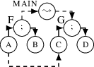
For example, consider the program represented by the spawn tree in Figure 5. The entire program, main, is comprised of two tasks F and G. Task F is the serial composition of tasks a and c, and task G is the serial composition of b and d. Task C depends on A, which creates a partial dependency from F to G. Instead of using a “$\mathrel{\hskip 1.0pt;\hskip 1.0pt}$” construct, which would block d until the completion of F (including both a and b), we denote the partial dependency with the “$\mathrel{\hskip 1.0pt\leadsto\hskip 1.0pt}$” construct in Figure 5.

We express this program as code in Figure 3. The partial dependency from F to G is specified with the rule $\stackrel{{\scriptstyle\textnormal{F}\textnormal{G}}}{{\mathrel{\hskip 1.0pt\leadsto\hskip 1.0pt}}}$. In order to specify that the only dependence is from a, the first subtask of F, to c, the first subtask of G, we write

The circled values denote relative pedigree, or pedigree in short, which represents the position of a nested function call in a spawn tree with respect to its ancestor [40]. We use wildcards \raisebox{-.9pt} {+}⃝ and \raisebox{-.9pt} {-}⃝ to represent the source and sink of the partial dependency. We then specify a set of fire rules to describe the partial dependence pattern of the “$\mathrel{\hskip 1.0pt\leadsto\hskip 1.0pt}$” construct between the source and the sink nodes. In the above case, we used \raisebox{-.9pt} {+}⃝\raisebox{-.9pt} {1}⃝ to denote the first subtask of the source, \raisebox{-.9pt} {+}⃝; similarly, \raisebox{-.9pt} {-}⃝\raisebox{-.9pt} {1}⃝ denotes the first subtask of the sink. The semicolon indicates a full dependency between them. In the context of main in Figure 3, \raisebox{-.9pt} {+}⃝ is bound to F and \raisebox{-.9pt} {-}⃝ to G, implying that there is a full dependency from \raisebox{-.9pt} {F}⃝\raisebox{-.9pt} {1}⃝, which refers to a, to \raisebox{-.9pt} {G}⃝\raisebox{-.9pt} {1}⃝, which refers to c. In the general case, we allow multiple rewriting rules in the definition of a fire construct, and “multilevel” pedigrees (e.g. \raisebox{-.9pt} {+}⃝\raisebox{-.9pt} {2}⃝\raisebox{-.9pt} {1}⃝ denotes the second subtask of the first subtask of the source) in each rule.

In the previous example, the dependency from a to c is a full dependency; that is, the entirety of a must be completed before c can start. However, this dependency itself may be artificial. Therefore, we allow the “$\mathrel{\hskip 1.0pt\leadsto\hskip 1.0pt}$” construct to be recursively defined using fire rules that themselves represent partial dependencies.

Consider the following divide-and-conquer algorithm for computing the matrix product $C+=A\times B$, which we denote $\textnormal{MM}(A,B,C)$. Let $C_{00},C_{01},C_{10}$ and $C_{11}$ denote the top left, bottom left, top right, and the bottom right quadrants of $C$ respectively. In the ND model, we can define $\textnormal{MM}(A,B,C)$ to be

Each quadrant of $C$ is written to by two of the eight subtasks; each such pair of subtasks must be serialized to avoid a data race. For this, we might naively define the fire construct “$\stackrel{{\scriptstyle MM}}{{\mathrel{\hskip 1.0pt\leadsto\hskip 1.0pt}}}$” between the immediate subtasks of $\textnormal{MM}(A,B,C)$ with a pair of fire rules:

However, notice that the dependency between first subtasks (as well as second subtasks), which is expressed with “$\mathrel{\hskip 1.0pt;\hskip 1.0pt}$” in the code above, is in reality a partial dependency. Furthermore, each of these partial dependencies has the same pattern as “$\stackrel{{\scriptstyle MM}}{{\mathrel{\hskip 1.0pt\leadsto\hskip 1.0pt}}}$”. Since this pattern repeats recursively down an arbitrary number of levels, the “$\stackrel{{\scriptstyle MM}}{{\mathrel{\hskip 1.0pt\leadsto\hskip 1.0pt}}}$” construct should have been described by the fire rules:

wherein “$\mathrel{\hskip 1.0pt;\hskip 1.0pt}$” is replaced by “$\stackrel{{\scriptstyle MM}}{{\mathrel{\hskip 1.0pt\leadsto\hskip 1.0pt}}}$”.

If the recursion terminates at the level indicated in Figure 5, the four instances of “$\stackrel{{\scriptstyle MM}}{{\mathrel{\hskip 1.0pt\leadsto\hskip 1.0pt}}}$” between leaves of the spawn tree will be interpreted as four full dependencies between the corresponding strands. If the recursion continues, the fire rules are used to further refine the dependencies. Whereas this algorithm has only one set of dependence patterns (fire rules), we will see algorithms with multiple types of fire rules in the next section.

The DRS iteratively constructs the dataflow edges, and equivalently the algorithm DAG, by starting with a single vertex representing the root of the spawn tree and successively applying DAG rewriting rules. Given a DAG $G$, a rewriting rule replaces a sub-graph that is isomorphic to $L$ with a copy of sub-graph $R=\langle V,E\rangle$, resulting in a new DAG $G^{\prime}$. There are two rewriting rules:

1. 1.

   Spawn Rule: A spawn rule corresponds to a spawn operation. Any current leaf of the spawn tree corresponds to a single-vertex no-edge subgraph $L=\langle\{\textnormal{a}\},\emptyset\rangle$ of the DAG. If it spawns, we rewrite the leaf as a (sub)tree rooted by either a “$\mathrel{\hskip 1.0pt;\hskip 1.0pt}$”, “$\mathrel{\hskip 1.0pt\|\hskip 1.0pt}$” or “$\mathrel{\hskip 1.0pt\leadsto\hskip 1.0pt}$’’ in the spawn tree.¹¹ 1 A leaf with a non-constant degree parallel construct such as a parallel for loop of tasks must be rewritten as an binary tree in our programming model. The root of the newly spawned (sub)tree inherits all incoming and outgoing dataflow arrows of the old leaf. For instance, if task a spawns b and c in serial, we rewrite the single-vertex, no-edge DAG $L$ to $R=\langle\{\textnormal{b},$“$\mathrel{\hskip 1.0pt;\hskip 1.0pt}$”$,\textnormal{c}\},\overrightarrow{\textnormal{b}\textnormal{c}}\rangle$, where $\overrightarrow{\textnormal{b}\textnormal{c}}$ is a solid dataflow arrow (directed edge) from b to c ($\overrightarrow{\textnormal{b}\textnormal{c}}$ is actually a shorthand for all-to-all dataflow arrows from all possible descendants of b to those of c, i.e. $\textnormal{b}\times\textnormal{c}$). If task a calls b and c in parallel, we rewrite it as $R=\langle\{\textnormal{b},$“$\mathrel{\hskip 1.0pt\|\hskip 1.0pt}$”$,\textnormal{c}\},\emptyset\rangle$. While the parallel construct introduces no dataflow arrows between b and c, a rewriting rule from its closest ancestor that is a “$\mathrel{\hskip 1.0pt\leadsto\hskip 1.0pt}$” construct can introduce dataflow arrows to these two nodes according to the fire rule. The semantics of non-binary serial and parallel constructs are similar. If task a invokes “$\textnormal{b}\mathrel{\hskip 1.0pt\leadsto\hskip 1.0pt}\textnormal{c}$”, we rewrite to $R=\langle\{\textnormal{b}\allowbreak,$“$\mathrel{\hskip 1.0pt\leadsto\hskip 1.0pt}$”$\allowbreak,\textnormal{c}\}\allowbreak,E^{\prime}\allowbreak\subseteq\allowbreak\textnormal{b}\allowbreak\times\allowbreak\textnormal{c}\allowbreak\rangle$, where $E^{\prime}$ is a dashed dataflow arrow and is the subset of all possible arrows from descendants of b to descendants of c to be defined by the fire rule as follows.

2. 2.

   Fire Rule: Given a dashed dataflow arrow between arbitrary source and sink nodes, including those from the left child of a fire construct to its right child, we (recursively) rewrite the arrow using the set of fire rules associated with it. These rules specify how the “$\mathrel{\hskip 1.0pt\leadsto\hskip 1.0pt}$” construct is rewritten to a set of dataflow arrows between the descendants of the source and the sink nodes, and their annotations. There are two possible cases for rewriting:

   • •

     If both operands a and b are strands, the dataflow arrow between them is rewritten as either “$\textnormal{a}\mathrel{\hskip 1.0pt;\hskip 1.0pt}\textnormal{b}$” or, if the fire construct has no rewriting rules, “$\textnormal{a}\mathrel{\hskip 1.0pt\|\hskip 1.0pt}\textnormal{b}$”.

   • •

     If the source task a of a “$\mathrel{\hskip 1.0pt\leadsto\hskip 1.0pt}$” construct is rewritten by a spawn rule into a tree containing $k$ subtasks, we add dataflow arrows $E^{\prime}\subseteq\{\textnormal{a}_{1},\dots\textnormal{a}_{k}\}\times\textnormal{b}$ to the resulting DAG, i.e. $R=\langle V,E\cup E^{\prime}\rangle$, where the arrows in $E^{\prime}$ and their labels is determined based on the fire rules of the “$\mathrel{\hskip 1.0pt\leadsto\hskip 1.0pt}$” construct as follows: for a fire rule of the form $\raisebox{0.5pt}{\textcircled{\raisebox{-.9pt} {+}}\textcircled{\raisebox{-.9pt} {i}}}p\stackrel{{\scriptstyle T}}{{\mathrel{\hskip 1.0pt\leadsto\hskip 1.0pt}}}\raisebox{0.5pt}{\textcircled{\raisebox{-.9pt} {-}}}q$ (where $p$ and $q$ are some pedigrees) from a to b, we add a dataflow arrow $\raisebox{0.5pt}{\textcircled{\raisebox{-.9pt} {+}}}p\stackrel{{\scriptstyle T}}{{\mathrel{\hskip 1.0pt\leadsto\hskip 1.0pt}}}\raisebox{0.5pt}{\textcircled{\raisebox{-.9pt} {-}}}q$ from $\textnormal{a}_{i}$ to b. An analogous rule applies when the sink spawns.

From the DRS, it is evident that the binary “$\mathrel{\hskip 1.0pt;\hskip 1.0pt}$” and “$\mathrel{\hskip 1.0pt\|\hskip 1.0pt}$” constructs are special cases of the “$\mathrel{\hskip 1.0pt\leadsto\hskip 1.0pt}$” construct. Four fire rules that recursively refine between both pairs of subtasks of \raisebox{-.9pt} {+}⃝ and \raisebox{-.9pt} {-}⃝ define the $\mathrel{\hskip 1.0pt;\hskip 1.0pt}$ construct, and an empty set of rules defines “$\mathrel{\hskip 1.0pt\|\hskip 1.0pt}$”. It is also straightforward to replace higher-degree “$\mathrel{\hskip 1.0pt;\hskip 1.0pt}$” and “$\mathrel{\hskip 1.0pt\|\hskip 1.0pt}$” constructs using “$\mathrel{\hskip 1.0pt\leadsto\hskip 1.0pt}$” if one so chooses.

In this section and, we express several typical $2$-way divide-and-conquer classical linear algebra and dynamic programming algorithms in the ND model. These include Triangular System Solver, Cholesky factorization, LU factorization with partial pivoting, Floyd-Warshall algorithm for All-Pairs-Shortest-Paths, and LCS. Note that in going from the NP to the ND model in these algorithms, the cache complexity of the depth-first traversal will not change as we leave the divide-and-conquer spawn tree unchanged. At the same time, we demonstrate that the algorithms have improved parallelism in the ND model. We do this by proving that their span is smaller than in the NP model. We will develop more sophisticated metrics to quantify parallelism in the presence of caches in Section 4; it turns out those metrics demonstrate improved parallelism in the ND model as well.

Equation (2) recursively solves TRS on four equally sized sub-quadrants $X_{00}$, $X_{01}$, $X_{10}$, and $X_{11}$, as graphically depicted in Figure 7. It can be expressed in the NP model as shown in Equation (3), where $\textnormal{MMS}(A,B,C)$ represents a cache-oblivious matrix multiplication and subtraction (identical to the one presented in Section 2, except instead of computing $C+=AB$ it computes $C-=AB$) with span $O(n)$ and using $O(n^{2})$ space.²² 2 There is also an $8$-way divide-and-conquer cache-oblivious parallel algorithm of MMS that has an optimal span of $O(\log^{2}n)$ but uses $O(n^{3})$ space which can be used to trade off span for space complexity.

The span of the TRS algorithm, expressed in the NP model is given by the recurrence $T_{\infty,\textnormal{TRS}}(n)=2T_{\infty,\textnormal{TRS}}(n/2)+T_{\infty,\textnormal{SMM}}(n/2)$, which evaluates to $O(n\log n)$, and is not optimal; a straightforward right-looking algorithm has a span of $O(n)$.

In Equation (4), we replace the “$\mathrel{\hskip 1.0pt;\hskip 1.0pt}$” constructs from the original schedule with “$\mathrel{\hskip 1.0pt\leadsto\hskip 1.0pt}$” construct, in order to remove artificial dependencies. Because the two “$\mathrel{\hskip 1.0pt\leadsto\hskip 1.0pt}$” constructs join different types of tasks, they have distinct types, which we denote “$\stackrel{{\scriptstyle TM}}{{\mathrel{\hskip 1.0pt\leadsto\hskip 1.0pt}}}$” and “$\stackrel{{\scriptstyle 2TM2T}}{{\mathrel{\hskip 1.0pt\leadsto\hskip 1.0pt}}}$”. Note that there are algorithms, e.g. Cholesky factorization, where two types of subtasks, say trs and mms, have more than one kind of partial dependency pattern between them based on where they occur. Each type of fire construct has different set of fire rules; in order to determine what these rules are, we expand an additional level of recursion to examine finer-grained data dependencies.

Notice that the source task of $\stackrel{{\scriptstyle 2TM2T}}{{\mathrel{\hskip 1.0pt\leadsto\hskip 1.0pt}}}$ is $((X_{00}\mathrel{\hskip 1.0pt\leftarrow\hskip 1.0pt}\textnormal{TRS}(T_{00},B_{00})\stackrel{{\scriptstyle TM}}{{\mathrel{\hskip 1.0pt\leadsto\hskip 1.0pt}}}\textnormal{MMS}(T_{10},X_{00},B_{10}))\mathrel{\hskip 1.0pt\|\hskip 1.0pt}(X_{01}\mathrel{\hskip 1.0pt\leftarrow\hskip 1.0pt}\textnormal{TRS}(T_{00},B_{01})\stackrel{{\scriptstyle TM}}{{\mathrel{\hskip 1.0pt\leadsto\hskip 1.0pt}}}\textnormal{MMS}(T_{10},X_{01},B_{11})))$, and the its sink is $(X_{10}\mathrel{\hskip 1.0pt\leftarrow\hskip 1.0pt}\textnormal{TRS}(T_{11},B_{10})\mathrel{\hskip 1.0pt\|\hskip 1.0pt}X_{11}\mathrel{\hskip 1.0pt\leftarrow\hskip 1.0pt}\textnormal{TRS}(T_{11},B_{11}))$. Since the left subtask of the sink can start as soon as the matrix multiply updating $B_{10}$ (which is the right subtask of the left subtask of the sink) is completed, and the right subtask of the sink analogously depends on the matrix multiply updating $B_{11}$, the fire rule for $\stackrel{{\scriptstyle 2T2M}}{{\mathrel{\hskip 1.0pt\leadsto\hskip 1.0pt}}}$ is simply:

Both the fire constructs in the fire rules are of type “$\stackrel{{\scriptstyle MT}}{{\mathrel{\hskip 1.0pt\leadsto\hskip 1.0pt}}}$” since the dependency structure is identical: the matrix updated in the source MMS operation is used as a dependency in the second argument of the TRS operation.

In order to determine the set of fire rules for “$\stackrel{{\scriptstyle MT}}{{\mathrel{\hskip 1.0pt\leadsto\hskip 1.0pt}}}$”, we expand a pair of subtasks connected by the “$\stackrel{{\scriptstyle MT}}{{\mathrel{\hskip 1.0pt\leadsto\hskip 1.0pt}}}$” construct to an additional level of recursion. For instance, we will expand the task $\textnormal{MMS}(T_{10},X_{00},B_{10})$ in equation Equation (7), which (as the source) binds to \raisebox{-.9pt} {+}⃝ in $\stackrel{{\scriptstyle TM}}{{\mathrel{\hskip 1.0pt\leadsto\hskip 1.0pt}}}$, and $X_{00}\mathrel{\hskip 1.0pt\leftarrow\hskip 1.0pt}\textnormal{TRS}(T_{11},B_{10})$ in Equation (6), which binds to \raisebox{-.9pt} {-}⃝. In the following program, we use $A_{00,11}$ to denote the bottom right quadrant of the top left quadrant of $A$.

The dependence of the sink task, \raisebox{-.9pt} {-}⃝, on the source task, \raisebox{-.9pt} {+}⃝, in “$\stackrel{{\scriptstyle MT}}{{\mathrel{\hskip 1.0pt\leadsto\hskip 1.0pt}}}$” is a result of requiring the value of matrix $B_{10}$ to be updated by \raisebox{-.9pt} {+}⃝ before \raisebox{-.9pt} {-}⃝ can use it in a computation. At a more fine-grained level, we can examine which quadrant of $B_{10}$ each subtask of \raisebox{-.9pt} {-}⃝ requires (and which subtask of \raisebox{-.9pt} {+}⃝ computes that quadrant) in order to calculate the fine-grained dependencies. For instance, consider the subtask $X_{00,00}\mathrel{\hskip 1.0pt\leftarrow\hskip 1.0pt}\textnormal{TRS}(T_{11,00},B_{10,00})$, whose pedigree is \raisebox{-.9pt} {-}⃝\raisebox{-.9pt} {1}⃝\raisebox{-.9pt} {1}⃝\raisebox{-.9pt} {1}⃝, which requires $B_{10,00}$. This quadrant of $B_{10}$ is updated in $\textnormal{MMS}(T_{10,01},X_{00,10},B_{10,00})$ of the source, whose pedigree is \raisebox{-.9pt} {+}⃝\raisebox{-.9pt} {2}⃝\raisebox{-.9pt} {1}⃝\raisebox{-.9pt} {1}⃝. Furthermore, notice that the dependency from \raisebox{-.9pt} {+}⃝\raisebox{-.9pt} {2}⃝\raisebox{-.9pt} {1}⃝\raisebox{-.9pt} {1}⃝ to \raisebox{-.9pt} {-}⃝\raisebox{-.9pt} {1}⃝\raisebox{-.9pt} {1}⃝\raisebox{-.9pt} {1}⃝ takes the same form as the dependency from \raisebox{-.9pt} {+}⃝ to \raisebox{-.9pt} {-}⃝ itself: the matrix updated by the source is the second argument in the sink. Therefore, the fire rule for this particular dependency is $\raisebox{0.5pt}{\textcircled{\raisebox{-.9pt} {+}}\textcircled{\raisebox{-.9pt} {2}}\textcircled{\raisebox{-.9pt} {1}}\textcircled{\raisebox{-.9pt} {1}}}\stackrel{{\scriptstyle TM}}{{\mathrel{\hskip 1.0pt\leadsto\hskip 1.0pt}}}\raisebox{0.5pt}{\textcircled{\raisebox{-.9pt} {-}}\textcircled{\raisebox{-.9pt} {1}}\textcircled{\raisebox{-.9pt} {1}}\textcircled{\raisebox{-.9pt} {1}}}$. Similar reasoning gives the remaining fire rules:

We now argue that the span of TRS in the ND model is $O(n)$. The span of an algorithm is the length of the longest path in its DAG. The algorithm DAG defined by TRS expressed in the ND model forms a periodic structure, a cross section of which can be seen in Figure 8, where squares represent matrix multiplications and triangles represent smaller TRS tasks (there are no edges between separate cross sections). The length of the longest path in the DAG, shown in blue, is $O(n)$.

We now formally prove that the algorithm we constructed in the ND model achieves this span. Let $T_{\infty,\textnormal{TRS}}(n)$ denote the span of TRS on a matrix with input size $n\times n$, and let $T_{\infty,\textnormal{TRS}\ p}(n)$ denote the span of the subtask with pedigree $p$ descended from TRS with input size $n\times n$. Furthermore, let $T_{\infty,\stackrel{{\scriptstyle TM}}{{\mathrel{\hskip 1.0pt\leadsto\hskip 1.0pt}}}}(n)$ denote the critical path length of a TRS composed with a matrix multiply by a “$\stackrel{{\scriptstyle TM}}{{\mathrel{\hskip 1.0pt\leadsto\hskip 1.0pt}}}$” construct, where both tasks are directly descended from a TRS of size $n\times n$. Note that it involves two tasks, a TRS and MMS, of size $n/2\times n/2$ each.

Since replacing a fire construct with a serial construct can only increase the span, it suffices to show that a version of the problem with some fire constructs replaced with serial constructs has optimal span. In this analysis, we will replace the “$\stackrel{{\scriptstyle 2TM2T}}{{\mathrel{\hskip 1.0pt\leadsto\hskip 1.0pt}}}$” construct with a serial composition, giving the following upper bound on the span of TRS in the ND model:

Since the right subtask of TRS is merely the parallel composition of two TRS operations, each on a matrix of size $n/2\times n/2$, the second term on the right reduces to the max of their (identical) spans, which is

The left subtask consists of two pairs (connected by a parallel composition), each consisting of a TRS task and a MMS task, connected by “$\stackrel{{\scriptstyle TM}}{{\mathrel{\hskip 1.0pt\leadsto\hskip 1.0pt}}}$” construct and done in parallel, and their spans are identical. Therefore, the first term on the right hand side of inequality 9 reduces to

The term on the right is the maximum length among all possible paths rewritten from $\raisebox{0.5pt}{\textcircled{\raisebox{-.9pt} {1}}\textcircled{\raisebox{-.9pt} {1}}\textcircled{\raisebox{-.9pt} {1}}}\stackrel{{\scriptstyle\textnormal{T}\textnormal{M}}}{{\mathrel{\hskip 1.0pt\leadsto\hskip 1.0pt}}}\raisebox{0.5pt}{\textcircled{\raisebox{-.9pt} {1}}\textcircled{\raisebox{-.9pt} {1}}\textcircled{\raisebox{-.9pt} {2}}}$. There are two types of paths are could potentially be the longest. An instance of the first type is the “$\stackrel{{\scriptstyle TM}}{{\mathrel{\hskip 1.0pt\leadsto\hskip 1.0pt}}}$” composition of tasks TRS\raisebox{-.9pt} {1}⃝\raisebox{-.9pt} {1}⃝\raisebox{-.9pt} {1}⃝\raisebox{-.9pt} {1}⃝\raisebox{-.9pt} {1}⃝ \raisebox{-.9pt} {1}⃝, a TRS of size $n/4$, with TRS\raisebox{-.9pt} {1}⃝\raisebox{-.9pt} {1}⃝\raisebox{-.9pt} {2}⃝\raisebox{-.9pt} {1}⃝\raisebox{-.9pt} {1}⃝ \raisebox{-.9pt} {1}⃝, a MMS of size $n/4$, followed by a MMS of size $n/4$. This gives the first expression in the max term in the equation below. An instance of the second type is the $\stackrel{{\scriptstyle TM}}{{\mathrel{\hskip 1.0pt\leadsto\hskip 1.0pt}}}$ composition of the task trs\raisebox{-.9pt} {1}⃝\raisebox{-.9pt} {1}⃝\raisebox{-.9pt} {1}⃝\raisebox{-.9pt} {1}⃝\raisebox{-.9pt} {1}⃝ \raisebox{-.9pt} {1}⃝, a TRS of size $n/4$, with trs\raisebox{-.9pt} {1}⃝\raisebox{-.9pt} {1}⃝\raisebox{-.9pt} {1}⃝\raisebox{-.9pt} {1}⃝\raisebox{-.9pt} {1}⃝ \raisebox{-.9pt} {2}⃝, a MMS of size $n/4$, followed by the “$\stackrel{{\scriptstyle TM}}{{\mathrel{\hskip 1.0pt\leadsto\hskip 1.0pt}}}$” composition of trs\raisebox{-.9pt} {1}⃝\raisebox{-.9pt} {1}⃝\raisebox{-.9pt} {1}⃝\raisebox{-.9pt} {2}⃝\raisebox{-.9pt} {1}⃝, a TRS of size $n/4$, with trs\raisebox{-.9pt} {1}⃝\raisebox{-.9pt} {1}⃝\raisebox{-.9pt} {2}⃝\raisebox{-.9pt} {2}⃝\raisebox{-.9pt} {1}⃝ \raisebox{-.9pt} {1}⃝, a MMS of size $n/4$. This results in the second expression in the max term below.

For the base case of the recurrence, we simply run TRS and MM sequentially at the base case size. Therefore, we have

Noting that $T_{\infty,\textnormal{MMS}}(n)=O(n)$, the recurrences can be solved to show that $T_{\infty,\textnormal{TRS}}(n)=O(n)$, which is asymptotically optimal.

Cholesky factorization can be expressed in the fork-join model as shown in Equation (10) with a span recurrence of $T_{\infty,\textnormal{Cho}}(n)=2T_{\infty,\textnormal{Cho}}(n/2)+T_{\infty,\textnormal{TRS}}(n/2)+T_{\infty,\textnormal{MM}}(n/2)$. Assuming spans of $O(n\log n)$ and $O(n)$ for TRS and MM respectively, this recurrence results in a span bound of $O(n\log^{2}n)$ for the $2$-way divide-and-conquer Cholesky algorithm.

We can express Cholesky in the ND model as follows:

The set of fire rules are defined as follows (note that “$\stackrel{{\scriptstyle TM}}{{\mathrel{\hskip 1.0pt\leadsto\hskip 1.0pt}}}$” is the same as in Equation (8)):

The span recurrence for Cholesky is:

The first term on the right hand side can be bounded recursively by

For the base case, we have

Equation (12) solves to $O(n)$ and is asymptotically optimal.

The fire construct can also be used to express dynamic programming algorithms. We will demonstrate this with 1-dimensional Floyd-Warshall, a simple synthetic benchmark originally introduced in [50] . Its data dependency pattern is similar to that of the Floyd-Warshall algorithm for All-Pairs Shortest Paths. The defining recurrence of $1$D FW is is as follows for $1\leq i,t\leq n$ (we assume that $d(0,i)$ are already known for $1\leq i\leq n$):

Figure 10 shows the data dependency pattern of $1$D FW. In the figure, dark-shaded cells are those updated in the current timestep, and the light-shaded cells denote the diagonal cells from previous time step used to calculate the current row. The value of cell $i$ at timestep $t$, $d(t,i)$ depends on the value of the cell at the previous timestep, $d(t-1,i)$, and the value of the diagonal cell from the previous timestep, $d(t-1,t-1)$.

We adapt the divide-and-conquer algorithm from [23] to recursively solve the problem as follows: given a dynamic programming table $X$, we apply the following algorithm, $A$, to $X$:

In Equation (14), $X\mathrel{\hskip 1.0pt\leftarrow\hskip 1.0pt}\textnormal{A}(X)$ denotes a task on data block $X$ that contains all the diagonal entries needed for the task, and $X\mathrel{\hskip 1.0pt\leftarrow\hskip 1.0pt}\textnormal{B}(X,Y)$ denotes the task on data block $X$ where the diagonal entries needed for the task are contained in $Y$.

The set of fire rules is as follows:

If “$\stackrel{{\scriptstyle ABAB}}{{\mathrel{\hskip 1.0pt\leadsto\hskip 1.0pt}}}$” and “$\stackrel{{\scriptstyle BBBB}}{{\mathrel{\hskip 1.0pt\leadsto\hskip 1.0pt}}}$” are regarded as “$\mathrel{\hskip 1.0pt;\hskip 1.0pt}$” (which only increases the span), the recurrence for span in the ND model is:

With the base case $T_{\infty,\stackrel{{\scriptstyle AB}}{{\mathrel{\hskip 1.0pt\leadsto\hskip 1.0pt}}}}(1)=O(1)$, Equation (15) solves to the optimal $O(n)$, as opposed to $O(n\log n)$ in the NP model.

Expressing the original $2$D ($2$ spatial dimensions plus $1$ time dimension) Floyd-Warshall all-pairs-shorest-paths [52, 28] using the “$\mathrel{\hskip 1.0pt\leadsto\hskip 1.0pt}$” construct is a straightforward extension of the design demonstrated here.

The partial dependencies are given by the following fire rules which are illustrated in Figures 11a and 11b:

References

• [1] U. A. Acar, G. E. Blelloch, and R. D. Blumofe. The data locality of work stealing. In Proc. of the 12th ACM Annual Symp. on Parallel Algorithms and Architectures (SPAA 2000), pages 1–12, 2000.
• [2] K. Agrawal, C. E. Leiserson, and J. Sukha. Executing task graphs using work stealing. In IPDPS, pages 1–12. IEEE, April 2010.
• [3] E. Agullo, J. Demmel, J. Dongarra, B. Hadri, J. Kurzak, J. Langou, H. Ltaief, P. Luszczek, and S. Tomov. Numerical linear algebra on emerging architectures: The plasma and magma projects. Journal of Physics: Conference Series, 180(1):012037, 2009.
• [4] B. Alpern, L. Carter, and J. Ferrante. Modeling parallel computers as memory hierarchies. In In Proc. Programming Models for Massively Parallel Computers, pages 116–123. IEEE Computer Society Press, 1993.
• [5] B. Alpern, L. Carter, and J. Ferrante. Modeling parallel computers as memory hierarchies. In Proceedings of the 1993 Conference on Programming Models for Massively Parallel Computers, pages 116–123, Washington, DC, USA, 1993. IEEE.
• [6] N. S. Arora, R. D. Blumofe, and C. G. Plaxton. Thread scheduling for multiprogrammed multiprocessors. In SPAA ’98, pages 119–129, June 1998.
• [7] H. C. Baker, Jr. and C. Hewitt. The incremental garbage collection of processes. In Proceedings of the 1977 Symposium on Artificial Intelligence and Programming Languages, pages 55–59, New York, NY, USA, 1977. ACM.
• [8] G. Ballard, J. Demmel, O. Holtz, and O. Schwartz. Minimizing communication in numerical linear algebra. SIAM J. Matrix Analysis Applications, 32(3):866–901, 2011.
• [9] M. A. Bender, R. Ebrahimi, J. T. Fineman, G. Ghasemiesfeh, R. Johnson, and S. McCauley. Cache-adaptive algorithms. In Proceedings of the Twenty-Fifth Annual ACM-SIAM Symposium on Discrete Algorithms, SODA 2014, Portland, Oregon, USA, January 5-7, 2014, pages 958–971, 2014.
• [10] P. Bientinesi, J. A. Gunnels, M. E. Myers, E. S. Quintana-Ortí, and R. A. v. d. Geijn. The science of deriving dense linear algebra algorithms. ACM Trans. Math. Softw., 31(1):1–26, Mar. 2005.
• [11] G. Blelloch, P. Gibbons, and Y. Matias. Provably efficient scheduling for languages with fine-grained parallelism. Journal of the ACM, 46(2):281–321, 1999.
• [12] G. E. Blelloch, J. T. Fineman, P. B. Gibbons, and H. V. Simhadri. Scheduling irregular parallel computations on hierarchical caches. In Proceedings of the Twenty-third Annual ACM Symposium on Parallelism in Algorithms and Architectures, SPAA ’11, pages 355–366, New York, NY, USA, 2011. ACM.
• [13] G. E. Blelloch and P. B. Gibbons. Effectively sharing a cache among threads. In Proceedings of the sixteenth annual ACM symposium on Parallelism in algorithms and architectures, pages 235–244. ACM, 2004.
• [14] G. E. Blelloch, P. B. Gibbons, Y. Matias, and G. J. Narlikar. Space-efficient scheduling of parallelism with synchronization variables. In Proceedings of the 9th Annual ACM Symposium on Parallel Algorithms and Architectures (SPAA), pages 12–23, Newport, Rhode Island, June 1997.
• [15] G. E. Blelloch, P. B. Gibbons, and H. V. Simhadri. Low depth cache-oblivious algorithms. In Proceedings of the Twenty-second Annual ACM Symposium on Parallelism in Algorithms and Architectures, SPAA ’10, pages 189–199, New York, NY, USA, 2010. ACM.
• [16] G. E. Blelloch and M. Reid-Miller. Pipelining with futures. In Proceedings of the Ninth Annual ACM Symposium on Parallel Algorithms and Architectures, SPAA ’97, pages 249–259, New York, NY, USA, 1997. ACM.
• [17] R. D. Blumofe and C. E. Leiserson. Space-efficient scheduling of multithreaded computations. In Proceedings of the Twenty Fifth Annual ACM Symposium on Theory of Computing, pages 362–371, San Diego, California, May 1993.
• [18] R. D. Blumofe and C. E. Leiserson. Scheduling multithreaded computations by work stealing. JACM, 46(5):720–748, Sept. 1999.
• [19] G. Bosilca, A. Bouteiller, A. Danalis, M. Faverge, A. Haidar, T. Herault, J. Kurzak, J. Langou, P. Lemarinier, H. Ltaief, P. Luszczek, A. Yarkhan, and J. Dongarra. Distributed dense numerical linear algebra algorithms on massively parallel architectures: Dplasma. Technical Report UT-CS-10-660, University of Tennessee Computer Science, September 2013.
• [20] G. Bosilca, A. Bouteiller, A. Danalis, M. Faverge, T. Herault, and J. J. Dongarra. Parsec: Exploiting heterogeneity to enhance scalability. Computing in Science & Engineering, 15(6):36–45, 2013.
• [21] G. Bosilca, A. Bouteiller, A. Danalis, T. Herault, P. Lemarinier, and J. Dongarra. Dague: A generic distributed {DAG} engine for high performance computing. Parallel Computing, 38(1-2):37 – 51, 2012. Extensions for Next-Generation Parallel Programming Models.
• [22] E. Chan and F. D. Igual. Runtime data flow graph scheduling of matrix computations with multiple hardware accelerators, FLAME Working Note #50, October 2010.
• [23] R. Chowdhury and V. Ramachandran. The cache-oblivious Gaussian elimination paradigm: Theoretical framework, parallelization and experimental evaluation. Theory of Computing Systems, 47(4):878–919, 2010.
• [24] R. Chowdhury, F. Silvestri, B. Blakeley, and V. Ramachandran. Oblivious algorithms for multicores and network of processors. Journal of Parallel and Distributed Computing (Special issue on best papers from IPDPS 2010, 2011 and 2012), 73(7):911–925, 2013. A preliminary version appeared as [25].
• [25] R. A. Chowdhury, F. Silvestri, B. Blakeley, and V. Ramachandran. Oblivious algorithms for multicores and network of processors. In Proceedings of the 24th IEEE International Parallel & Distributed Processing Symposium, pages 1–12, April 2010.
• [26] R. Cole and V. Ramachandran. Efficient resource oblivious algorithms for multicores. CoRR, abs/1103.4071, 2011.
• [27] T. H. Cormen, C. E. Leiserson, R. L. Rivest, and C. Stein. Introduction to Algorithms. The MIT Press, third edition, 2009.
• [28] R. Floyd. Algorithm 97 (SHORTEST PATH). Commun. ACM, 5(6):345, 1962.
• [29] D. Friedman and D. Wise. Aspects of applicative programming for parallel processing. Computers, IEEE Transactions on, C-27(4):289–296, April 1978.
• [30] M. Frigo, C. E. Leiserson, H. Prokop, and S. Ramachandran. Cache-oblivious algorithms. In FOCS, pages 285–297, New York, NY, Oct. 17–19 1999.
• [31] Z. Galil and K. Park. Parallel algorithms for dynamic programming recurrences with more than O⁡(1)O(1) dependency. Journal of Parallel and Distributed Computing, 21:213–222, 1994.
• [32] O. Gotoh. An improved algorithm for matching biological sequences. Journal of Molecular Biology, 162:705–708, 1982.
• [33] J. Greiner and G. E. Blelloch. A provably time-efficient parallel implementation of full speculation. ACM Trans. Program. Lang. Syst., 21(2):240–285, Mar. 1999.
• [34] J. A. Gunnels, F. G. Gustavson, G. M. Henry, and R. A. van de Geijn. FLAME: Formal Linear Algebra Methods Environment. ACM Transactions on Mathematical Software, 27(4):422–455, Dec. 2001.
• [35] M. Herlihy and Z. Liu. Well-structured futures and cache locality. In Proceedings of the 19th ACM SIGPLAN Symposium on Principles and Practice of Parallel Programming, PPoPP ’14, pages 155–166, New York, NY, USA, 2014. ACM.
• [36] T. Johnson, T. A. Davis, and S. M. Hadfield. A concurrent dynamic task graph. Parallel Comput., 22(2):327–333, 1996.
• [37] W. M. Johnston, J. R. P. Hanna, and R. J. Millar. Advances in dataflow programming languages. ACM Comput. Surv., 36(1):1–34, Mar. 2004.
• [38] I.-T. A. Lee, S. Boyd-Wickizer, Z. Huang, and C. E. Leiserson. Using memory mapping to support cactus stacks in work-stealing runtime systems. In Proceedings of the 19th International Conference on Parallel Architectures and Compilation Techniques, PACT ’10, pages 411–420, New York, NY, USA, 2010. ACM.
• [39] I.-T. A. Lee, C. E. Leiserson, T. B. Schardl, J. Sukha, and Z. Zhang. On-the-fly pipeline parallelism. In Proceedings of the Twenty-fifth Annual ACM Symposium on Parallelism in Algorithms and Architectures, SPAA ’13, pages 140–151, New York, NY, USA, 2013. ACM.
• [40] C. E. Leiserson, T. B. Schardl, and J. Sukha. Deterministic parallel random-number generation for dynamic-multithreading platforms. In Proceedings of the 17th ACM SIGPLAN Symposium on Principles and Practice of Parallel Programming, PPoPP ’12, pages 193–204, New York, NY, USA, 2012. ACM.
• [41] S. Maleki, M. Musuvathi, and T. Mytkowicz. Parallelizing dynamic programming through rank convergence. In Proceedings of the 19th ACM SIGPLAN Symposium on Principles and Practice of Parallel Programming, PPoPP’14, pages 219–232, New York, NY, USA, 2014. ACM.
• [42] G. Narlikar. Space-Efficient Scheduling for Parallel, Multithreaded Computations. PhD thesis, Carnegie Mellon University, Pittsburgh, PA, May 1999.
• [43] K. Pingali, D. Nguyen, M. Kulkarni, M. Burtscher, M. A. Hassaan, R. Kaleem, T.-H. Lee, A. Lenharth, R. Manevich, M. Méndez-Lojo, D. Prountzos, and X. Sui. The tao of parallelism in algorithms. In Proceedings of the 32Nd ACM SIGPLAN Conference on Programming Language Design and Implementation, PLDI ’11, pages 12–25, New York, NY, USA, 2011. ACM.
• [44] J. Poulson, B. Marker, R. A. van de Geijn, J. R. Hammond, and N. A. Romero. Elemental: A new framework for distributed memory dense matrix computations. ACM Trans. Math. Softw., 39(2):13:1–13:24, Feb. 2013.
• [45] J. Ragan-Kelley, C. Barnes, A. Adams, S. Paris, F. Durand, and S. Amarasinghe. Halide: A language and compiler for optimizing parallelism, locality, and recomputation in image processing pipelines. In Proceedings of the 34th ACM SIGPLAN Conference on Programming Language Design and Implementation, PLDI ’13, pages 519–530, New York, NY, USA, 2013. ACM.
• [46] H. V. Simhadri. Program-Centric Cost Models for Locality and Parallelism. PhD thesis, CMU, 2013.
• [47] H. V. Simhadri, G. E. Blelloch, J. T. Fineman, P. B. Gibbons, and A. Kyrola. Experimental analysis of space-bounded schedulers. In Proceedings of the 26th ACM Symposium on Parallelism in Algorithms and Architectures, SPAA ’14, pages 30–41, New York, NY, USA, 2014. ACM.
• [48] H. V. Simhadri, G. E. Blelloch, J. T. Fineman, P. B. Gibbons, and A. Kyrola. Experimental analysis of space-bounded schedulers. Transactions on Parallel Computing, 3(1), 2016.
• [49] D. Spoonhower, G. E. Blelloch, P. B. Gibbons, and R. Harper. Beyond nested parallelism: Tight bounds on work-stealing overheads for parallel futures. In Proceedings of the Twenty-first Annual Symposium on Parallelism in Algorithms and Architectures, SPAA ’09, pages 91–100, New York, NY, USA, 2009. ACM.
• [50] Y. Tang, R. You, H. Kan, J. J. Tithi, P. Ganapathi, and R. A. Chowdhury. Cache-oblivious wavefront: Improving parallelism of recursive dynamic programming algorithms without losing cache-efficiency. In PPoPP’15, San Francisco, CA, USA, Feb.7 – 11 2015.
• [51] S. Toledo. Locality of reference in L​ULU decomposition with partial pivoting. SIAM Journal on Matrix Analysis and Applications, 18(4):1065–1081, Oct. 1997.
• [52] S. Warshall. A theorem on boolean matrices. J. ACM, 9(1):11–12, 1962.
• [53] W. Wu, A. Bouteiller, G. Bosilca, M. Faverge, and J. Dongarra. Hierarchical dag scheduling for hybrid distributed systems. In Parallel and Distributed Processing Symposium (IPDPS), 2015 IEEE International, pages 156–165, May 2015.
Appendix A Cache Complexity Calculations
Claim 2.
The parallelizability of the recursive matrix multiplication algorithm in the NP model is αm​a​x,M​M=1−logM⁡(1+cM​M)\alpha_{max,MM}=1-\log_{M}(1+c_{MM}) for some small constant cM​Mc_{MM}.
Proof.
For multiplying N=n×nN=n\times n matrices (which takes 3​N3N space):
Q^α,M​M​(3​N,M)\displaystyle\widehat{Q}_{\alpha,MM}(3N;M)
=c​(3​N)α+max⁡{4α,8}⋅Q^α,M​M​(3​N/4,M)\displaystyle=c(3N)^{\alpha}+\max\{4^{\alpha},8\}\cdot\widehat{Q}_{\alpha,MM}(3N/4;M)
=c⋅Nα​(3α)+8⋅Q^α,M​M​(3​N/4,M),forα<1.5\displaystyle=c\cdot N^{\alpha}\left(3^{\alpha}\right)+8\cdot\widehat{Q}_{\alpha,MM}(3N/4;M),\quad\textrm{for}\quad\alpha<1.5
=c⁡(12α8⋅3α−12α)⋅((3​N)1.5M1.5−α−Nα)+Q^α,M​M​(M,M)​(3​NM)1.5\displaystyle=c\left(\frac{12^{\alpha}}{8\cdot 3^{\alpha}-12^{\alpha}}\right)\cdot\left(\frac{(3N)^{1.5}}{M^{1.5-\alpha}}-N^{\alpha}\right)+\widehat{Q}_{\alpha,MM}(M;M)\left(\frac{3N}{M}\right)^{1.5}
=c⁡(12α8⋅3α−12α)⋅((3​N)1.5M1.5−α−Nα)+(3​N)1.5M1.5−α,\displaystyle=c\left(\frac{12^{\alpha}}{8\cdot 3^{\alpha}-12^{\alpha}}\right)\cdot\left(\frac{(3N)^{1.5}}{M^{1.5-\alpha}}-N^{\alpha}\right)+\frac{(3N)^{1.5}}{M^{1.5-\alpha}},
assuming for simplicity that 3​N3N is a power-of-22 multiple of MM. Since QM​M∗​(N,M)=O⁡(N1.5/M0.5)Q^{*}_{MM}(N;M)=O({N^{1.5}}/{M^{0.5}}), we have Q^α,M​M​(n,M)≤cU​QM∗​(3​n,M)\widehat{Q}_{\alpha,MM}(n;M)\leq c_{U}Q^{*}_{M}(3n;M) when α≤1−logM⁡(1+cM​M)\alpha\leq 1-\log_{M}(1+c_{MM}) for some small constant cM​Mc_{MM}. Therefore, αm​a​x,M​M=1−logM⁡(1+cM​M)\alpha_{max,MM}=1-\log_{M}(1+c_{MM}) is the parallelizability of the algorithm in the NP model. ∎
Claim 3.
The parallelizability of the recursive TRS algorithm in Equation (3) in the NP model is αm​a​x,T​R​S=1−logmin⁡{N/M,M}⁡(1+cT​R​S)\alpha_{max,TRS}=1-\log_{\min\{N/M,M\}}(1+c_{TRS}) for some small constant cT​R​Sc_{TRS}.
We have for TT upper triangular and the right hand side BB of size N=n×nN=n\times n that is overwritten by XX:
Q^α,T​R​S​(3​N/2,M)\displaystyle\widehat{Q}_{\alpha,TRS}(3N/2;M)
=c​(3​N2)α+2⋅max⁡{4α,2}⋅Q^α,T​R​S​(3​N/8,M)+2⋅Q^α,M​M​(3​N/4,M)\displaystyle=c\left(\frac{3N}{2}\right)^{\alpha}+2\cdot\max\{4^{\alpha},2\}\cdot\widehat{Q}_{\alpha,TRS}(3N/8;M)+2\cdot\widehat{Q}_{\alpha,MM}(3N/4;M)
=c​(3​N2)α+2​kM​M​(3​N/4)1.5M0.5+2⋅4α⋅Q^α,T​R​S​(3​N/8,M),\displaystyle=c\left(\frac{3N}{2}\right)^{\alpha}+2k_{MM}\frac{(3N/4)^{1.5}}{M^{0.5}}+2\cdot 4^{\alpha}\cdot\widehat{Q}_{\alpha,TRS}(3N/8;M),
forα>0.5,kM​M​is a constant assicated with matrix multiply\displaystyle\quad\quad\textrm{for}\quad\alpha>0.5,\quad k_{MM}\ \textrm{is a constant assicated with matrix multiply}
=c​(3​N2)α​(21+log4⁡3​N/2​M−1)\displaystyle=c\left(\frac{3N}{2}\right)^{\alpha}\left(2^{1+\log_{4}{3N/2M}}-1\right)
+2​kM​M​(3​N/4)1.5M0.5​((2⋅4α−1.5)1+log4⁡3​N/2​M−1)\displaystyle\quad\quad+2k_{MM}\frac{(3N/4)^{1.5}}{M^{0.5}}\left((2\cdot 4^{\alpha-1.5})^{1+\log_{4}{3N/2M}}-1\right)
+2⋅(4α)log4⁡3​N/2​M⋅Q^α,T​R​S(M;M),\displaystyle\quad\quad+2\cdot(4^{\alpha})^{\log_{4}{3N/2M}}\cdot\widehat{Q}_{\alpha,TRS}(M;M),
=c​(3​N2)α​(2​(3​N2​M)0.5−1)\displaystyle=c\left(\frac{3N}{2}\right)^{\alpha}\left(2\left(\frac{3N}{2M}\right)^{0.5}-1\right)
+2​kM​M​(3​N/4)1.5M0.5​(4α−1​(3​N2​M)α−1−1)\displaystyle\quad\quad+2k_{MM}\frac{(3N/4)^{1.5}}{M^{0.5}}\left(4^{\alpha-1}\left(\frac{3N}{2M}\right)^{\alpha-1}-1\right)
+2​(3​N2​M)α​M,\displaystyle\quad\quad+2\left(\frac{3N}{2M}\right)^{\alpha}M,
assuming, for simplicity, that 3​N3N is a power-of-22 multiple of MM. Comparing Q^α,T​R​S​(3​N/2,M)\widehat{Q}_{\alpha,TRS}(3N/2;M) with QT​R​S∗​(3​N/2,M)Q^{*}_{TRS}(3N/2;M), which is O⁡((3​N/2)1.5/M0.5)O((3N/2)^{1.5}/M^{0.5}) for 3​N/2>M3N/2>M, gives a parallelizability of 1−logmin⁡{N/M,M}⁡(1+cT​R​S)1-\log_{\min\{N/M,M\}}(1+c_{TRS}). ∎