Minimum Storage Regenerating Codes
For All Parameters
Abstract
Regenerating codes for distributed storage have attracted much research interest in the past decade. Such codes trade the bandwidth needed to repair a failed node with the overall amount of data stored in the network. Minimum storage regenerating (MSR) codes are an important class of optimal regenerating codes that minimize (first) the amount of data stored per node and (then) the repair bandwidth. Specifically, an - MSR code over is defined as follows. Using such a code , a file consisting of symbols over can be distributed among nodes, each storing symbols, in such a way that:
-
-
the file can be recovered by downloading the content of any of the nodes; and
-
the content of any failed node can be reconstructed by accessing any of the remaining nodes and downloading symbols from each of these nodes.
-
A common practical requirement for regenerating codes is to have the original file available in uncoded form on some of the nodes, known as systematic nodes. In this case, several authors relax the defining node-repair condition above, requiring the optimal repair bandwidth of symbols for systematic nodes only. We shall call such codes systematic–repair MSR codes.
Unfortunately, explicit constructions of MSR codes are known only for certain special cases: either low rate, namely , or high repair connectivity, namely . Although setting minimizes the repair bandwidth, it may be impractical to connect to all the remaining nodes in order to repair a single failed node. Our main result in this paper is an explicit construction of systematic-repair MSR codes for all possible values of parameters . In particular, we construct systematic-repair MSR codes of high rate and low repair connectivity . Such codes were not previously known to exist. In order to construct these codes, we solve simultaneously several repair scenarios, each of which is expressible as an interference alignment problem. Extension of our results beyond systematic repair remains an open problem.
I Introduction
Distributed storage systems form the backbone for modern cloud computing, large–scale data servers, and peer–to–peer systems. The data in these systems is stored in a redundant fashion — typically via replication (for instance, Hadoop [Hadoop] and Google file systems [GGL03] adopt a triple replication policy) --- to safeguard data against not--so--infrequently occurring disk failures. An alternative approach to storing data on these systems, which highly reduces the redundancy involved in replication, is to use maximum distance separable (MDS) codes such as Reed--Solomon codes. Though MDS codes are the most space--efficient for a targeted worst--case number of simultaneous node failures, they, unlike repetition codes, incur a high repair bandwidth11 1 A recent work [GW15] revisits this for the case of Reed–Solomon codes, but we do not go into that here. when the system undergoes the repair of a single node failure. A new class of erasure codes, called regenerating codes, was recently defined by Dimakis et al. [DGWWR10] over a set of nodes, which simultaneously optimizes storage efficiency, worst–case resilience and repair bandwidth for single node failures. These codes follow a trade–off curve which is intuitively evidenced by the contrast between repetition codes and MDS codes: the repair bandwidth decreases as the storage redundancy per node increases.
Formally, a file of size , is said to be stored on a DSS consisting of nodes, each with a storage capacity of , using an - (or, in short, ) regenerating code, if it satisfies two properties:
- (a)
data recovery: the file can be recovered using the contents of any of the nodes (this property will also be referred to as the MDS property); and
- (b)
repair property: the contents of any node can be recovered using the contents of a helper set of any other helper nodes, where each node transmits number of symbols to the replacement node.
An optimal regenerating code achieves the optimal value of total repair bandwidth (minimum repair bandwidth) for a given storage capacity and . This is given implicitly by the following trade–off:
| (1) |
Most of the regenerating codes research (e.g.[SRKR12, RSK11, WD09, CDH09, W09, CJMRS13, CHLM11, PDC11, WTB11, WTB12]) is focussed on the extremal points of this trade–off: MBR and MSR codes. Minimum bandwidth regenerating (MBR) codes achieve the optimal when the repair bandwidth equals that of a repetition code. This paper concerns minimum storage regenerating (MSR) codes, often dubbed as optimal bandwidth MDS codes, because they are optimal regenerating codes that are also MDS codes22 2 To be precise, these are vector MDS codes, i.e., MDS codes over .. For these codes, , and the optimal repair bandwidth is given by:
| (2) |
It is easy to see that the total repair bandwidth is optimized when the number of helper nodes . However, it is not always practical to connect to all the remaining nodes to aid the repair of a failed node. We therefore consider the following question: Are there constructions of MSR codes, for ?
I-A Previous Work
This question has not been wholly unanswered. The first MSR code constructions appeared in [SR10, RSK11], which roughly correspond to the family of parameters with rate . The asymptotic existence of MSR codes for all triples was eventually shown in [CJMRS13] using interference alignment techniques developed for a wireless interference channel; these codes achieve optimality as a regenerating code (as well as approach the MSR point) only when , i.e., , as .
MSR codes, being MDS vector codes, can be expressed as a set of systematic vectors and parity vectors (the corresponding nodes are referred to as systematic and parity nodes, respectively). For the high–rate () regime, code constructions were discovered independently in [CHLM11, PDC11, TWB11, WTB11] for the specific case of . Of these, the constructions in [CHLM11, PDC11, TWB11] focus on the relaxation of restricting optimal repair to systematic nodes in the system; we call the corresponding codes systematic–repair MSR codes. Practical systems usually store information in a systematic format. Parity nodes may fail, but as in the above works, we do not require optimal bandwidth repair for such nodes (maybe they are less urgent or critical). Clearly, any node can be repaired by reconstructing the whole file, so this covers the node repairability (even if suboptimally).
I-B Contribution & Outline
We present the first33 3 This work was first presented (invited) at the 53rd Annual Allerton Conference on Communication, Control, and Computing. A simultaneous result was presented at the same venue by Tamo and En Gad [TE15]. Recently and independently, Rawat et al. [RKV16] have constructed MSR codes which optimally repair all nodes. However, the flavor of their construction, which is not systematic in nature, differs from ours. high–rate finite– constructions for systematic–repair MSR codes for . We start by describing in Section II the representative code construction that contains the ideas behind those in [CHLM11, PDC11, TWB11]. Leveraging on this, we present our construction in Section III, but restrict to the case when the helper nodes contain the remaining systematic nodes. This restriction is removed in Section IV, thus rounding out the code construction. We conclude with some remarks in Section .
II Primer: Code Construction for
Let denote the number of nodes in the distributed storage system, where each node has the capacity to store a vector of size over . Throughout this paper, we discuss systematic constructions and assume that the first nodes are information nodes and store raw information, while the remaining nodes correspond to the parities. We use the notation for the raw information vectors stored in the systematic nodes. The parity nodes are defined by
| (3) |
where ’s are encoding matrices. The generator matrix of the code is then given by
In this section, we consider MSR codes where . In other words, when a single node failure occurs, all the remaining nodes aid in its repair. We also restrict our attention to codes that consider failures only of the systematic nodes, and discuss in this section, a construction that underlies the ideas in [TWB11, PDC11] and [CHLM11]. This construction will inform our generalization for the general parameter triple in Section III.
Remark: Wang et al. constructed an MSR code for in [WTB11] that achieves the optimal repair bandwidth also for parity nodes, albeit at the cost of some other metrics such as the number of symbols read from a node and the complexity of updating parities when systematic data changes. We leave for future the question of whether such a code exists when .
A commonly adopted strategy in constructing an MSR code is to first guarantee the optimal repair bandwidth property for a single failure (in this case, for a single systematic node failure), and then transform the construction to ensure the MDS property. This is illustrated in Example II below.
Example 1. Assume and . Let the first two nodes and be the systematic nodes, and let the parity nodes and be defined as
Figure 1.a depicts the component-wise storage in each node. It can be observed that a single failure in either or can be reconstructed by downloading elements from each of the remaining nodes. However, the data is not recoverable if both and fail and hence, the code is not MDS. To overcome this problem, we associate a coefficient with such that is non-singular. Note that,
which is non-zero44 4 In general, if and are nonsingular matrices, then is given by , which is a polynomial of degree at most in . If the field size is large enough, i.e. , one can always find a value for so that the block matrix becomes non-singular as well. The same approach can be used to prove Lemma 5. if and . Figure 1.b shows the component-wise storage for the resulting MSR code.
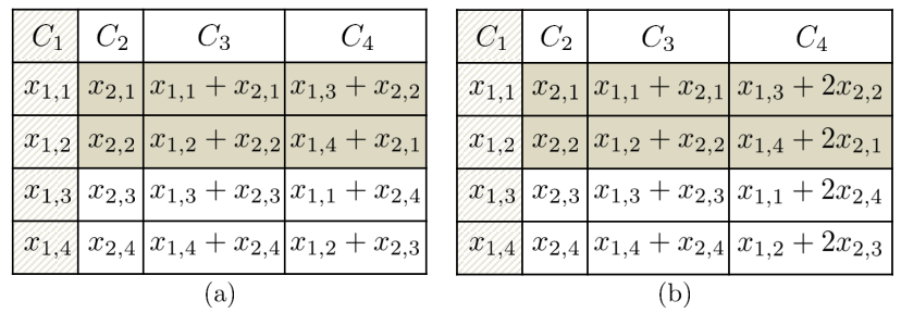
Construction II generalizes the construction given in Example II for an MSR code. Note that any MSR code construction must specify both the generator matrix of the code as well as the optimal bandwidth repair strategy that is implemented on the code.
Construction 1. Let and label the elements by -ary vectors in . Define permutation on as follows:
for and , where is the standard vector basis for . The mapping is bijective, and therefore, corresponds to a permutation on . Let be the matrix corresponding to the permutation , that is, , where , , and . In other words, scrambles the elements of a vector according to the permutation . (Notice that .)
- 1.
- 2.
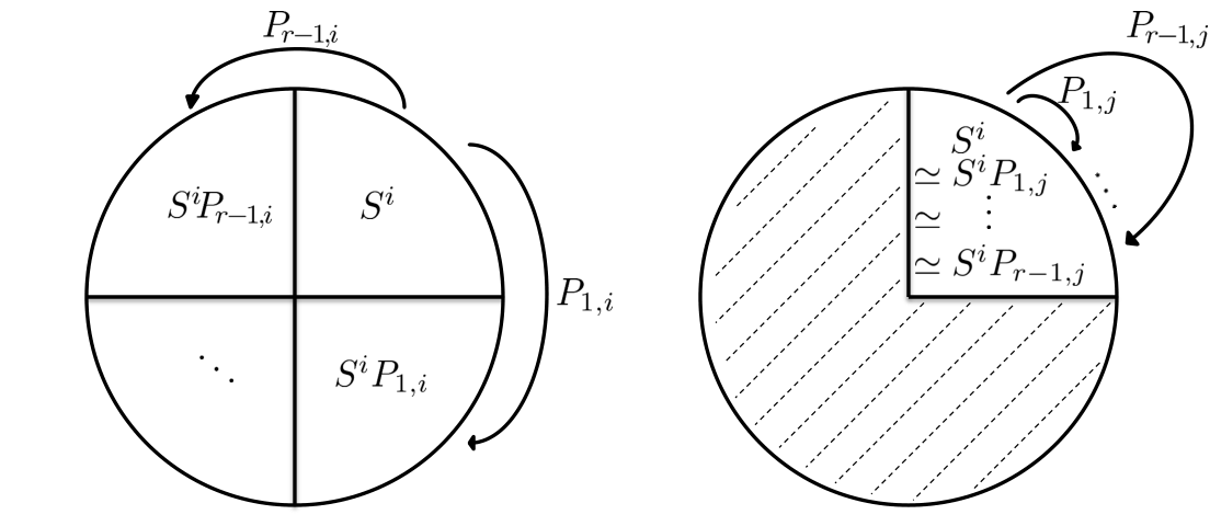
Repair Strategy: Let denote a subset of . can be interpreted as those elements in whose label representation in have a in their coordinate. If systematic node fails, it is repaired by accessing the elements corresponding to from each of the remaining nodes, i.e., by accessing , where and .
Construction II is obtained by first constructing an array code55 5 By an array code, we mean a set of systematic vectors, and parity vectors defined according to (3), which may or may not satisfy any properties. (Section II-A) which guarantees the optimal bandwidth repair for a single systematic node failure. The array code is then transformed (Section II-B) to an MDS array code (and thereby, a systematic–repair MSR code) by transforming the encoding matrices of the parity nodes, while retaining the repair property.
II-A Repair Property: Interference Alignment
The optimal repair bandwidth property of an MSR code can be viewed as a signal interference problem: the objective is to retrieve the desired signal — the contents of the failed systematic node, say, — which, in the repair data downloaded from the remaining nodes, is interfered by partial contents of the remaining systematic nodes, , where . The solution, turns out to be an interference alignment strategy, where the repair data associated with the interfering systematic data is aligned, so as to minimize the interference. This is crystallized in the following lemma66 6 This result is known and has been used in several papers on MSR codes, but we state and prove it for completeness..
Lemma 1
. Let , , be the failed systematic node. For an MSR code, the set of helper nodes is given by . To recover the contents of the failed systematic node with the optimal repair bandwidth, it is necessary and sufficient to find (repair) matrices denoted by , where , such that, for , the following two conditions are satisfied:
(a) signal recovery:
(b) interference alignment:
Stated otherwise, to optimally repair , it is necessary and sufficient to find (repair) subspaces of dimension , denoted77 7 Whenever this lemma is referenced, we use the subspace and matrix notation interchangeably as some proofs or expressions are clearer in one of the formats. We accordingly overload the notation to refer to both the matrix and the subspace spanned by the row vectors of the matrix. by , where , such that, for , the following two conditions are satisfied:
(a) signal recovery:
| (21) |
(b) interference alignment:
| (22) |
where denotes equality of subspaces, is the subspace obtained by operating the subspace by the matrix , and denotes the subspace sum.
For completeness, we provide a proof for Lemma 1 in Appendix . Lemma 2 generalizes Lemma 1 when the number of helper nodes . This will be used later in Section III.
Lemma 2
. (Corollary of Lemma 1.) In general, for an MSR code, if the set of helper nodes is given by (where denote the parity nodes in the helper set), it is necessary and sufficient to find (repair) subspaces of dimension denoted by , such that, for , the following two conditions are satisfied:
| (23) |
| (24) |
The optimal repair property of Construction II can now be justified.
Lemma 3
. The repair strategy in Construction II is optimal with respect to repair bandwidth.
Proof:
Define . Notice that the rank of subspace is . Per definition, the permutation maps to . This implies that for any distinct , the intersection contains only the all-zero vector. Thus the subspaces: , span the space () and the signal recovery condition(s) in Lemma 1 are satisfied. Furthermore, applying a permutation corresponding to a different coordinate maps to itself. This validates the interference alignment condition(s) in Lemma 1. Finally, note that the two conditions continue to be satisfied when replacing the permutations with any scaled versions , because the scaling of the basis vectors does not change the relevant subspaces and thereby does not affect the conditions in Lemma 1. ∎
II-B MDS Property
This second step relies on the following two lemmas, the proofs of which are left to the reader.
Lemma 4
. Let denote the parity part of the generator matrix for an array code denoted by , where
Given that is non-singular for all , then is an MDS array code if and only if any square sub-block-matrix of is also non-singular, where
for some .
Lemma 5
. Let denote the matrix associated with the parity part of the generator matrix for an array code, as defined in Lemma 4. Given that is non-singular for all , , and the field size is large enough, there exist coefficients , such that all square sub-block-matrices of are non-singular, where
In other words, any parity generator matrix for an array code with non-singular encoding matrices can be transformed into a parity generator matrix for an MDS array code by multiplying the encoding matrices with appropriate scalar coefficients.
Proof:
To obtain a valid set of ’s, one may first sort the pairs with respect to increasingly, and then recursively choose a value for each such that all sub-block-matrices with on their bottom right corner become non-singular. It suffices to have the field size greater than the number of such sub-block-matrices at any step multiplied by ;
∎
III Code Construction for Restricted Helper Set
We now move to the construction of systematic–repair MSR codes for any , , and , where . In this section, we start with the restricted case when the helper set includes all remaining systematic nodes. Let us begin with an example.
Example 2. Let us look at the case when for . Given a failure at the systematic node , we are interested in repairing it by downloading symbols from each node in the helper set . Let us assume that includes all of the remaining systematic nodes. Hence, there are different ways to choose depending on which two parity nodes are included in it. Let us use an indicator to differentiate between these scenarios, and denote the helper set for each scenario by .
Construction. Let and label the elements by binary vectors in . Define permutation on as follows:
for and , where is the standard vector basis for . The mapping is again bijective and therefore corresponds to a permutation on . As before, let be the matrix corresponding to the permutation , that is, , where , and . (Notice again that .)
- 1.
MSR Code: The generator matrix of the code is given by
where
(25) for . The non-zero coefficients are again selected according to the discussion in Section II-B to establish the MDS property.
- 2.
Repair Strategy via :
Let denote a subset of . can be interpreted as those elements in whose label representation in have a in their coordinate. If systematic node fails, it can be repaired by accessing the elements corresponding to from each of the helper nodes, i.e., by accessing , where and .
- 3.
Repair Strategy via :
Similarly, let . If systematic node fails, it can be repaired by accessing , where and .
- 4.
Repair Strategy via :
Finally, let denote the location of the elements that have to get accessed if the systematic node fails, i.e., node can be repaired by accessing , where and .
Proof:
Let , , be the failed systematic node. Define , , which is a product of multiple permutation matrices, and hence can be viewed as a permutation matrix itself. In order to justify the repair strategy, it suffices to define the proper subspaces that fulfill the two interference alignment conditions in Lemma 2. Let be the complimentary subset of in , i.e.,
Given the code construction in (25), we can verify that
| and, | ||||||||
| for | (26) | |||||||
Now we define subspaces . Let us for simplicity assume . The other scenarios follow the proof similarly. Based on (26), we observe that the permutation maps the basis to its complementary subset and vice versa, while preserves both of them. Hence,
Furthermore, remains unchanged under any other permutation , and hence
∎
The key element in the construction is to satisfy the two requirements in Lemma 2 for any systematic failure and any such helper set . Let denote the number of parity nodes in the helper set of size . There are different ways to choose parity nodes during the repair. Let us label these cases with numbers , and set to be the subset of parity nodes corresponding to case .
Assume that is the ordered representations, where . Finally, define -ary vectors for as
Construction 2. Let and label the elements by -ary vectors in . Define permutation on as follows:
for and , where is the standard vector basis of . Let be the matrix corresponding to the permutation .
- 1.
- 2.
Repair Strategy: Let correspond to the parity subset of the helper set . Define as . If systematic node fails, it is repaired by accessing the elements corresponding to from helper nodes, i.e., by accessing , where , and .
Lemma 6
. The repair strategy in Construction III is optimal with respect to repair bandwidth.
Proof:
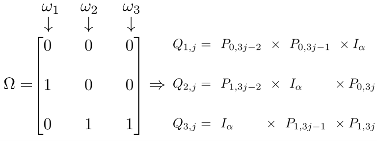
Let us first explain the role of by revisiting Example III via Figure 3. Here we assumed that
In general, the matrix is designed in a way that for any choice of we can always find a column in , denoted by , such that its intersection with rows associated with scenario , forms .
Now assume that node is failed and we are to perform an optimal systematic repair given parity repairs in . It is now clear that if we selected our subspaces as , then
and hence,
The second condition in Lemma 2 is also automatically satisfied since
∎
Lastly, we note that optimizing the sub-packetization parameter, , is not the main concern. Although Construction III suggests a fairly large value, i.e. , but it is clear that we do not need many columns in to cover all the helper set selection scenarios. Indeed, in Example III can be reduced to , where . We leave the optimizations of this kind to future work.
IV Code Construction for any Helper Set
In this section, we show that Construction III in fact holds, even when an arbitrary set of helper nodes is allowed to be chosen from the surviving nodes. This generality merely imposes some additional constraints on the selection of the scaling coefficients of the encoding matrices , where is the (product) permutation matrix corresponding to , as defined in Construction III. We now arrive at the main theorem.
Theorem 7
. Construction III gives an systematic–repair MSR code for any set of helper nodes, for a large enough field size for the scaling coefficients for the encoding matrices .
Proof:
Part 1: First, we illustrate the proof by fixing , and taking an example set of helper nodes for an example failure of node (or node ). Let us denote the (indices of the) helper set by , and let , that is, there are parity nodes and systematic nodes in the helper set. Let denote the repair information that node sends to help in the repair of node when is the set of helper nodes. (Wherever clear, we ignore the in the notation and simply write .) When node fails, the information we therefore have at its replacement node can be written as: ∎