Subgraph Counting: Color Coding Beyond Trees
Abstract
The problem of counting occurrences of query graphs in a large data graph, known as subgraph counting, is fundamental to several domains such as genomics and social network analysis. Many important special cases (e.g. triangle counting) have received significant attention. Color coding is a very general and powerful algorithmic technique for subgraph counting. Color coding has been shown to be effective in several applications, but scalable implementations are only known for the special case of tree queries (i.e. queries of treewidth one).
In this paper we present the first efficient distributed implementation for color coding that goes beyond tree queries: our algorithm applies to any query graph of treewidth . Since tree queries can be solved in time linear in the size of the data graph, our contribution is the first step into the realm of colour coding for queries that require superlinear running time in the worst case. This superlinear complexity leads to significant load balancing problems on graphs with heavy tailed degree distributions. Our algorithm structures the computation to work around high degree nodes in the data graph, and achieves very good runtime and scalability on a diverse collection of data and query graph pairs as a result. We also provide theoretical analysis of our algorithmic techniques, showing asymptotic improvements in runtime on random graphs with power law degree distributions, a popular model for real world graphs.
1 Introduction
Graphs serve as common abstractions for real world data, making graph mining primitives a critical tool for analyzing real-world networks. Counting the number of occurrences of a query graph in a large data graph (subgraph counting, often referred to as motif counting) is an important problem with applications in a variety of domains such as bioinformatics, social sciences and spam detection (e.g. [8, 10, 23]).
Subgraph counting and its variants have received a lot of attention in the literature. Substantial progress has been achieved for the case of small queries such as triangles or 4-vertex subgraphs: not only have very efficient algorithms been developed (e.g. [15, 20, 27, 31]), but also theoretical explanation of their performance on popular graph models has been obtained (see [BFMPSW14] and references therein).
Some of the recent work has addressed larger queries [29, 30, BH13, 26, 7], but our understanding here is far from complete. Even for reasonably large graphs (a million edges) and small queries (e.g. -cycles), the number of solutions tend to be enormous, running into billions. This explosion in the search space makes the subgraph counting problem very hard even for moderately large queries. Theoretically, the fastest known algorithm for counting occurrences of a -vertex subgraph in an -vertex data graph runs in time , where is the time complexity of matrix multiplication (currently ). This improves upon the trivial algorithm with runtime , but is prohibitively expensive even for moderate size queries.


To address the above issue, Alon et al. [2] proposed the color coding technique. Here, given a -node query, we assign random colors between and to the vertices of the data graph, and count the number of occurrences of the query that are colorful, meaning the vertices matched to the query have distinct colors. See Figure 1. The count is scaled up appropriately to get an estimate on the actual number of occurances. The accuracy is then improved by repeating the process over multiple random colorings and taking the average. Restricting the search to colorful matches leads to pruning of the search space and improved efficiency. Using this method, Alon et al. obtained faster algorithms for cetain queries such as paths, cycles, trees and bounded treewidth graphs.
The power of color coding as a very general counting technique together with the importance of subgraph counting in various applications (as mentioned above) makes it important to design practically efficient and scalable implementations. In a different work, Alon et al. [1] applied the color coding technique for counting the occurrences of treelets (tree queries) in biological networks. Color coding allowed them to handle tree queries up to size in protein interaction networks, extending beyond the reach of previously known approaches [25, 18, 17]. Recently, Slota and Madduri [28, 30] presented FASCIA, an efficient and scalable distributed implementation of subgraph counting (via color coding), again for the case of treelet queries. However, despite considerable interest in non-tree queries from several application domains (see the experimental section for details), the technque has not been explored for more general settings. In this work we present the first efficient distributed implementation of color coding beyond tree queries.
As part of their original color coding solution, Alon et al. [2] presented faster algorithms for certain special classes of queries. They showed that if the query is a tree, then colorful subgraph counting can be solved in time , i.e. in time linear in the size of the data graph. They extended the algorithm to show that if the query is close to a tree, specifically has (small) treewidth , a running time of can be achieved. Treewidth [9] is a widely adopted measure of the intrinsic complexity of a graph. Intuitively, it measures how close the topology of a given graph is to being a tree: tree queries have treewidth , and a cycle is the simplest example of a treewidth 2 query. The above algorithm, restricted to trees, forms the basis for the previously-mentioned treelet counting implementations [28, 30, 1].
While the runtime of the above algorithm is linear for the case of trees (i.e. acyclic queries), it becomes at least quadratic for query graphs of treewidth 2 and beyond. This phenomenon also manifests itself in practice: on real world graphs with even moderately skewed degree distribution load imbalance is observed and the running time tends to have quadratic dependence on the maximum degree of the graph. Thus, even triangles (the smallest cyclic query) are harder to handle, and have received considerable attention from the research community (as mentioned earlier).
The goal of this paper is to study the colorful subgraph counting problem on queries of treewidth , taking the first step in the realm of color coding with cyclic queries. The class of queries of treewidth is quite rich. In particular, it contains all trees, cycles, series-parallel graphs and beyond. Figure 8 shows treewidth queries (used in our experimental evaluation) drawn from real-world studies on biological, social and collaboration networks [22, 32, 4].
To the best of our knowledge, the previously-mentioned algorithm [1] is the best known algorithm for treewidth queries, and we use it as our baseline. We rephrase this algorithm within our framework and devise a distributed implementation. The rephrased algorithm becomes a recursive procedure that decomposes the query into simpler path subqueries, which are then solved to get the overall count. We thus refer to our baseline as the Path Splitting algorithm ().
Our Contributions
1. Building on the algorithm, we develop novel strategies that lead to significant performance gains in terms of runtime, scalability, and the size of graphs and queries handled.
2. Our algorithm works by decomposing the query to cycles and leaves, thereby reducing the problem of colorful subgraph counting on treewidth queries to counting (annotated) cycles.
3. The decomposition in terms of cycles enables us to exploit the so-called degree ordering approach (e.g., MinBucket algorithm for triangle enumeration [BFMPSW14]) Specifically, we show how to force the computation process to (mostly) work around high degree vertices, leading to substantial speedups and scalability gains.
4. We present a detailed experimental evaluation of the algorithms on real-world graphs having more than million edges and real-world queries of size up to 10 nodes. The results show that our strategies offer improvements of up to x in terms of running time and exhibit improved scalability.
5. Finally, we complement our experimental evalutation by a theoretical analysis of the runtime of our degree ordering approach for cycle queries, on a popular class of random power law graphs (Chung-Lu graphs [14]). Our analysis provides justification for empirically observed performance gains of the approach.
Related Work
Subgraph counting has received significant attention in the fields of computational biology [25, 18, 17] and social network analysis [21, 13, 27, BFMPSW14, 20]. We give an overview of prior work on the problem (both theoretical and empirical) as well as techniques for making subgraph counting scalable, and explain how our contributions relate to this prior work.
Color Coding and Approximate Subgraph Counting: Color coding was introduced in an influential paper by Alon et al. [2] as a fast algorithm for finding occurrences of a query in a data graph and counting the number of such occurrences. In a different work, Alon et al. [1] explored its applications to approximate subgraph counting (most commonly known as motif counting) in computational biology. They were motivated by the fact that subgraph counting is an important primitive for characterizing biological networks [MilEtAl02]. Color coding allowed Alon et al. to count occurrences of treelets (tree queries) up to size in protein interaction networks, extending beyond the reach of previously known approaches [25, 18, 17]. A scalable distributed implementation of color coding for trees has been reported by Slota and Madduri [29, 30], but no principled solutions beyond tree queries are known. ParSE [33] extends beyond tree queries, by considering query graphs that can partitioned into subtemplates via edge cuts of size 1. However, the only class of query graphs that can be perfectly partitioned using this method is trees; ParSE resorts to brute force enumeration for other cases. Our work provides the first principled approach to implementing color coding in a scalable way beyond trees queries. Further, our analysis of the runtime of our cycle counting subroutine on a random graphs with a power law degree distribution provides a theoretical justification of our algorithmic techniques.
While our work and the above-mentioned prior work [1, 29, 30] count non-induced sugraphs, some other prior work [25, 18, 17] addressed the case of counting induced subgraphs. The search space of non-induced subgraphs is larger and furthermore, these counts are more robust with respect to perturbations of the data graph [1].
Degree Based Approaches: Designing scalable subgraph counting algorithms turns out to be hard even for the simple case of triangle counting. A naive approach lets each vertex enumerate pairs of neighbors and check if they are connected. This leads to wasteful computations and also runs into load balancing issues on graphs with heavy tailed degree distributions [31]. The above issue has been addressed using a simple, but efficient solution (referred to as the MinBucket algorithm [15, 31]): each vertex enumerates pairs of neighbors with degree no smaller than its own (with arbitrary tie breaking) and checks they are connected. It is not hard to see that this gives a correct count, and it has been empirically observed that this algorithm does not run into load balancing issues even on heavy tailed graphs [31]. The MinBucket heuristic has also been shown to give polynomial runtime improvement over the naive method when the input is a random graph with a power law degree distribution [BFMPSW14]. A recent work by Jha et al. [20] applies the degree based technique for coutning -vertex queires. There are a few prior approaches for arbitrary queries of [7, 3, 26], but algorithms do not use degree information, and are comparable to the baseline algorithm used in our study.
To the best of our knowledge, prior to our work there has not been a systematic study of how MinBucket generalizes to larger subgraph counting problems. In this work we generalize the method for counting occurrences of treewidth 2 graphs, perform a thourough experimental evaluation and provide a theoretical runtime analysis of our technique in the random power law graph model. Our paper improves upon prior work along three axes: generality of queries handled, scalability of the proposed solution and theoretical analysis of the main algorithmic primitive on a class of graphs often used to model real world networks.
2 Preliminaries
Subgraph counting problem. The subgraph counting problem is defined as follows. The input consists of a query graph over a set of nodes and a data graph over a set of vertices and edges. The task is to count the number of (not necessarily induced) subgraphs of that are isomorphic to . Formally, count the number of injective mappings such that for any pair of query nodes , if , then . We refer to such mappings as matches.
Color coding and colorful matches. A coloring is a function , where for every vertex , denotes its color. A match from to is colorful if the vertices of are mapped to distinctly colored vertices in , i.e. . The main idea is that instead of counting all possible matches of the vertices of the query graph to the vertices of the data graph, one first colors the vertices of the data graph uniformly at random using colors, and then searches for colorful matches.
Colorful subgraph counting problem. In the colorful subgraph counting problem the task is to count the number of colorful matches of the query in .
Our setting counts the number of colorful matches or mappings from to the data vertices. Alternatively, we may want to count the number of colorful subgraphs that are isomorphic to . The latter quantity can be obtained by dividing the former by , the number of automorphisms of . While it is computationally hard to compute for an arbitrary query graph, the quantity can be computed quickly for queries of relatively small size (say about nodes). Given the above discussion, we focus on counting the number of colorful matches.
Treewidth. Intuitively, if the query graph has treewidth then can be decomposed into subgraphs such that each subgraph is also of treewidth , and each has no more than nodes that belong also to other subgraphs. We call such nodes the boundary nodes of . In addition, the total number of distinct boundary nodes in all subgraphs is at most . Note that the decomposition can be done recursively as each has treewidth , until we are left only with subgraphs that have at most nodes. This results in a treewidth decomposition tree denoted . A formal definition is givne below.
A tree decompsition of a query is a tree , wherein each node is associated with a subset of query nodes , called pieces, such that the following properties are true: (i) for every query edge , there exists a piece (for some ) that contains both and ; (ii) for every query node , the set of nodes whose pieces contain induce a connected subtree. Alternatively, the second property states that if belongs to pieces and for some and , then must also belong to the piece for any node found on the (unique) path connecting and in . The width of the tree decomposition is the maximum cardinality overall pieces minus one, i.e., . The treewidth of the query is the minimum width over all its tree decompositions.
Approximate subgraph counting via color coding. Counting the number of colorful matches turns out to be easier than counting the actual (not necessarily colorful) matches. The price to pay is that the algorithm is randomized. We color the graph randomly and obtain the number of colorful matches, and repeat the process independently at random a few times. Then, an estimate for the number of matches (occurances of the query) can be obtained by taking the average.
For a given input graph and query let denote the number of matches from to . For a (random) coloring of vertices of let denote the number of colorful matches of to under coloring . It was shown [2, 1] that with proper normalization the colorful count is an unbiased estimator of the actual count. Specifically, the right normalization factor is , i.e. we have . The variance of the estimator can also be bounded (see [1], section 2.1). Thus, taking the average of under a few independently chosen colorings converges to the right answer, i.e. . Thus, in order to obtain an approximate subgraph counting algorithm it suffices to solve the colorful subgraph counting problem. The rest of the paper is devoted to designing a scalable solution to colorful subgraph counting.
3 Overview
The work of Alon et al. [2] yields a natural algorithm for the colorful subgraph counting problem on bounded treewidth query graphs. This algorithm is based on the following intuition. Suppose that we have found a colorful match for a subgraph of the input query graph , and we wish to extend it into a colorful match for by additionally fixing the mapping of the nodes outside . For this we do not need to know the mapping of the non-boundary nodes of , since they do not share edges with nodes outside . Instead, it suffices to know the mapping of the boundary nodes (i.e., the nodes that share edges with nodes outside ) and the set of colors used by . The mapping of the boundary nodes is needed to ensure that for any edge from a boundary node to outside, the corresponding data vertices share an edge in the data graph; and the set of colors is needed to avoid repeating a color already used by . Analogously, in the setting of counting, in order to count the number of colorful matches for , we do not need a complete listing of colorful matches of . Instead, we can group the colorful matches based on the set of colors used and the mappings for the boundary nodes and it suffices to know the count per group.
Based on the above intuition, we apply dynamic programming to count the number colorful matches of . Let be the tree decomposition of with treewith . The algorithm processes in a bottom-up manner and a creates a hash table (that we call a projection table) for each tree node. The subgraph graph associated with a node has at most boundary nodes and these nodes can be mapped to the data vertices in at most ways. In addition, we need to record the colors of the data vertices to which the nodes of are mapped. Since we focus on colorful matches, the set of colors used (that we call “signature”) can be at most (where is the size of the query graph). For each combination of mappings to the boundary nodes and the signature, we record the number of colorful matches of consistent with the combination. The number of entries in the table is at most . The projection table for a tree node can be computed from those of its children. We get the total number of colorful matches by performing an aggregation on the projection table of the root node.
Working in the realm of motif counting, Slota and Madduri [30] described an efficient distributed implementation of the above algorithm for the case of tree queries and presented an experimental evaluation. Trees have treewidth one hence, the size of projection tables is linear in the number of vertices and the overall computation can be carried out in time linear in the graph size. Our goal is to address a more general class of queries (beyond trees) in a distributed setting and we focus on the case of queries of treewidth 2. Treewidth 2 queries are more challenging since in the worst case, the tables can be of size quadratic in the number vertices and the computation time also gets quadratic.
The construcion of our algorithm is motivated by the fact that real life data graphs tend to exhibit variations in the degree distribution. A naive implementation that treats all data vertices in the same manner would result in a lot of entries in the projection tables of the high degree vertices that do not lead to colorful matches for the overall input query. Moreover, in a distributed setting the processors owning such vertices perform more computation leading to load imbalance.
Our algorithm is based on a crucial observation that any treewidth 2 query can be recursively decomposed into (annotated) cycles or leaves. The core component of the algorithm is an efficient procedure for handling cycles that employs a strategy based on degree based ordering of vertices. This leads to reduction in wasteful computation, as well as improved load balancing. The procedure is inspired by a similar strategy used in prior work [BFMPSW14] for handling triangles. The overall algorithm uses the above decomposition and the improved procedure for handling cycles.
4 Overall Algorithm
In this section we describe the overall structure of our subgraph counting algorithm that proceeds in two steps. In the first step, we decompose the query into cycles and leaves (called blocks) and construct a decomposition tree for the input query which is essentially a carefully chosen treewidth decomposition tree; each node of the tree represents a block and encodes a convenient subquery. This step is independent of the data graph and can be viewed as a preprocessing phase for the query. Then in the second step we traverse the tree in a bottom up manner, performing primitive counting operations over the data graph prescribed by the internal nodes and combining the results. The final count is produced by the root of the tree.
4.1 Decomposition Tree
For an input query graph , construct the decomposition tree by iteratively applying one of two primitive operations: contraction of a leaf edge or a cycle. As these operations are applied the number of nodes in the query decreases. At the same time new edges may appear in to represent contracted structures, and edges as well as nodes may get annotated with the identity of the contracted structures that they represent. Before defining the tree construction algorithm we need to introduce two definitions. First, we say that a cycle in is contractible if (a) is induced (i.e. there are no edges between nodes except the edges of ) and (b) cycle has most two boundary nodes (i.e., nodes that share edges with nodes outside of ). Second, a leaf edge is an edge , where is a leaf node (has degree one); is called the boundary node of the leaf edge. We use the common term block to refer to leaf edges and contractible cycles.
For example, consider the query named in Fig 2. The cycle is contractible with a single boundary node , the cycle is contractible with two boundary nodes and , and is a leaf edge. The cycle is not contractible since it has three boundary nodes.
We construct the decomposition tree starting with an empty tree. The tree is built bottom-up starting from the leaf level and hence, the structure may be a forest with multiple roots in the intermediate stages. Each iteration adds a new node and may make some of the existing roots as its children, culminating in a tree.
In the construction process we iteratively perform the following operations until contains a single node: find a block (a leaf edge or a contractible cycle) in and remove it from (while possibly adding an edge to ), and add a corresponding node to . We iterate until contains a single node. We distinguish 3 cases.
Case 1: is a contractible cycle with exactly one boundary node : Remove the nodes and edges of from , except for node . Erase any annotation found on in and annotate it with the block name .
Case 2: is a contractible cycle with two boundary nodes : Remove the nodes and edges of from , except for the nodes and . Add an edge in and annotate it with . Erase any annotation found on and in .
Case 3: is a leaf edge : Remove and the edge from . Erase any annotation found on node and annotate it with the block name .
The nodes and edges of inherit the annotations from , as they were before was transformed (this ensures that the annotations on the boundary nodes that got erased get captured by the new annotation).
Next we add a new node to the tree . If any node or edge in has an annotation , make a child of in . This completes the construction of . We show below that the process can find a block in each iteration and terminate successfully on every query of treewidth 2. Assuming termination, it is not difficult to see that the process produces a tree. During contraction, every block annotates a particular node or an edge of , recording the way in which it has been contracted. The annotation gets inherited by some other block in a subsequent iteration. The block becomes the parent of . The annotation is erased in , ensuring that no other block becomes a parent of .
 | |||
|


Taking as the input query , Figure 2 provides an illustration process, along with the output decomposition tree. The bottom row shows the blocks being contracted and the top row shows the transformed . The first iteration contracts the cycle . A new edge is added to , along with the annotation , and is added to the tree. The second iteration contracts the leaf block . Node is annotated as and the is added to the tree. The third iteration contracts , by adding an edge with the annotation . The block is added to the tree and it is made the parent of and . In the fourth iteration, the cycle is contracted. Node gets annotated as and is added to the tree. Finally, the query is contracted leaving empty. We add as the root of the tree, making it the parent of and .
The following lemma guarantees that for any treewidth 2 query , the tree construction procedure will always find a block (a leaf edge or a contractible cycle) in each iteration and terminate successfully. The proof relies on prior work on nested ear decompositions of treewidth 2 queries [16].
Lemma 4.1
(i) Any treewidth 2 query contains a block; (ii) the transformed query resulting from the contraction process is also a treewidth 2 query.
Proof: We first prove part (ii) of the lemma. If the contracted block has one boundary node then no new edges are added to , in which case the tree for the updated is given by deleting all the nodes not in the updated from the subsets . If the contracted block has two boundary nodes and then the edge is added to . In this case we get the tree for the updated by replacing each occurrence of the nodes not in the updated by . Note that the size of each subset is still at most 3, nodes associated with subsets that contain form a connected component, and for at least one subset , .
We now prove part (i). First, Root the tree at an arbitrary non-leaf node. This induces an ancestor-descendant relationship on the nodes in . Note that if there are two nodes , such that , node can be omitted and all its children connected to . Thus from now on we assume that no subset is contained (or identical) to another subset.
We need the following definition and claim.
Definition 4.1
For a node , let be the subgraph of induced by the nodes that are in the union of the subsets associated with the nodes of in the subtree rooted at .
Claim 4.1
For every node , either contains a block, or is a path whose endpoints are in the subset associated with the parent of (if such exists).
Before proving the claim we show how it implies the lemma. Since the claim holds also for the root of then either contains a block or it is a path in which case it also contains a leaf block.
Proof of Claim 4.1: We prove the claim by induction. The base of the induction is a leaf node. Consider a leaf node . There are two possibilities: (i) , and (ii) . If , then at least one node, say , is only connected to and thus is a leaf edge.
If , then consider the subgraph induced by . If this subgraph is a triangle then it must be a contractible cycle. The only remaining case is the subgraph induced by forms a path. Assume that the endpoints of this path are and . If one of these endpoints, say , is not in the subset associated with the parent of then is a leaf edge. Otherwise, let be the parent of , we have .
For the inductive step consider a non-leaf node . If for any child of contains a block then we are done. Assume that this is not the case. Consider first the case that has a single child . By the inductive hypothesis is a path whose endpoints and are in . Let . If is connected to both and then the cycle closed by is a contractible cycle. If is connected to only one endpoint, say , then we get a path with endpoints and . If either or are not in the subset associated with the parent of , then the missing endpoint is leaf node. If both and are in the subset associated with the parent of then the inductive claim follows.
Next, Consider the case that has several children. If two of the children of , say and , share endpoints then the cycle formed by and is contractible. Otherwise, must have exactly two children, say and , with endpoint and , forming a path with endpoints and . If is connected also to then the cycle closed by the edge is a contractible cycle. If either or are not in the subset associated with the parent of , then the missing endpoint is a leaf node. If both and are in the subset associated with the parent of then the inductive claim follows.
An input query may admit multiple decomposition trees and the choice of the tree influences the performance of our algorithm. In Section 6, we present a heuristic for finding a good decomposition. Each node of the tree represents a block and it will be convenient to view to the node simply as the block represented by it.
At this point, it is interesting to consider tree queries studied by Slota and Madduri [30]. Given a tree query, their algorithm fixes a suitable query node as the root and iteratively processes the tree in a bottom-up manner. The algorithm implicitly uses a decomposition tree. However, since trees do not have cycles, the decomposition tree consists of only leaf edge blocks. In contrast, the decomposition trees of treewidth two queries involve the more challenging case of cycles as well.
4.2 Tree Traversal
Here, we describe the second step of the algorithm that traverses the decomposition tree in a bottom-up manner and computes the number of colorful matches of the blocks in the data graph. For this purpose, we define the notion of subqueries represented by blocks.
A subquery of the input query refers to any induced subgraph of . Consider a block and let be the union of nodes found in the block and its descendant blocks in the tree. The subquery represented by , denoted , refers to the subquery induced by . For example, Figure 2 shows the subquery represented by the block . The decomposition tree yields a nested hierarchy of subqueries: the root block represents the whole input query and for any block with the parent , the subquery is contained within .
Let be a block. A node is said to be a boundary node, if shares an edge with a node outside . It is not hard to see that these boundary nodes are the same as the boundary nodes of (identified during the tree construction process). Thus, can have at most two boundary nodes.
Before describing the counting algorithm we extend the notion of colorful matches to subqueries: a colorful match for a subquery is an injective mapping , such that for any edge , , and the vertices of are mapped to distinctly colored vertices of .
The algorithm traverses the tree in a bottom-up manner. For each block , it outputs a succinct synopsis of the set of colorful matches of the subquery , using a projection table and signature (as outlined in Section 3). that we now define precisely.
Signature: Let denote the set of colors used in the data graph, where is the size of the input query . The term signature refers to any subset . For a subquery and a colorful match of , the signature of refers to the set of colors of the data vertices used by and it is denoted , i.e., .
Projection Tables: Let be subquery with two boundary nodes and . For a pair of data vertices and and a signature let denote the number of colorful matches of wherein the boundary nodes and are mapped to and and the signature of is :
where is the set of all the colorful matches of .
These counts can be conveniently represented in the form a hash table with forming the key and the count forming the value. We refer to any encoding of the above counts (such as the hash table above) as the projection table of . In the worst case, the table may have size quadratic in the input data graph. However, a significant fraction of the triplets will have a count of zero and we maintain only the non-zero counts.
The projection table for subqueries having a single boundary node is defined in a similar manner. For a data vertex and a signature , define
Overall Algorithm 1. Compute a decomposition tree for the input query . 2. Traverse the tree bottom-up. For each non-root block : Use the projection tables of the children blocks of and compute the projection table for 3. Output the number of colorful mathes of the subquery represented by the root-block.
4.3 Computing the Counts
Given a decomposition tree, the algorithm works based on the fact that the projection table for a block can be computed by joining the projection table of its children blocks.
As an illustration of the idea, consider the block having boundary nodes and , and the subquery represented by it (Figure 2). For a pair of vertices and , and a signature , the projection count can be computed as follows. The block consists of the path , and any match for the subquery must map these nodes to vertices that form a path in the data graph. The block is annotated by its children blocks with boundary nodes and , and with boundary node . Any pair of matches and for and can be extended as matches for , as long as their signatures and are disjoint (since the blocks do not share any node) and are contained within . Therefore, we can derive the desired count by performing the following aggregation over all quadruples satisfying the properties: forms a path in the data graph; ; is empty. The aggregation is:
We can express the projection counts for any block in the above manner. However, as the number of children increases, the cartesian product involved in the aggregation would be prohibitively expensive. Our procedures efficiently simulate the aggregation by performing a sequence of join operations involving the projection tables of children blocks.
Given a decomposition tree, the algorithm traverses the decomposition tree in a bottom-up manner, computing the projection tables for all the blocks and culminates in the root-block representing the whole input query. At this step, instead of producing a projection table, the algorithm simply computes the number of colorful matches. The pseudo-code is shown in Figure 3.
5 Solving Blocks
The main step of the algorithm is the construction of the projection tables of a block from its children blocks. In this section we develop efficient procedures for handling cycles. For the sake of highlighting the main ideas, we first focus on the case of cycles found at a leaf level of the decomposition tree (such as the cycle in Figure 2); these cycles do not have other blocks annotating them. General cycles are handled by extending these ideas as discussed later.
5.1 Solving Cycles at the Leaf Level
Consider a cycle block of length without annotations. The cycle may have at most two boundary nodes. We discuss the more interesting case where the number of boundary nodes is exactly two; the other cases are handled in a similar fashion. Let the two boundary nodes of the cycle be and , for some . We present two procedures for computing the projection table of : a baseline procedure that uses a path splitting strategy and an efficient procedure guided by a degree based ordering of vertices.
Procedure 1: Computing Projection Table for For each edge in the data graph , where . For For each triple with For each edge in such that do: Let . Increment by . Procedure 2: Computing Projection Table for For each entry with For each entry with If ; Increment by .
Path Splitting Algorithm (). For two nodes and on the cycle, let and be the paths obtained by traversing the cycle from to in the clockwise and counter-clockwise directions, respectively, i.e., and , where and refer to addition and subtraction modulo .
Let denote the projection counts for path taking and as the boundary nodes. Namely, for a triple , let denote the number of colorful matches for wherein , and . A similar notion is defined for the paths .

The procedure splits the cycle into two paths along the boundary nodes, given by and ; we refer to these special paths as and . See Fig 5 (a) for an illustration.
The projection table for is constructed iteratively, by building the tables for the paths , for each node found along the path. This is accomplished by extending the projection table for the prior path via a join with the edges of the data graph. The pseudocode is given in Figure 4 (Procedure 1). We assume that all the counts are initialized to zero. The first iteration is handled by directly reading the edges of the data graph. In the subsequent iterations, we extend every triple with non-zero count , with any edge , provided the resulting match is colorful. The counts for are constructed analogously. Finally, the projection table for the cycle is obtained by joining the counts of and , as shown in Procedure 2. Here, a pair of triples and are joined, if the resulting match is colorful.
Discussion of baseline. As discussed below (Section 5.2), the procedure can be extended to handle general cycles with annotations, and yields an algorithm for handling treewidth 2 queries. The resultant algorithm is equivalent to the original color coding algorithm of Alon et al. [2]. Prior work [30, 1] on colorful subgraph counting utilize the algorithm of Alon et al. as the basis for counting tree queries (treelets). We developed a distributed implementation of the algorithm, and use it as the baseline in our experimental study. Known techniques for subgraph counting with large queries (e.g. [7, 26]) employ similar graph traversal techniques, making PS consistent with the state of the art for subgraph counting as well as color coding.
We develop an procedure, called Degree Based (DB) algorithm, that outperforms the algorithm for practical graphs and queries. It is motivated by the following observations. First, the paths and may have uneven lengths (for instance, in Figure 5), and ) and the processing of the longer path dominates the overall running time. Second, in real-graphs with skewed degree distributions, high degree vertices tend to have more paths passing through them, which populate the projection tables of and . However, significant fraction of these paths do not find appropriate counterparts in the other table to complete a match, leading to wasteful computations. Third, in a distributed setting, the above phenomenon manifests as higher load on processors owning high degree vertices, leading to load imbalance.
It is not difficult to address the first issue alone. The only intricacy is that when the paths are split evenly, the boundary nodes may appear internally on the the paths (see Figure 5 with a split across nodes denoted and ). This can be handled by recording the mapping for the boundary nodes as part of the projection counts. We implemented the above algorithm as well and noticed that the issue of wasteful computations and load imbalance still persists. And furthermore, performance of the algorithm and the modified implementations does not differ significantly on our benchmark graphs and queries.
Degree Based Algorithm ). The algorithm addresses all the three issues by using the strategy of building the paths from high degree vertices.
Arrange the data vertices in the increasing order of their degree; if two vertices have the same degree, the tie is broken arbitrarily, say by placing the vertex having the least id first. We say that a vertex is higher than a vertex , if appears after in the above ordering and this is denoted “”.
Consider the input cycle with boundary nodes and and let be a colorful match for that maps the above nodes to data vertices , respectively. Among these data vertices, let be the highest vertex. We refer to the corresponding node as the highest node of .
The idea is to partition the set of colorful matches into groups based on their highest node and compute the projection table for each group separately. For a pair of data vertices and , and a signature , let denote the number of colorful matches of for , wherein , , and is the highest node of . The projection table for can be obtained by aggregating the above counts: for any triple ,
| (1) |
We next describe an efficient procedure for computing the counts . The concept of high starting matches plays a crucial role in the procedure. Let be the node diagonally opposite to on the cycle, i.e., . The procedure splits the cycles into two paths and ; Figure 5 (b) shows the paths for two sample values of . Let be a node found on the path , A colorful match for is said to be high-starting, if the data vertex is higher than all the other data vertices used by , i.e., , for all nodes on the path . For a pair of vertices and , and a signature , let denote the number of high-starting colorful matches for the path wherein , and .
We then count the high-starting colorful matches for the two paths, which can be accomplished via edge extensions, as in the algorithm. However, the current setting offers a crucial advantage: we can dictate that the starting node is the highest node, meaning whenever an entry gets extended by an edge , we can impose the condition that is higher than in the degree based ordering. Imposing the condition leads to a significant pruning of the tables. The pseudo-code is given in Figure 6 (Procedure 1).
Procedure 1: Compute For each edge in the data graph with , where . For For each triple with For each edge in s.t. and : Let . Incr. by . Procedure 2: Compute for Config. (A) For each entry with For each entry with If ; Incr. by .
While the degree based strategy is more efficient, we need to address an intricacy regarding the projection aspects. In contrast to the algorithm, the algorithm splits at the highest node and consequently, the boundary nodes and may appear inside the paths. Thus, in order to get the projection counts on and , we also need to explicitly record the mappings for the boundary nodes.
The two nodes and may occur on either or . Six different configurations are possible, of which two are shown in Figure 5 (b). In Configuration (A), the paths include one boundary each, whereas in the second configuration, the same path includes both the boundary nodes. The other four configurations are symmetric: the boundary nodes may swap the paths in which they occur and in Configuration (B) can also reverse the order in which they occur. We discuss the two configurations shown in the figure; the other configurations are handled in a similar fashion.
Consider configuration (A). In order to record the mappings of the boundary node , we introduce an additional field in the projection counts. For a triple of data vertices , and , and a signature , let denote the number of high-starting matches for with , , and . These counts are computed in a manner similar to the base procedure shown in Figure 6 (Procedure 1); however, when the process encounters the boundary node (namely, the initialization step or ), the mapped vertex ( or , respectively) is recorded in the additional field. The analogous counts for can derived in a similar manner. The value of is obtained by joining the two; see Procedure (2) in Figure 6. Configuration (B) is handled in a similar fashion, except that we need two additional fields to record the mappings for both the boundary nodes. Namely, we maintain counts having keys of the form representing the mapping of the nodes and to the vertices and . Procedure (2) is also adjusted accordingly. Finally, we can get the projection table via aggregation, as in Equation 1.
Compute Projection Table for Let be the block annotating the edge For Execute ) Execute ) Execute : If is annotated by a block For each with For each with If ; Incr. by For each entry For each entry and If ; Incr. by
5.2 Solving General Blocks
In this section, we present procedures for handling generic blocks. We first consider the case of cycle blocks with two boundary nodes.
Consider a generic cycle having two boundary nodes and , whose nodes and edges may be annotated with other blocks (children of in the decomposition tree). All these blocks have at most two boundary nodes and these are found on . For such any block , the subquery represented by has the same boundary nodes as that of . Thus, we can get the projection table for by joining the projection tables of the subqueries represented by the above blocks, as described below.
As before, we consider each possible choice for the highest node and split the cycle into two paths and . The path segment also represents a subquery (induced by the union of the nodes found in the path and the blocks annotating path). Thus, we can extend the notion of projection tables for these segments as well. The procedure for computing the projection table for is similar that the one discussed in previous section (Procedure 1 in Figure 6), and works by extending one edge in each step. However, two aspects need to be addressed. Firstly, in contrast to the prior procedure, the edge being extended may be annotated with a block or un-annoated (and correspond to an original edge found in input query ). In the former case, we perform a join operation with the edges of the data graph (as before), whereas in the latter case the join operation involves the projection table of the block . For the sake of uniformity, it will be convenient to view the former edges as blocks as well, denoted , and associate with them a projection table derived from the graph edges, as follows. For each edge , set as , for ; all other entries of the table are set to a count of zero. The second aspect is that the nodes of the cycles may also be annotated, and these get included as part of the sequence of joins being performed. The two aspects are addressed by procedures called NodeJoin and EdgeJoin. The pseudo-code is shown in Figure 7.
The procedure starts with an initial table representing the first edge and performs a sequence of join operation with the blocks annoatating the nodes and edges of the cycle. At this juncture, two intricacies must be highlited. Firstly, the endpoint and/or may be annotated by a block , which must be joined by either or , but not by both (to avoid double counting). For this purpose, we adopt the convention that and include only the block annotating and (if found), respetively. Secondly, for a block with two boundary nodes and , the projection table views one of them as the first boundary node and the other as the second (corresponding to the two components of the keys of the form ). Thus, the boundary nodes are ordered and the projection tables need not be symmetric: taking as the first boundary node and as the second boundary node would produce a different boundary tables. However, the boundary tables are transpose of each other (). Our algorithm maintains both the tables and uses the appropriate one as dictated by the nodes of the cycle. The pseudo-code reflects the first aspect, but, for the sake of clarity, ignores the second.
The projection counts obtained by the above process are joined using a proecure similar to Figure 6, taking into account the configuration in which the boundary nodes occur. These are aggregated over all possible choices of the high node .
Cycles with a single boundary node are handled in a similar manner by considering each possible choice for the highest node and splitting the cycle into two paths and . The setting is simpler with only two configurations possible on how the boundary nodes may appear on the paths: the (single) boundary node may appear in or . Thus, the prior procedures can be applied here as well.
The case of leaf blocks are also handled via join operations. Any leaf block is processed by joining the projection table for the blocks annotating the nodes , the edge and the node (if found).
At the end of the traversal process, the root block is solved, which is either a cycle or a singleton node. In the former case, the block is treated as a cycle without boundary nodes. Instead of computing its projection table, we simply count the number of colorful matches, via a procedure similar to that of two-boundary cycles. In the latter case, we consider the projection table of the block annotating the singleton node and output the sum of counts across all entries of the table. The process yields the number of colorful matches of the input query .
6 Finding Good Decomposition Trees
In each step of the decomposition process, multiple blocks may be available for contraction. Each sequence of choices leads to a unique decomposition tree, and hence, multiple trees are possible for a given query. For example, the query (Figure 8) admits two decomposition trees: (i) contract the -cycle first and then the -cycle, and (ii) vice versa. We conducted an experimental study involving a number of real-world data graphs and queries. For each query, we enumerated all the possible decomposition trees and evaluated the execution time on each graph. We observed a maximum difference of x in the execution times of two decomposition trees for the same graph-query combination. However, we noted that in most cases the optimal tree is independent of the data graph and is mainly determined by the structure of the query. These observations show that we need a procedure for selecting a good tree, but in this process, we need not analyze the large data graph; rather, it suffices to focus on the structural properties of the small query graph.
Our study also showed that the following factors, in the decreasing order of importance, determine the execution time: (i) length of the longest cycle block; (ii) number of boundary nodes; (iii) number of node/edge annotations. Armed with the above observations, we designed a simple heuristic procedure. Enumerate all possible trees for the given query and pick the best using the above factors for comparison. In our experimental setting, barring a few exceptions, the heuristic picked the optimal tree in majority of the cases and a near-optimal tree for the rest. Since the queries are of small size (about 10 nodes), even a sequential implementation of the heuristic takes insignificant amount of running time.
7 Distributed Implementation
In this section, we present a brief sketch of the distributed implementation of the two algorithms, highlighting their main aspects. The distributed implementation consists of three layers. The first layer, called the planner, finds a good decomposition tree for the given query a fast sequential implementation the heuristic discussed in Section 6. The second layer, called the plan solver, takes the data graph and the decomposition tree and implements the and algorithms presented in Section 5. It accomplishes the above task by using efficient join routines supported by the third layer, called engine. The engine has three functionalities. The first is to store the data graph in a distributed manner. This is achieved via a decomposition, wherein the vertices are equally distributed among the processors using block distribution, and each vertex is owned by some processor. The second is to maintain projection tables. These tables are of two types: unary projection tables having single-vertex keys of the form associated with blocks having single boundary nodes; binary projection tables having two-vertex keys of the form . The binary tables also have variants involving additional fields for storing the mappings for the boundary vertices. The engine provides a convenient abstraction to the plan solver for all these types of tables. All the tables are maintained as distributed hash tables which use open addressing to resolve collisions. Every entry is stored on the processor owning ; the degree of is packed as part of the entry for enforcing the degree constraint in the join operations (of the form in Procedure 1 of Figure 6). Signatures are maintained as bitmaps. The third functionality is to support two types of join operations on the projection tables. The first type of join is used for extending a path segment an edge; this involves a join with either the graph edges or the projection table of the block annotating the edge. In the former case, the extension of an entry with a key with an edge will be performed at the owner of . The result is an entry with a key ; this entry is communicated to the owner of , where it gets stored. The latter case involves join of two entries with keys and . Since the first entry is stored at the owner of and the second, at the owner of , a communication is performed to bring the two entries to a common processor. The second type of join is used for merging the projection tables of two path segments (for example, Procedure 2 in Figure 6) and it is implemented in a similar way. The two operations are implemented using a standard sort-merge join procedure with signature compatibility checks performed via fast bitwise operations.
| Graph | Domain | Nodes | Edges | Avg | Max |
| Deg | Deg | ||||
| brightkite | Geo loc. | 58K | 214K | 4 | 1135 |
| condMat | Collab. | 23K | 93K | 4 | 281 |
| astroph | Collab. | 18K | 198K | 11 | 504 |
| enron | Commn. | 36K | 180K | 5 | 1385 |
| hepph | Citation | 34K | 421K | 12 | 848 |
| slashdot | Soc. net. | 82K | 900K | 11 | 2554 |
| epinions | Soc. net. | 131K | 841K | 6 | 3558 |
| orkut | Soc. net. | 524K | 1.3M | 3 | 1634 |
| roadNetCA | Road net. | 2M | 2.7M | 1.3 | 14 |
| brain | Biology | 400K | 1.1M | 3 | 286 |

8 Experimental Study
We present an extensive experimental evaluation of the algorithms presented in the paper. Our experiments include a comparison of the algorithms on execution time, strong and weak scaling studies for our algorithm, and studies to evaluate the quality of our query plan generation heuristic and the efficacy of color coding for treewidth two queries.
8.1 Experimental Setup
System. The experiments were conducted on an IBM Blue Gene/Q system [12]. Each BG/Q node has cores and GB memory; multiple nodes are connected using a D torus interconnect. Our implementation is based on MPI2 with gcc 4.4.6 with the number of ranks varying from to . Each MPI rank was mapped to a single core. The number of MPI ranks mapped to a node was adjusted based on the memory requirements of individual experiments.
Graphs. The experiments involved nine real world graphs obtained from the SNAP dataset collection and the human brain network from the Open Connectome Project (http://snap.stanford.edu, http://www.openconnectomeproject.org/). Our benchmark includes representative graphs from different domains in SNAP. The graphs and their characteristics are presented in Table 1. We also used synthetic R-MAT graphs [11], for the purpose of studying the weak scaling behavior of our algorithms.
Queries. Our query benchmark consists of the ten real world queries shown in Figure 8. The queries were derived from prior network analysis work spanning diverse domains: dros, ecoli1, ecoli2, brain1, brain2, brain3 - biological networks [22, 19]; glet1, glet2 - graphlets [7]; wiki - collaboration networks [32]; youtube - spam networks [24].
Algorithms. We study two algorithms: , which serves as the baseline, and our degree based algorithm. Recall that is equivalent to the dyamic programming based algorithm of Alon et al. [2].

8.2 Graph-Query Characteristics
The characteristics of the input graph and query strongly influence the running time of query counting algorithms. To obtain an overall characterization of the phenomenon, we measured the execution time of the algorithm on each of the 100 real graph and query combinations using 512 MPI ranks. Figure 9 shows the average running time for each graph across the ten queries and the average running time of each query across the ten graphs. The wide variations in execution time across graphs and queries is indicative of their relative difficulty in practice. For example, although roadNetCA is a larger graph than epinions, the average running time of the former is smaller than the latter by an order of magnitude. We can understand this behaviour by studying the skew in underlying degree distribution. In general, counting colorful occurrences of a query on a graph with high skew (indicated by high maximum degree in Table 1) tends to be computationally expensive. Similarly, the queries also exhibit large variations in running time, ranging from sub-second for youtube, glet1 and glet2 to more than a minute for brain2 and brain3. These variations can be accounted for by studying the differences in the size and the sub-structures of the queries. We observed that queries with longer cycles are more challenging. As an extreme case, a -vertex complete binary tree query requires 2 seconds on average, in contrast to the -vertex brain3 query which requires nearly 2 minutes on average, exemplifies our observation.
8.3 Performance Comparison of and Algorithms
We study the performance of the and algorithms on 100 graph-query combinations obtained by selecting a graph from Table 1 and a query from Figure 8. For our algorithm, we used plans supplied by the heuristic described in Section 6. In contrast, for the algorithm, we enumerated all the possible plans and obtained the optimal plan. Thus, we compare our algorithm to the best possible scenario for the baseline algorithm.
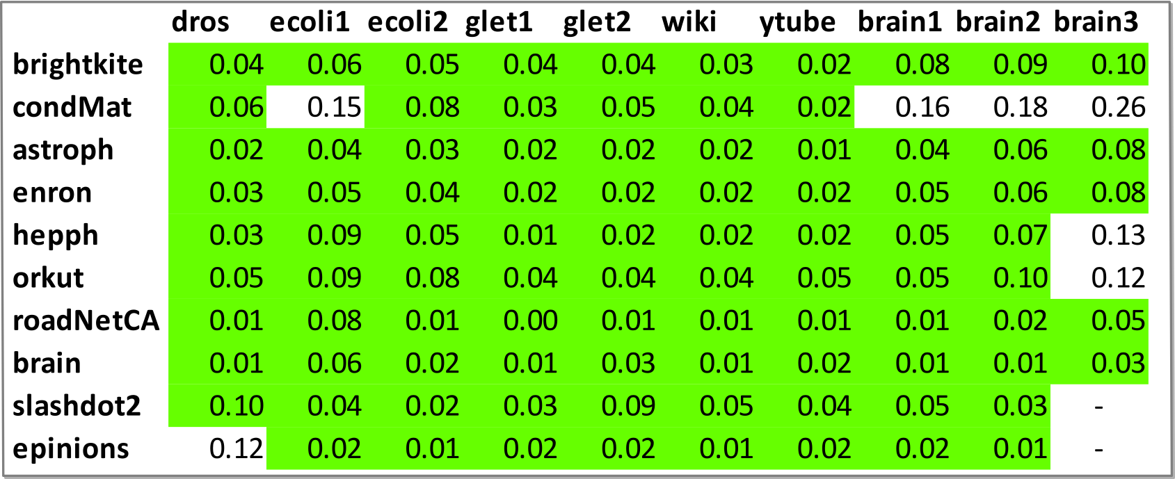
We compute the improvement factor of over as the ratio of the execution time of to . Figure 10 shows at and ranks. The combinations where outperforms are highlighted in green. The blank entries represent cases where (or ) did not complete execution, due to lack of available memory. At ranks, we can see that outperforms on 84% of the graph-query combinations with being as high as x (average x). At ranks, outperforms the baseline on 89 of the cases, with becoming as high as x (average x).
 |
| (a) Ranks |
 |
| (b) Ranks |
We can see that the relative performance of the two algorithms is dependent on the graph-query pair. For instance, the average on enron and condmat graphs are and on ranks, respectively, correlating well with their skew in the degree distribution (see Table 1). Similarly, the improvement factors is higher on complex queries such as brain1 where the average improvement is x, compared to youtube where the average improvement is only x. The phenomenon becomes extreme in the case of road networks that have very low skew and exhibit sub-second average running time across queries.
Our algorithm scales better than , as demonstrated by the increase in at higher ranks. For different graph-query combinations, we computed the ratio of at ranks to that of ranks and found that increases by a factor of up to x (average x). To understand this trend further, we compute the load (number of projection function operations) for both algorithms for processing different queries on the enron graph at 512 ranks. For different queries, Figure 11 shows the execution time and the average and maximum load. We can see that has lesser average load than , since avoids wasteful computations. Furthermore, the improvement obtained by over on execution time correlates well with improvement obtained on the maximum load. For example, on ecoli1 query, even though outperforms at ranks, the perforamance is reversed at ranks (see Fig 10), because of superior load balancing characteristic of .
| ||||||
| (c) Avg. Load |

8.4 Scalability Characteristics of Algorithm
We studied the scaling of across the 100 graph-query combinations. For each combination, we computed the ratio of the execution time at ranks to that of ranks. Figure 12 summarizes the above information by providing the averge of the above speedup for each query across graphs and the same for each graph across queries. As against an ideal speedup of x, we see that the algorithms obtains speedups in the range of x to x.
We studied the strong scaling behavior of our algorithm, using enron as a representative graph. Taking ranks as the baseline, Figure 13 shows the speedup up to ranks for different queries. The algorithm scales well across queries, with an average speedup of x and maximum speedup of x at ranks (as against an ideal speedup of x).
To study weak scaling, we use R-MAT synthetic graphs with parameters , , and and edge factor , suggested in a Graph 500 benchmark specification (http://www.cc.gatech.edu/~jriedy/tmp/graph500/). The number of vertices was fixed at per rank and the number of ranks was varied from 32 to 512. We report the execution times each query-rank combination in Figure 13. We see excellent weak scaling behavior with the execution times at ranks remaining close to that of the baseline 32 ranks.
8.5 Evaluation of Plan Generation Heuristic
We studied the quality of our plan generation heuristic for the algorithm at ranks. For each graph-query combination, we determined the optimal plan via an exhaustive enumeration. We compared the execution time of the heuristic plan to the optimal plan and measured the percentage difference. These results are reported in Figure 14. We can see that in % of the case, the heuristic generated the optimal plan, whereas in the remaninig cases, the difference was at most %.
8.6 Precision of Color Coding
We evaluated the precision of color coding on our benchmark by performing independent trials and computing the empirical variance of the sample (see Section 2). Specifically, for a given graph-query combination we performed a sequence of trials, where in each trial the colorful count was computed for a fresh random coloring. We performed 10 random trials for each of the 100 graph-query combinations in our test set and evaluated the empirical mean and variance of the number of colorful matches. For each graph-query combination, we computed the coefficient of variation, which is the ratio of the empirical variance to the mean. The results are shown in Figure 15. A value close to 0 indicates the convergence of our estimate to the true mean . We observed that with only three trials, 82% of the graph-query combinations had coefficient of variation at most ; when the number of trials was increased to 10, it increases to 91%. Hence, using 512 ranks, for a majority of the input graph-query combinations in our benchmark, we require less than a minute to count the actual number of matches of the query, with accuracy. We conclude that our algorithm enables fast approximate counting of treewidth 2 queries for data graphs spanning various real domains.

9 Cycle queries on random power law graphs
In this section we concentrate on cycle queries of constant size and analyze the expected runtime of a variant of the PS and DB procedures on a certain class of random data graphs. We prove a lower bound on the expected runtime of the PS procedure and an upper bound on the expected runtime of the DB procedure. Both bounds are functions of the (expected) degree sequence of the graph. We show that our upper bound on the runtime of the DB procedure is never worse (up to constant factors) than the lower bound on the PS procedure. Moreover, if the random graphs satisfy a natural power law property then we prove that the expected runtime of the DB procedure is polynomially better. Recall that the most complicated blocks in our general decomposition of the query graph are (annotated) cycles. Thus, we postulate that the better performance of our variant of the DB procedure on cycle queries explains the better performance of the DB procedure studied in the main body of the paper on queries of treewidth 2.
The class of random graphs considered is a certain variant of the Chung-Lu graphs [14], a popular model for random graphs that captures several properties of real world social networks, as defined precisely below.
9.1 The procedures analyzed
Consider a cycle query of constant size . Since the query graph is a cycle, the decomposition tree consists of only a root node which represents this cycle with a single boundary node.
Recall that procedure PS computes , for each node . For this it first computes and for all of nodes and all signatures. Since is constant the number of signatures is also constant and thus computing given and can be done in linear time. In the PS procedure the computation of and is done by iteratively recomputing for all and . This recomputation can be viewed as a optimized version of enumerating all paths starting at , where instead of storing paths explicitly, we only store the two endpoints, the signature, and a count. Our simplified variant of the PS procedure, which is more amenable to analysis, computes and by enumerating all possible paths, instead of performing this optimized enumeration. Thus, its complexity is linear in the number of possible paths of lengths . We will refer to this version of PS procedure as the PS procedure throughout this section to simplify notation.
To increase the efficiency of our PS procedure when applied to cycle queries we can break symmetry using the id of the nodes and count only colorful matches where node has the largest id among all data nodes in the image of . Consequently, and need only to count paths with the property that node has the largest id among nodes on the path.
For an integer let
| (2) |
It follows that the expected complexity of procedure PS is linear in . Later, we derive lower bounds on for any constant , and our bounds are monotone increasing in . Thus, the dominant term in the complexity of procedure PS is provided by our bound on .
Procedure DB also computes , but does it by computing high-starting colorful matches. Again, to increase the efficiency of procedure DB when applied to cycle queries we can break symmetry and only compute , namely, colorful matches where node is the highest in the degree based ordering among all data nodes in the image of . It follows that for this we need only to compute and , namely, the number of high-starting colorful matches for the paths and , wherein , and , for all possible and . Note that similarly to the PS procedure, the recomputation in the DB procedure considered in the main body of the paper can be viewed as a optimized enumeration, where instead of storing paths explicitly, we only store the two endpoints, the signature, and a count. Our simplified variant of the DB procedure, which is more amenable to analysis, computes the counts by enumerating all these paths, instead of performing this optimized enumeration.
For an integer let
| (3) |
It follows that the expected complexity of procedure DB is linear in . Later, we will derive bounds on , and since our bounds will be monotone increasing in , the dominant term in complexity of procedure DB is provided by our bound on .
9.2 The random data graphs
We analyze our algorithm on Chung-Lu graphs whose expected degree sequence has some additional property.
Chung-Lu distribution
The Chung-Lu distribution on random graphs is defined as follows. First choose a degree sequence , where . We assume that for all . Let . We assume that and . To generate the graph we include each edge independently with probability . Note that the expected degree of every node is as required. We write to denote the actual degree of in .
We require the degree sequence to be -balanced.
Balanced degree sequence
A degree sequence is -balanced for some if for any integers , . Intuitively, a degree sequence is balanced if it is not too concentrated on the high degree nodes.
For some of the claims we require the sequence to satisfy the stronger truncated power law.
Truncated power law distribution
A degree sequence satisfies the truncated power law for a constant if for each , the number of nodes with degree between and is . We show later that if a sequence satisfies the power law for then it is -balanced for .
9.3 Main theorem
Theorem 9.1
Let be sampled according to the Chung-Lu distribution on vertices with an -balanced degree sequence , for some constant , and let be a constant. Then,
- (1)
-
The expected number of paths of length for which is with the highest id is lower bounded by
- (2)
-
The expected number of high-starting paths of length is upper bounded by
for some constant .
- (3)
-
Based on the above inequalities
- 1.
.
- 2.
If the degree sequence satisfies the truncated power law with parameter , for any constant , then is polynomially smaller than .
- 1.
Proof: (1) follows by Lemma 9.5. (2) follows by Lemma 9.6. (3) follows by putting together Lemma 9.7 and Lemma 9.8.
Remark 9.2
Note that if and , since by our assumption on the degree sequence. Thus both and are monotone in . It follows that for any constant , the dominant terms in the complexity of our PS and DB procedures for query cycles of length is indeed determined by and , respectively, as claimed in section 9.1.
9.4 Useful facts
In this section we state some simple claims and known results that will be useful in the rest of the proof. The following claim specifies the probability that a fixed path exists in a random graph drawn from the Chung-Lu distribution:
Claim 9.1
Let be drawn from the Chung-Lu distribution with degree sequence . Then for any and a vector of distinct nodes
Proof: Since the input graph is drawn from the Chung-Lu distribution, for each we have
Since edges are included in independently, we have
We will also use
Theorem 9.3 (Chernoff bound)
Let be independent Bernoulli random variables. Let , and let . Then for any
and for every
A simple corollary of the bound is
Corollary 9.4
Let be independent Bernoulli random variables. Let , and let . Let be independent Bernoulli random variables. Let , and let . If , then for some constant .
Proof: We have
Since , we have , for some constant by the first bound from Theorem 9.3 invoked with .
We also have so by the second bound from Theorem 9.3 invoked with we get
Clearly, for some constant , as required.
Finally, we need the following inequality on the degree sequence .
Claim 9.2
For all one has
Proof: By Hölder’s inequality with conjugates and we have
9.5 Proofs of the lower and upper bounds
We start by lower bounding .
Lemma 9.5
Let be drawn from the Chung-Lu distribution with degree sequence . Suppose that node id’s are chosen uniformly at random. For any integer let be defined by (2). Then if is -balanced for a constant , the following holds for any constant
Proof: We have
| (4) |
By Claim 9.1 one has for any vector of distinct nodes
Furthermore, for any fixed -tuple of distinct nodes we have
since id’s are uniformly random by assumption of the lemma. (Note that this implies that is lower bounded by a constant times the total number of paths of length , since is constant.)
We show that (7) follows from the assumption that the degree sequence is balanced. Let
Note that . Let denote a vector . To simplify the exposition denote
We show that for every ,
| (8) |
Since there are constant number of such sets this implies (7). To prove (8) we consider four different cases.
Case 1: . In this case
Note that the inequality follows since the degree sequence is -bounded.
Case 2: and . In this case
Case 3: and . In this case
Case 4: and . This case is symmetric to Case 3.
The following lemma provides an upper bound on the expected runtime of the degree-based algorithm for enumerating cycles of length :
Lemma 9.6
Let be drawn from the Chung-Lu distribution with degree sequence . For any integer let be defined by (3). Then there exists an absolute constant such that
Proof: We have by (3)
where stands for the actual degree of the node in the graph . Note that while , there may be deviations due to the sampling process. This fact introduces some complications in the analysis.
Similarly to [5], we start by splitting the summation above into two. For a constant (to be fixed later to ) let
| (9) |
where
We now bound the two summations separately.
Bounding
To bound we use the fact that for any -tuple of distinct by Claim 9.1
We thus get
| (10) |
Since for all potential paths in the summation above, we have
It follows that
Substituting this bound in (10), we get
Bounding
Recall that
where we let . We omit the argument of below to simplify notation. Note that we have
Furthermore, is a sum of independent Bernoulli random variables even conditional on the event . Now we would like to apply Corollary 9.4 to random variables and conditional on , but there is one more issue: these random variables are dependent through the potential edge . To avoid this issue, we omit the Bernoulli random variable corresponding to this potential edge from both random variables and . Let and be the modified random variables. Namely, and , where is the random variable corresponding to the sampling of the potential edge .
Note that conditional on the random variables and are independent, and are both sums of independent Bernoulli random variables. Note that for every node , and since , then . It follows that
| (11) |
On the other hand since ,
| (12) |
Putting these bounds together with the assumption that , we get that the preconditions of Corollary 9.4 are satisfied, and hence
| (13) |
This allows us to bound as follows. Let be the index of the highest expected degree node in , that is, . Clearly,
Note that if there exists such that , then also . Thus, applying (13) with we get
Substituting this bound in the expression for and using the fact that (since for all ), we get
Recall that the first two moments of the exponential distribution are constants and thus since is assumed to be constant we get that both
are constants and thus .
9.6 Comparing the lower and upper bounds
We show that the bound on is not much worse than our bound on for any degree sequence that is -balanced. We later show that our bound gives polynomially smaller runtime if the degree sequence satisfies the truncated power law.
Lemma 9.7
For any and any -balanced degree sequence , for a constant , .
Proof: We start with the bound from Lemma 9.6:
By Claim 9.2 with we have
Substituting this into the bound above, we get that
The lemma follows by comparing the above bound to the bound on provided by Lemma 9.5 (note that the preconditions are satisfied, as is -balanced for a constant by assumption of the lemma).
We now compare the bounds from Lemma 9.6 and Lemma 9.5 when the graph is drawn from the Chung-Lu distribution with a degree sequence that satisfies the truncated power law.
Lemma 9.8
Let be a random graph drawn from the Chung-Lu distribution with degree sequence that satisfies the truncated power law with exponent , for a constant . The following bounds hold for any constant .
(1)
(2a) , for .
(2b) , for .
Proof: We first prove the bound on . As shown later in Claim 10.1 the condition that the degree sequence satisfies the truncated power law implies that the degree sequence is -balanced for a constant , and hence preconditions of Lemma 9.5 are satisfied. To apply the bound of Lemma 9.5 we bound .
The number of edges in a graph with degree sequence that satisfies the power law with exponent satisfies
Plugging both bounds in the bound of Lemma 9.5 we get
To bound using Lemma 9.6 we need first to bound the following summation.
| (14) |
The sum (14) above is dominated either by the first term or by the last term, depending on whether is less than or greater than .
Case 1: . In this case the sum (14) is dominated by the last term and thus bounded by
Substituting this into the bound provided by Lemma 9.6, using the fact that we get
Case 2: . In this case the sum (14) is dominated by the first term which is constant and since we have summands the sum (14) is .
Applying these bounds we conclude the following
Corollary 9.9
If is a random graph drawn from the Chung-Lu distribution with degree sequence that satisfies the truncated power law with exponent , for a constant , then .
Proof: Using the bounds of Lemma 9.8 above. If the improvement of the degree based algorithm over the id based (naive) algorithm is
If the improvement of the degree based algorithm over the id based (naive) algorithm is
Note that if If then the second term vanishes.
10 Power law and balanced sequences
In this section we show that a degree sequence that satisfies the truncated power law is also balanced.
Claim 10.1
Any degree sequence that satisfies the truncated power law with exponent , for any that is bounded away from and by constants, is -balanced for .
Proof: The intuition behind the proof is simple: the bound that needs to be satisfied by a balanced sequence holds because a degree sequence that satisfies the truncated power law contains about nodes of degree (the largest), which means that the edge mass is somewhat spread among these nodes, leading to the result of the lemma. We now give the details.
Recall that by definition of the truncated power law, for each , the number of nodes with degree is . For any integer , we have
Since and is bounded away from by assumption, the summation is dominated by the last term. Namely,
We now show that for for any integers , .
We distinguish the following three cases:
Case 1: and . In this case the derivation above with and gives
It follows that
which gives the result.
Case 2: , . Since is bounded away from by a constant we have
| (15) |
On the other hand, since and ,
Putting the estimates above together, we get
The result follows since by the assumption that . Note that the case , is symmetric.
Case 3: , . Then we have
by the estimates above, and hence
The result follows since by the assumption that .
References
- [1] N. Alon, P. Dao, I. Hajirasouliha, F. Hormozdiari, and S. Sahinalp. Biomolecular network motif counting and discovery by color coding. In ISMB, 2008.
- [2] N. Alon, R. Yuster, and U. Zwick. Color-coding. JACM, 42(4):844–856, 1995.
- [3] D. Aparicio, P. Ribeiro, and F. da Silva. Parallel subgraph counting for multicore architectures. In ISPA, 2014.
- [4] K. Baskerville and M. Paczuski. Subgraph ensembles and motif discovery using an alternative heuristic for graph isomorphism. Phys. Rev. E, 74:051903, 2006.
- [5] J. Berry, L. Fostvedt, D. Nordman, C. Phillips, C. Seshadhri, and A. Wilson. Why do simple algorithms for triangle enumeration work in the real world? In ITCS, 2014.
- [6] M. Bhuiyan and M. Al Hassan. An iterative MapReduce based frequent subgraph mining algorithm. IEEE Trans. Knowledge Data Eng., 27(3):608–620, 2015.
- [7] M. Bhuiyan, M. Rahman, M. Rahman, and M. Al Hasan. Guise: Uniform sampling of graphlets for large graph analysis. In ICDM, 2012.
- [8] E. Bloedorn, N. Rothleder, D. DeBarr, and L. Rosen. Relational Graph Analysis with Real-World Constraints: An Application in IRS Tax Fraud Detection. In AAAI, 2005.
- [9] H. Bodlaender. Treewidth of graphs. Encyclopedia of Algorithms, 2015.
- [10] S. Burt. Structural Holes and Good Ideas. The American Journal of Sociology, 110(2):349–399, 2004.
- [11] D. Chakrabarti, Y. Zhan, and C. Faloutsos. R-MAT: A Recursive Model for Graph Mining. In SDM, 2004.
- [12] D. Chen, N. Eisley, P. Heidelberger, R. M. Senger, Y. Sugawara, S. Kumar, V. Salapura, D. Satterfield, B. Steinmacher-Burow, and J. Parker. The IBM Blue Gene/Q Interconnection Fabric. IEEE Micro, 32(1):32–43, March-April 2012.
- [13] N. Chiba and T. Nishizeki. Arboricity and subgraph listing algorithms. SIAM J. Computing, 14(1):210–223, 1985.
- [14] F. Chung and L. Lu. The average distances in random graphs with given expected degrees. PNAS, 99(25):15879–15882, 2002.
- [15] J. Cohen. Graph twiddling in a MapReduce world. Computing in Science and Engineering, 11(4), 2009.
- [16] D. Eppstein. Parallel recognition of series-parallel graphs. Inf. Comput., 98(1):41–55, 1992.
- [17] J. Grochow and M. Kellis. Network motif discovery using subgraph enumeration and symmetry-breaking. In RECOMB, 2007.
- [18] F. Hormozdiari, P. Berenbrink, N. Przulj, and S. Sahinalp. Not all scale-free networks are born equal: The role of the seed graph in ppi network evolution. PLoS Computational Biology, 3(7), 2007.
- [19] N. Iakovidou, S. Dimitriadis, N. Laskaris, K. Tsichlas, and Y. Manolopoulos. On the discovery of group-consistent graph substructure patterns from brain networks. Journal of Neuroscience Methods, 213(2):2014–213, 2013.
- [20] M. Jha, C. Seshadhri, and A. Pinar. Path sampling: A fast and provable method for estimating 4-vertex subgraph counts. In WWW, 2015.
- [21] T. Kolda, A. Pinar, T. Plantenga, C. Seshadhri, and C. Task. Counting triangles in massive graphs with MapReduce. SIAM J. Scientific Computing, 36(5), 2014.
- [22] M. Middendorf, E. Ziv, and C. Wiggins. Inferring network mechanisms: The Drosophila melanogaster protein interaction network. PNAS, 102(9):3192–3197, 2005.
- [23] R. Milo, S. Shen-Orr, S. Itzkovitz, N. Kashtan, D. Chklovskii, and U. Alon. Network motifs: simple building blocks of complex networks. Science, 298(5594):824–827, October 2002.
- [24] D. O’Callaghan, M. Harrigan, J. Carthy, and P. Cunningham. Network analysis of recurring youtube spam campaigns. CoRR, abs/1201.3783, 2012.
- [25] N. Przulj, D. Corneil, and I. Jurisica. Modeling interactome: scale-free or geometric? Bioinformatics, 2004.
- [26] M. Rahman, M. Bhuiyan, and M. Al Hasan. GRAFT: an approximate graphlet counting algorithm for large graph analysis. In CIKM, 2012.
- [27] T. Schank and D. Wagner. Finding, counting and listing all triangles in large graphs, an experimental study. In WEA, 2005.
- [28] G. Slota and K. Madduri. Fast approximate subgraph counting and enumeration. In ICPP, pages 210–219, 2013.
- [29] G. Slota and K. Madduri. Characterizing biological networks using subgraph counting and enumeration. In PPSC, 2014.
- [30] G. Slota and K. Madduri. Complex network analysis using parallel approximate motif counting. In IPDPS, pages 405–414, 2014.
- [31] S. Suri and S. Vassilvitskii. Counting triangles and the curse of the last reducer. In WWW, 2011.
- [32] G. Wu, M. Harrigan, and P. Cunningham. Classifying wikipedia articles using network motif counts and ratios. In WikiSym, 2012.
- [33] Z. Zhao, M. Khan, V. Kumar, and M. Marathe. Subgraph enumeration in large social contact networks using parallel color coding and streaming. In ICPP, 2010.