Learning may need only few bits of synaptic precision

Carlo Baldassi Affiliation: Department of Applied Science and Technology, Politecnico di Torino, Corso Duca degli Abruzzi 24, I-10129 Torino, Italy Federica Gerace Affiliation: Department of Applied Science and Technology, Politecnico di Torino, Corso Duca degli Abruzzi 24, I-10129 Torino, Italy Carlo Lucibello Affiliation: Department of Applied Science and Technology, Politecnico di Torino, Corso Duca degli Abruzzi 24, I-10129 Torino, Italy Luca Saglietti Affiliation: Department of Applied Science and Technology, Politecnico di Torino, Corso Duca degli Abruzzi 24, I-10129 Torino, Italy Affiliation: Human Genetics Foundation-Torino, Via Nizza 52, I-10126 Torino, Italy Riccardo Zecchina Affiliation: Department of Applied Science and Technology, Politecnico di Torino, Corso Duca degli Abruzzi 24, I-10129 Torino, Italy Affiliation: Human Genetics Foundation-Torino, Via Nizza 52, I-10126 Torino, Italy Affiliation: Collegio Carlo Alberto, Via Real Collegio 30, I-10024 Moncalieri, Italy

Abstract

Learning in neural networks poses peculiar challenges when using discretized rather then continuous synaptic states. The choice of discrete synapses is motivated by biological reasoning and experiments, and possibly by hardware implementation considerations as well. In this paper we extend a previous large deviations analysis which unveiled the existence of peculiar dense regions in the space of synaptic states which accounts for the possibility of learning efficiently in networks with binary synapses. We extend the analysis to synapses with multiple states and generally more plausible biological features. The results clearly indicate that the overall qualitative picture is unchanged with respect to the binary case, and very robust to variation of the details of the model. We also provide quantitative results which suggest that the advantages of increasing the synaptic precision (i.e. the number of internal synaptic states) rapidly vanish after the first few bits, and therefore that, for practical applications, only few bits may be needed for near-optimal performance, consistently with recent biological findings. Finally, we demonstrate how the theoretical analysis can be exploited to design efficient algorithmic search strategies.

I Introduction

It is generally believed that learning and memory in neural systems take place via plastic changes to the connections between neurons (synapses) in response to external stimuli, either by creating/destructing the connections or by modifying their efficacy (also called synaptic weight) [1]. Although the details of how these processes occur in neural tissues are largely unknown, due to technical difficulties in experiments, this idea has inspired advances in machine learning which in recent years have proven highly successful in many complex tasks such as image or speech recognition, natural language processing and many more, reaching performances comparable to those of humans [2, 3]. The currently dominating paradigm in the machine learning field consists of employing very large feed-forward multi-layer networks trained with a large number of labeled examples through variants of the stochastic gradient descent algorithm: the learning task is thus framed as an optimization problem, in which the network implements a complex non-linear function of the inputs parametrized by the synaptic weights, and the sum over all the training set of the distance of the actual output from the desired output is a cost function to be minimized by tuning the parameters.

Despite the practical success of these techniques, it is rather unlikely that actual brains employ the same gradient-based approach: real synapses are generally very noisy, and the estimated precision with which they can store information, although very difficult to assess conclusively, ranges between $1$ and $5$ bits per synapse [4, 5]. In other words, real synaptic efficacies might be better described by discrete quantities rather then continuous ones. Conversely, the gradient descent algorithm is well suited to solve continuous optimization problems, and in fact machine learning techniques generally employ synapses with at least $32$ bits of precision. Moreover, theoretical arguments show that even in the simplest possible architecture, the one-layer network also known as perceptron, the properties of the training problem change drastically when using discrete rather than continuous synapses: optimizing the weights is a convex (and therefore easy to solve) problem in the latter case, while it is in general algorithmically hard in the former (NP-complete indeed [6]).

The additional computational difficulties associated with discrete synapses are not however insurmountable: while most traditional approaches (e.g. simulated annealing) fail (they scale exponentially with the problem size, see e.g. [7, 8]), a number of heuristic algorithms are known to achieve very good performances even in the extreme case of binary synapses [9, 10, 11, 12]; some of those are even sufficiently simple and robust to be conceivably implementable in real neurons [10, 11]. The reason why this is at all possible has been an open problem for some time, because the theoretical analyses on network with binary synapses consistently described a situation in which even typical instances should be hard, not only the worst-case ones [13]. In Ref. [14], we showed that those analyses were incomplete: the training problem has a huge number of effectively inaccessible solutions which dominate the statistical measure, but also dense subdominant regions of solutions which are easily accessed by the aforementioned heuristic algorithms.

More precisely, the standard statistical analyses of the typical properties associated with the training problem are concerned with all possible solutions to the problem, and therefore use a flat measure over all configurations of synaptic weights that satisfy the training set. In the binary synapses case, the resulting picture is one in which with overwhelming probability a solution is isolated from other solutions, and embedded in a landscape riddled with local minima that trap local search algorithms like hill climbing or simulated annealing. In contrast, in our large deviation analysis of Ref. [14], we have shown that by reweighting the solutions with the number of other solutions in their neighborhood we could uncover the existence of extensive regions with very high density of solutions, and that those regions are the ones which are found by efficient heuristic algorithms.

In this work, we extend those results from the binary case to the general discrete case. Our main goal is to show that the above picture is still relevant in the more biologically relevant scenario in which synapses can assume more than two states, the sign of the synaptic weights can not change (also known as Dale’s principle), and the inputs and outputs are generally sparse, as is known to be the case in real neural networks. To this end, we first extend the standard analysis (the so-called equilibrium analysis, i.e. using a flat measure) and then we repeat the large deviation analysis (i.e. in which solutions are reweighted to enhance those of high local density). While this generalization poses some additional technical difficulties, we find that, in both cases, the qualitative picture is essentially unaltered: when the synapses are constrained to assume a limited number of discrete states, most solutions to the training problem are isolated, but there exist dense subdominant regions of solutions that are easily accessible. We also show that the capacity of the network saturates rather fast with the number of internal synaptic states, and that the aforementioned accessible regions exist up to a value very close to the network capacity, suggesting that it may be convenient in a practical implementation (be it biological or not) to reduce the number of states and instead exploit the geometrical properties of these dense clusters.

The paper is organized as follows: in Section II we introduce the discrete perceptron model; in Section III we compute its capacity as a function of the number of states and analyze the geometrical properties of typical solutions; in Section IV we describe our large deviations formalism and present the main results of this paper; in Section V we apply a proof-of-concept Monte Carlo algorithm driven by the local entropy [8] to our perceptron model; in the Conclusions section we discuss the scenario emerging from our analysis; in the Appendices we provide details on the calculations.

II Model

We consider a single layer neural network with $N$ inputs and one output. The network is parametrized by a vector of synaptic weights $W=\left\{W_{i}\right\}_{i=1}^{N}$ where each weight can only assume values from a finite discrete set. For simplicity, throughout this paper we assume that $W_{i}\in\left\{0,1,\dots,L-1,L\right\}$ , but our derivation is general, and holds for arbitrary sets. The network output is given by

\tau\left(W,\xi\right)=\Theta\left(\sum_{i=1}^{N}W_{i}\xi_{i}-\theta N\right)

(1)

where $\xi$ is a vector of inputs of length $N$ , $\theta\in\mathbb{R}$ is a neuronal firing threshold, and $\Theta\left(\cdot\right)$ is the Heaviside step function returning $1$ if its argument is positive and $0$ otherwise.

We consider training sets composed of $M=\alpha N$ pairs of input/output associations $\left\{\xi^{\mu},\sigma^{\mu}\right\}$ , $\mu=\left\{1,\dots,\alpha N\right\}$ , where $\xi_{i}^{\mu}\in\left\{0,1\right\}$ and $\sigma^{\mu}\in\left\{0,1\right\}$ . We assume all inputs and outputs to be drawn at random from biased independent identical distributions, with a probability distribution for each entry given by $P\left(x\right)=\left(1-f\right)\delta\left(x\right)+f\delta\left(x-1\right)$ , where $\delta\left(\cdot\right)$ is the Dirac $\delta$ distribution. The bias parameter $f$ is often also called coding rate in biological contexts. For simplicity, in the following we will fix the coding rate $f$ to be the same for the inputs and the outputs, while in principle we could have chosen two distinct values.

For any input pattern $\mu$ , we can define the error function:

E^{\mu}\left(W\right)=\Theta\big(-\left(2\tau\left(W,\xi^{\mu}\right)-1\right)\left(2\sigma^{\mu}-1\right)\big)

(2)

which returns $0$ if the network correctly classifies the pattern, and $1$ otherwise. Therefore, the training problem of finding an assignment of weights such that the number of misclassified patterns is minimized reduces to the optimization of the cost function:

E\left(W\right)=\sum_{\mu=1}^{\alpha N}E^{\mu}\left(W\right)

(3)

Finding a configuration for which $E\left(W\right)=0$ is a constraint satisfaction problem: we denote as

\mathbb{X}_{\xi,\sigma}\left(W\right)=\prod_{\mu=1}^{\alpha N}\left(1-E^{\mu}\left(W\right)\right)

(4)

the corresponding indicator function. It is generally the case in these models that, in the limit of large $N$ , there is a sharp transition at a certain value of $\alpha$ , called the critical capacity $\alpha_{c}$ , such that the probability (over the distribution of the patterns) that the problem can be satisfied ( $\exists W:\mathbb{X}_{\xi,\sigma}\left(W\right)=1$ ) tends to $1$ if $\alpha<\alpha_{c}$ and tends to $0$ if $\alpha>\alpha_{c}$ ¹¹ 1 This has not been proved rigorously, but is the result of non-rigorous replica theory analysis and numerical simulations supporting the statement. For rigorous works providing bounds to the transitions, see [15, 16].. Some well-known values of $\alpha_{c}$ in similar models are $\alpha_{c}=2$ in the case of unbounded continuous weights and unbiased inputs in $\left\{-1,1\right\}$ [17]; $\alpha_{c}=1$ in the same situation but with positive continuous weights and inputs in $\left\{0,1\right\}$ (this also corresponds to the limiting case $L\to\infty$ of the model of eq. (1)) [18]; $\alpha_{c}=0.833$ in the case of both inputs and weights taking values in $\left\{-1,+1\right\}$ with unbiased inputs [19]; and $\alpha_{c}=0.59$ for the model of eq. (1) for the binary case $L=1$ and unbiased inputs $f=0.5$ [20]. In all these cases, the neuronal threshold $\theta$ needs to be chosen optimally in order to maximize the capacity: for example, in the latter case of $L=1$ and $f=0.5$ the optimal value is $\theta\simeq 0.16$ . In the next section we will show the values of $\alpha_{c}$ for general $L$ and $f$ .

The choice of using uncorrelated inputs and outputs is arguably not very realistic, both from the point of view of biological modeling and for machine learning applications. This simple scenario is also known as a classification task; it is possible to consider instead the case where the outputs $\sigma^{\mu}$ are modeled as being produced from some underlying rule which the device has to discover from the training set, the so called generalization task. The latter is certainly a more relevant scenario for many applications. Nevertheless, in the binary case of our previous work [14] we showed that these assumptions – which were taken in order to simplify the theoretical analysis – seem to leave the resulting qualitative picture unaltered, and therefore we argue that it is rather likely that the situation would be similar for the multi-valued model studied in this paper. We will come back to this issue in the discussion of Section IV.

III Equilibrium analysis

III.1 Critical capacity as a function of the number of synaptic states

As a first step towards extending our large deviation analysis to the model described by eq. (1), we performed a standard equilibrium analysis and verified that the scenario is the same that holds in other similar models. We could also use this analysis to compute the theoretical critical capacity of the system as a function of the number of states per synapse $L+1$ and of the coding rate $f$ .

This kind of analysis, often called à la Gardner [17], consists in studying the typical thermodynamical properties of a system described by the Boltzmann measure

P\left(W;\beta\right)=\frac{1}{Z}e^{-\beta E\left(W\right)}

(5)

where $E\left(W\right)$ is defined in eq. (3) and $Z$ (also known as the partition function) is a normalization constant, in the zero-temperature limit $\beta\to\infty$ . This is therefore a flat measure on the ground states of the system. When perfect learning is possible, i.e. $\min_{W}E\left(W\right)=0$ , we have (see eq. (4)):

P_{F}\left(W\right)=\frac{\mathbb{X}_{\xi,\sigma}\left(W\right)}{\sum_{W^{\prime}}\mathbb{X}_{\xi,\sigma}\left(W^{\prime}\right)}

(6)

where the subscript “ $F$ ” stands for “flat”. In order to describe the typical behavior of a system we need to compute the average over the patterns of the entropy density:

\displaystyle\Phi

\displaystyle=

\displaystyle\frac{1}{N}\left\langle\log\sum_{W}\mathbb{X}_{\xi,\sigma}\left(W\right)\right\rangle

(7)

where $\left\langle\cdot\right\rangle$ denotes the average over the distribution of the patterns. This computation is accomplished by the so-called replica trick and, although not rigorous, is believed to provide the correct values for some relevant quantities such as the optimal value of the neuronal threshold $\theta$ and the critical capacity, which in this case is derived as the value of $\alpha$ for which $\Phi=0$ .

Refer to caption — Figure 1: A. Critical capacity $\alpha_{c}$ as a function of the number of states per synapse $L+1$ , for different values of the coding rate $f$ . B. Same as in panel A, but only for the dense (unbiased) case $f=0.5$ , with a wider range of $L$ , and showing a fit of the form $\alpha^{\infty}-\frac{a}{L^{b}}$ over the last part of the curve ( $L\geq 5$ ). The fitted parameters are $\alpha^{\infty}\simeq 1.0$ , $a\simeq 0.5$ , $b=0.85$ .

The details of the computation follow standard steps (they can also be obtained from the computation presented in Appendix B setting $y=0$ ). Fig 1A shows the resulting value of $\alpha_{c}$ as a function of the number of states $L+1$ , for different values of the coding rate $f$ . As expected, $\alpha_{c}$ increases with the number of values a synaptic variable can assume and with the sparsity of the coding. Fig. 1B shows the same curve for the dense (unbiased) $f=0.5$ case with a wider range of $L$ : it is expected that in this case $\alpha_{c}\to 1$ as $L\to\infty$ , consistently with the case of continuous positive synapses [18], and therefore we also show the results of a tentative fit of the form $\alpha_{c}\sim\alpha^{\infty}-\frac{a}{L^{b}}$ which estimates the rate of convergence to the continuous case; the fit yields $\alpha^{\infty}\simeq 1.0$ , as expected, and an exponent $b\simeq 0.85$ . From the results in Fig. 1A, it can be seen that the qualitative behavior is not different for the sparser cases. Qualitatively similar results were also obtained in a slightly different setting in [20].

One interesting general observation about these results is that the gain in capacity with each additional synaptic state decreases fairly rapidly after the first few values. This observation by itself is not conclusive, since even when solutions exist they may be hard to find algorithmically (see the next section). As we shall see in Section IV.3, however, accessible solutions exist for all the cases we tested at least up to $0.9\alpha_{c}$ . From the point of view of the implementation cost (whether biological or in silico), it seems therefore that increasing the synaptic precision would not be a sensible strategy, as it leads to a very small advantage in terms of computational or representational power. This is consistent with the general idea that biological synapses would only need to implement synapses with a few bits of precision.

III.2 Typical solutions are isolated

To explore the solution space structure of a perceptron learning problem the general idea is to select a reference solution sampled from the flat measure of eq. (6), and count how many other solutions can be found at a given distance from the selected one. This technique is known as the Franz-Parisi potential [21].

First, we define the local entropy density for a given reference configuration $\tilde{W}$ at a given distance $D$ as

\mathcal{S}_{\xi,\sigma}\left(\tilde{W},D\right)=\frac{1}{N}\log\sum_{\left\{W\right\}}\mathbb{X}_{\xi,\sigma}\left(W\right)\delta\left(d\left(W,\tilde{W}\right)-D\right)

(8)

i.e. as the logarithm of the number of solutions at distance $D$ from $\tilde{W}$ , having defined the $d\left(W,\tilde{W}\right)$ as a normalized distance function:

d\left(W,\tilde{W}\right)=\frac{1}{4N}\sum_{i}\left(W_{i}-\tilde{W}_{i}\right)^{2}

(9)

We introduced the factor $\nicefrac{{1}}{{4}}$ for consistency with the computation in [14]: in the case where $W_{i}\in\left\{-1,+1\right\}$ , this reduces to the Hamming distance.

Sampling from a Boltzmann distribution means looking at the typical structure of the solution space, i.e. computing the typical local entropy density:

\mathcal{S}_{FP}\left(D\right)=\left\langle\sum_{\left\{\tilde{W}\right\}}P_{F}\left(\tilde{W}\right)\mathcal{S}_{\xi,\sigma}\left(\tilde{W},D\right)\right\rangle

(10)

where the subscript “ $FP$ ” stands for Franz-Parisi, $\tilde{W}$ represents the reference equilibrium solution, and $\left\langle\cdot\right\rangle$ as usual is the average over the disorder (the patterns).

Again, the computation can be performed with the replica method, and is detailed in Appendix A. The results of this typical case analysis are shown as the black lines in Fig. 2 and are qualitatively the same as those already obtained in models with binary synapses, regardless of the number of synaptic states or the coding rate: namely, for all values of the parameters – and in particular, for all $\alpha>0$ – there exist a value $D_{\textrm{min}}$ such that for $D\in\left(0,D_{\textrm{min}}\right)$ we obtain $\mathcal{S}_{FP}\left(D\right)<0$ . This (unphysical) result is assumed to signal the onset of replica symmetry breaking effects and that the actual value of the local entropy is $0$ , which means that typical solutions are isolated in the space of configurations, when considering neighborhoods whose diameter is of order $N$ .

Isolated solutions are very hard to find algorithmically. As we have shown in [14], the efficient algorithms, i.e. which experimentally exhibit sub-exponential scaling in computational complexity with $N$ , find non-isolated solutions, which are therefore not typical. In the next section, we will show that these subdominant solutions exist also in the multi-valued model we are considering in the present work.

IV Large deviations analysis

Following [14], we introduce a large deviation measure in order to describe regions of the configuration space where the solutions to the training set are maximally locally dense. To this end, we modify the flat distribution of eq. (6) by increasing the relative weight of the solutions with a higher local entropy (eq. 8), as follows:

P_{RC}\left(\tilde{W};y,D\right)=\frac{\mathbb{X}_{\xi,\sigma}\left(\tilde{W}\right)e^{yN\mathcal{S}_{\xi,\sigma}\left(\tilde{W},D\right)}}{\sum_{\tilde{W}^{\prime}}\mathbb{X}_{\xi,\sigma}\left(\tilde{W}^{\prime}\right)e^{yN\mathcal{S}_{\xi,\sigma}\left(\tilde{W}^{\prime},D\right)}}

(11)

where the subscript “ $RC$ ” stands for “reweighted, constrained”. The parameter $y$ has the role of an inverse temperature: by taking the limit $y\to\infty$ this distribution describes the solutions of maximal local density.

Alternatively, we can just use $\tilde{W}$ as a reference configuration without enforcing the constraint $\mathbb{X}_{\xi,\sigma}\left(\tilde{W}\right)$ , and obtain:

P_{RU}\left(\tilde{W};y,D\right)=\frac{e^{y\mathcal{S}_{\xi,\sigma}\left(\tilde{W},D\right)}}{\sum_{\tilde{W}^{\prime}}e^{y\mathcal{S}_{\xi,\sigma}\left(\tilde{W}^{\prime},D\right)}}

(12)

where the subscript “ $RU$ ” stands for “reweighted, unconstrained”.

We can study the typical behavior of these modified measures as usual within the replica theory, by computing their corresponding average free entropy density:

	$\displaystyle\Phi_{RC}\left(D,y\right)$	$\displaystyle=$	$\displaystyle\frac{1}{N}\left\langle\log\sum_{\tilde{W}}\mathbb{X}_{\xi,\sigma}\left(\tilde{W}\right)e^{y\mathcal{S}_{\xi,\sigma}\left(\tilde{W},D\right)}\right\rangle$		(13)
	$\displaystyle\Phi_{RU}\left(D,y\right)$	$\displaystyle=$	$\displaystyle\frac{1}{N}\left\langle\log\sum_{\tilde{W}}e^{y\mathcal{S}_{\xi,\sigma}\left(\tilde{W},D\right)}\right\rangle$		(14)

With these, we can compute the typical values of the local entropy density

\mathcal{S}_{RC}\left(D,y\right)=\frac{\partial}{\partial y}\Phi_{RC}\left(D,y\right)

(15)

and of the external entropy density

\Sigma_{RC}\left(D,y\right)=\Phi_{RC}\left(D,y\right)-y\mathcal{S}_{RC}\left(D,y\right)

(16)

(analogous relations hold for the $RU$ case).

The latter quantity measures the logarithm of the number of reference configurations $\tilde{W}$ that correspond to the given parameters $y$ and $D$ , divided by $N$ . Since the systems are discrete, both these quantities need to be non-negative in order for them to represent typical instances, otherwise they can only be interpreted in terms of rare events [22].

There are several reasons for studying both the $RC$ and the $RU$ cases. The $RC$ case is more directly comparable with the typical $FP$ case: as such, it is the most straightforward way to demonstrate that the large deviations analysis paints a radically different picture about the nature of the solutions than the equilibrium case. Furthermore, when studying the problem at finite $y$ , only the constrained case gives reasonable results when assuming replica symmetry (see below). The $RU$ case, on the other hand, can be exploited in designing search algorithms (Sec. V); moreover, as explained below, the $RC$ case reduces to the $RU$ case in the limit $y\to\infty$ . Finally, since both cases are problematic, due to the numerical difficulties in solving the saddle point equations and to the possible presence of further levels of replica symmetry breaking, the accuracy of the results may be questioned. Their comparison however shows that the results of the different analyses are in quite good agreement: this observation, complemented by numerical experiments, provides an indication that the results are reasonably accurate.

IV.1 Reweighted Constrained distribution, RS analysis

In the case of the computation of $\Phi_{RC}\left(D,y\right)$ , eq. (13), we performed the analysis using a replica-symmetric (RS) Ansatz. The details are provided in Appendix B. Since we are interested in the configurations of highest density, we want to take the parameter $y$ to be as high as possible, in principle we wish to study the case $y\to\infty$ . However, in this case the external entropy $\Sigma_{RC}\left(D,y\right)$ is negative for all values of the parameters. This signals a problem with the RS Ansatz, and implies that we should instead consider replica-symmetry-broken solutions. In geometrical terms, the interpretation is as follows: the RS solution at $y\to\infty$ implies that the typical overlap between two different reference solutions $\tilde{W}^{a}$ and $\tilde{W}^{b}$ , as computed by $\tilde{q}=\frac{1}{N}\sum_{i}\tilde{W}_{i}^{a}\tilde{W}_{i}^{b}$ , tends to $\tilde{Q}=\frac{1}{N}\sum_{i}\tilde{W}_{i}^{a}\tilde{W}_{i}^{a}$ (see Sec. C), and therefore that there should be a single solution of maximal local entropy density. The fact that the RS assumption is wrong implies that the structure of the configurations of maximal density is more complex, and that, at least beyond a certain $y$ , the geometry of the reference configurations $\tilde{W}$ breaks into several clusters (see comments at the end of the following section).

Because of technical issues in solving the equations at the 1RSB level (namely, the fact that the resulting system of equations is too large and that some of the equations involve multiple nested integrals that are too expensive to compute in reasonable times for arbitrary $y$ ), we used instead the maximum value of $y$ for which the RS results are physically meaningful, as we did already in [14]. Therefore, for any given $\alpha$ , we computed $y^{\star}\left(D\right)$ such that $\Sigma_{RC}\left(D,y^{\star}\left(D\right)\right)=0$ .

The 1RSB equations simplify in the limit $y\to\infty$ , but that still does not solve the problem of the negative external entropy, suggesting that the correct solution requires further levels of replica symmetry breaking. We come back to this point in the next section (IV.2), where we also comment on the results of the analysis, shown in Fig. 2.

IV.2 Reweighted Unconstrained distribution, 1RSB analysis

The unconstrained case, $\Phi_{RU}\left(D,y\right)$ , eq. (14), is considerably simpler. However, replica symmetry breaking effects are also stronger, leading to clearly unphysical results at the RS level even when using $y^{\star}\left(D\right)$ such that $\Sigma_{RU}\left(D,y^{\star}\left(D\right)\right)=0$ (for example, this solution would predict a positive local entropy for some values of the parameters even beyond $\alpha_{c}$ , which does not make sense).

Therefore, this case needs to be studied at least at the level of 1RSB. The details are provided in Appendix D. Again, the resulting equations are computationally still very heavy, and we could not explore the whole range of parameters at finite $y$ . In the limiting case $y\to\infty$ the equations simplify and the computational complexity is comparable to the constrained case at finite $y$ in the RS Ansatz. Interestingly, in this limit the thermodynamic quantities are identical in the constrained and unconstrained case.

This solution does not solve the problem of negative external entropy, implying that further levels of replica symmetry breaking are required, but the situation improves considerably: the unphysical branches beyond $\alpha_{c}$ disappear, and the modulus of the external entropy is very small and tends to $0$ as $D\to 0$ . Furthermore, the results of the 1RSB analysis at $y\to\infty$ and of the RS analysis of the constrained case at $y=y^{\star}\left(D\right)$ are qualitatively essentially the same and quantitatively very close, which suggests that these results provide a good approximation to the description of the regions of highest local entropy density in the configuration space. Furthermore, all the results are completely analogous to the ones obtained in the binary balanced unbiased case (the constrained RS analysis was shown in [14] and the 1RSB analysis in [8]), where it was also shown that numerical experiments, where available, match very closely the theoretical predictions.

In Fig. 2 we show the predictions for the local entropy as a function of the distance in one representative case, for $L=4$ and $f=0.1$ , for different values of $\alpha$ , for the three cases: $\mathcal{S}_{FP}\left(D\right)$ (eq. (10)), $\mathcal{S}_{RC}\left(D,y^{\star}\left(D\right)\right)$ (derived from eq. (13)) and $\mathcal{S}_{RU}\left(D,\infty\right)$ (derived from eq. (14)). The latter two cases give results which, where it was possible to directly compare them, are quantitatively so close that the difference cannot be appreciated at the resolution level of the plotted figure, and thus we treat the two cases as equivalent for the purposes of the description of the results. In both those cases, the solution of the equations become numerically extremely challenging around the transition point $\alpha_{U}$ (see below for the definition) and thus we could not complete all the curves in that region. The most notable features that emerge from this figure are:

•

Typical solutions are isolated: $\mathcal{S}_{FP}\left(D\right)$ becomes negative in a neighborhood of $D=0$ .
•

Up to a certain $\alpha_{U}<\alpha_{c}$ (where $\alpha_{U}$ is between $1.55$ and $1.62$ for the specific case of Fig. 2), there exist dense regions of solutions: in this phase, there exist non-typical solutions that are surrounded by an exponential (in $N$ ) number of other solutions, and at small distances the local entropy curves tend to collapse onto the $\alpha=0$ curve, which corresponds to the upper bound where each configuration is a solution.
•

Between $\alpha_{U}$ and $\alpha_{c}$ , there are regions of $D$ where either there is no solution to the equations or the solution leads to a negative local entropy; in both cases, we interpret these facts as indicating a change in the structure of the dense clusters of solutions, which either disappear or break into small disconnected and isolated components.

The significance of the phase transition at $\alpha_{U}$ is related to the accessibility of the dense regions of solutions and the existence of efficient algorithms that are able to solve the training task. In the case of the binary, balanced and unbiased case studied in [14], our best estimate was $\alpha_{U}\simeq 0.76$ , while the best available heuristic algorithms (Belief Propagation with reinforcement [9], Max-Sum with reinforcement [12]) were measured experimentally to have a capacity of $0.75$ and the theoretical critical capacity is believed to be $\alpha_{c}=0.83$ [19]. Another (simpler but faster) heuristic algorithm, called SBPI, was measured to achieve a slightly lower capacity, reaching almost $\alpha=0.7$ [10]. A very similar situation happens with the same model in the generalization scenario, where $\alpha_{U}\simeq 1.1$ [14] is very close to the maximum value reached by the best heuristic solvers [12], leaving a region where the heuristics fail before the theoretical transition to perfect learning at $1.25$ [23]. For the dense binary case with $W_{i}\in\left\{0,1\right\}$ , i.e. the model considered in this paper with $L=1$ and $f=0.5$ , SBPI was measured to achieve a capacity slightly above $\alpha\simeq 0.5$ [10], to be compared to the theoretical maximum $\alpha_{c}=0.59$ [20]. For this case, the large deviation analysis gives $\alpha_{U}\simeq 0.54$ . It was also shown by direct numerical experiments in [14] that all solutions found by the heuristic algorithms at sufficiently large $N$ are part of a dense region that is well described by the large deviation analysis.

All these results thus strongly suggest that $\alpha_{U}$ signals a transition between an “easy” phase and a “hard” phase. This situation bears some clear similarities with other constraint satisfaction problems like random $K$ -satisfiability ( $K$ -SAT), where in particular there can be a “frozen” phase where solutions are isolated and no efficient algorithms are known to work [24]. Contrary to the $K$ -SAT case, however, in the case of neural networks this transition does not appear in the equilibrium analysis – which would predict that the problem is intractable at all values of $\alpha$ – but only in a large deviations study. This latter observation is presumably linked with the complex geometrical structure of the dense regions, which are not “states” in the usual sense given to the word in the context of statistical physics of complex systems, i.e. they are not clearly separated clusters of configurations, according to the argument that otherwise it should not have been necessary to perform the large deviation analysis in the first place in order to observe them. Our analysis (theoretical and numerical) is not sufficient to completely characterize this geometrical structure, apart from telling us that it must be extensive, that the density seems to vary in a continuous fashion (i.e. the local entropy landscape is rather smooth, such that it is algorithmically easy to find a path towards a solution, see Sec. V), and that there are several (but less than exponentially many) regions of highest density (due to replica symmetry breaking effects, i.e. not related to any obvious symmetry of the problem). These highest density regions are, to the leading exponential order, all equivalent, thus a local search algorithm designed to exploit their existence needs to be able to spontaneously break the symmetry among them. It would indeed be very interesting to be able to further refine this description.

IV.3 Transition point $\alpha_{U}$ as a function of the number of states

Determining the value of $\alpha_{U}$ , where the dense regions seem to disappear (or are at least no longer easily accessible), is extremely challenging computationally, not only because of the time-consuming task of solving the system of equations that result from the replica analysis (and which require repeated nested numerical integrations), but especially due to purely numerical issues related to the finite machine precision available and the trade-offs involved between computational time and increased precision. These issues are exacerbated near the transition point.

However, despite the fact that the RS analysis in the limit $y\to\infty$ (performed in Appendix C) gives some unphysical results that need to be corrected at higher level of symmetry breaking, it still provides an estimate of $\alpha_{U}$ , which can be computed reasonably efficiently, and which is not dramatically affected by the RSB corrections. For example, in the binary, balanced unbiased case of [14], the RS analysis at $y\to\infty$ gives $\alpha_{U}\simeq 0.755$ , while the 1RSB solution gives $\alpha_{U}\simeq 0.76$ . In the case of the multi valued model of this paper with the parameters $L=4$ and $f=0.1$ used for Fig. 2, the RS analysis at $y\to\infty$ gives $\alpha_{U}\simeq 1.6$ while the 1RSB analysis gives $\alpha_{U}$ between $1.55$ and $1.62$ .

Therefore, we have used the RS analysis at $y\to\infty$ (note that in this limit there is no difference between the constrained free entropy $\Phi_{RC}$ and the unconstrained free entropy $\Phi_{RU}$ , see the discussion in Appendix C) to explore the behavior of $\alpha_{U}$ when varying the number of states and the coding level of the patterns. This is most easily achieved by studying the derivative of the local entropy as a function of the distance $\partial_{D}\mathcal{S}\left(D,\infty\right)$ : Fig. 3A shows an example of the behavior of the local entropy as a function of the distance for various values of $\alpha$ in the dense ternary case $L=2$ , $f=0.5$ .

As one can notice, there are three types of behavior: (i) below a certain $\alpha_{V}$ the local entropy curves are concave; (ii) between $\alpha_{V}$ and $\alpha_{U}$ there appear intermediate regions where the curve becomes convex; (iii) between $\alpha_{U}$ and $\alpha_{C}$ a gap appears, where there are no solutions. The appearance of the gap (and thus $\alpha_{U}$ ) is signaled by the fact that it is the lowest value of $\alpha$ for which there exists a $D$ such that $\partial_{D}\mathcal{S}\left(D,\infty\right)=0$ (Fig. 3B). These qualitative observations remain unchanged in the 1RSB case and across all neural network models we have studied.

The appearance of the gap at $\alpha_{U}$ seems to be related to a breaking apart of the structure of the dense regions, which we also observed numerically at relatively small $N$ . It is not completely clear whether the branch after the break is physical or an artifact of the replica analysis, since we are unable — for the time being — to find such regions numerically at large $N$ , and thus to confirm their existence. If it is physical, then it depicts a situation in which dense regions still exist, but are broken apart into several separated clusters and are no longer as easily accessible as for $\alpha<\alpha_{U}$ .

The behavior of $\alpha_{U}$ as a function of the number of states, for various values of the coding level $f$ , is shown in Fig. 4A. The behavior is very close to that of the critical capacity, cf. Fig. 1. We expect that these quantities converge to the same value in the limit $L\to\infty$ where the device should behave as in the case of continuous synapses, which seem to be the case, see Fig. 4B.

V Proof of concept: generalizing Entropy-driven Monte Carlo

The existence of subdominant dense clusters of solutions not only serves to provide a plausible explanation for the observed behavior of existing heuristic algorithms: it can also be exploited to design new algorithms. As a proof of concept, in [8], we have presented an algorithm called “Entropy-driven Monte Carlo” (EdMC), that exploits the fact that the landscape of the local entropy can be radically different from that of the energy.

The basic idea is to run a Simulated Annealing (SA) algorithm using the local entropy as an objective function rather than the energy, as follows: at any given configuration $\tilde{W}$ , we consider a nearby configuration $\tilde{W}^{\prime}$ (obtained by picking uniformly at random a synaptic index $i$ and then randomly increasing or decreasing $\tilde{W_{i}}$ by one) and estimate the shift in local entropy $\mathcal{S}_{\xi,\sigma}\left(\tilde{W}^{\prime},D\right)-\mathcal{S}_{\xi,\sigma}\left(\tilde{W},D\right)$ (see eq. (8)), and accept or reject the move $\tilde{W}\to\tilde{W}^{\prime}$ according to the Metropolis rule at an inverse temperature $y$ . After a number of accepted moves, we increase $y$ and reduce $D$ by a fixed amount, until we eventually find a solution. We call the process of gradually reducing $D$ “scoping”, in analogy with the “annealing” process of increasing $y$ .

The estimation of the local entropy is performed using Belief Propagation (BP) [25, 26]; for simplicity, instead of imposing a hard constraint on the distance $D$ , we alternatively fix the value of its Legendre conjugate parameter by introducing a collection of fixed external fields (of a defined intensity $\gamma$ ) in the direction of $\tilde{W}$ , as described in detail in [8]. The scoping process is thus obtained by gradually increasing $\gamma$ .

The tests performed with this algorithm show that, while standard Simulated Annealing using the energy $E\left(\tilde{W}\right)$ (the number of misclassified patterns, see eq. (3)) as the objective function gets immediately trapped by the exponentially large number of local minima, EdMC does not, and can reach a solution even in the greedy case in which it is run directly at zero temperature ( $y\to\infty$ ).

While this algorithm is certainly slower than other efficient heuristic solvers, it is still interesting for these reasons: (i) it is generic, since it can in principle be generalized to any model where reasonable estimates of the local entropy can be achieved; (ii) it is more “under control” than the heuristic alternatives, since its behavior actually closely matches the theoretical prediction of the large deviation analysis; (iii) it proves that the local entropy landscape is very different from the energy landscape (and EdMC could obviously be used directly to explore such a landscape, if run as a simple Monte Carlo algorithm without scoping or annealing).

In any case, it is also easy to heuristically improve this algorithm dramatically, by using the BP fixed point messages to propose the moves, rather then performing them at random (but still using $\mathcal{S}_{\xi,\sigma}\left(\tilde{W},D\right)$ to decide whether to actually accept the moves or not). Also, instead of starting from a random configuration, we can use the BP marginals in the absence of any distance constraint, and clip them to determine a good starting point.

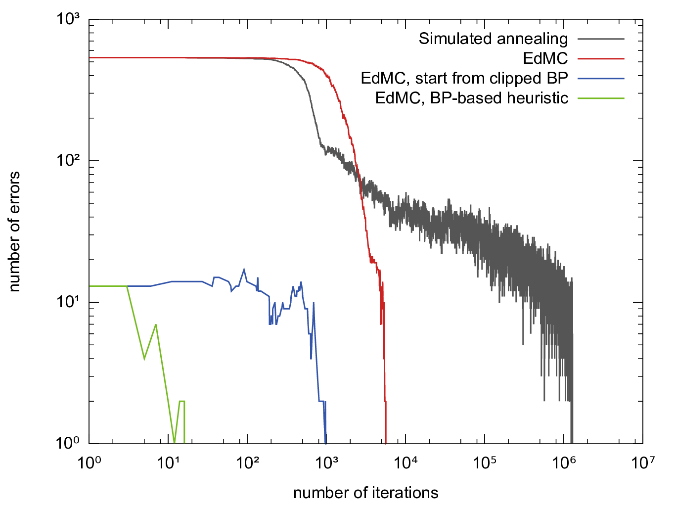
Fig. 5 shows the results of a test on one sample for $N=501$ , $\alpha=1.2$ , $L=4$ , $f=0.1$ . Although the search space is considerably larger, the behavior of the algorithm is very similar to what was observed in [8] for the binary, balanced and unbiased case: while EdMC reaches $0$ errors in a few iterations, standard SA plateaus and only eventually finds a solution, in several orders of magnitude more iterations (as is typical for these glassy systems, the time during which SA is trapped in a plateau increases exponentially with $N$ ). The heuristic enhancements further improve EdMC performance.

More specifically in this test all the variants of the EdMC were run at $y=\infty$ ; when the initial configuration was chosen at random, we started with external fields of low intensity $\gamma=0.5$ and progressively increased it by $\Delta\gamma=1.0$ after each greedy optimization procedure, thus avoiding inconsistencies in the messages and guaranteeing the convergence of BP even in the early stages, when the reference configuration $\tilde{W}$ is very far away from any solution. When starting from the clipped BP marginals the fields could be set directly at $\gamma=3.5$ .

On the other hand in the SA we observed that the chosen $\alpha$ was large enough to trap the standard Monte Carlo even with very slow cooling rates, so we had to resort to a different definition of the energy function

E_{\Delta}\left(\tilde{W}\right)=\sum_{\mu}\left(-\left(2\sigma^{\mu}-1\right)\left(\sum_{i}\tilde{W}_{i}\xi_{i}^{\mu}-\theta N\right)\right)_{+}

(17)

where $\left(x\right)_{+}=x$ if $x>0$ , $0$ otherwise; i.e. this energy function measures the negative of the sum of the so-called stabilities. The annealing scheme was carried out adopting a cooling rate of $r_{y}=1.005$ , which is multiplied to $y$ after every $100$ accepted moves, starting from an inverse temperature of $y=1.0$ .

In both the EdMC and the SA the firing threshold $\theta$ was set to its optimal value, which was determined analytically via replica calculations.

VI Conclusions

In this work, we extended a large deviation analysis of the solution space of a single layer neural network from the purely binary and balanced case [14] to the general discrete case. Despite some technical challenges in solving the equations, the results clearly indicate that the general qualitative picture is unchanged with respect to the binary case. In particular, for all values of the parameters and regardless of the number of synaptic states, we observe the existence of two distinct phases: one in which most solutions are isolated and hard to find, but there exists a dense and accessible cluster of solutions whose presence can be directly or indirectly exploited by heuristic solvers (e.g. by the EdMC algorithm); one in which this dense cluster has broken apart. The transition point $\alpha_{U}$ between these two phases was greater than $0.9\alpha_{c}$ in all our tested settings, i.e. it is fairly close to the maximal theoretical capacity. Both $\alpha_{c}$ and $\alpha_{U}$ grow with the number of synaptic states; however, the increase becomes rapidly very slow after the first few states: if there is a cost (metabolic or hardware) associated to adding more states to the synapses, this analysis suggests that the overall benefit of doing so would rapidly vanish. In other words, synapses may only need few bits of precision, both in the sense that efficient learning is still possible (contrary to what previous analyses suggested) and in the sense that, increasing the precision, the marginal advantage in terms of capacity decreases quite rapidly.

Our main drive for performing this analysis was to make the model more biologically plausible with respect to the binary case, while still keeping it simple enough so that the theoretical analysis can be performed (albeit with great difficulty, for computational and numerical reasons). Indeed, as we already mentioned, our model neurons are very crude simplifications of biological neurons; also, using uncorrelated inputs and outputs is hardly realistic, or at the very least there certainly are settings in which we would rather consider some kind of correlations. Despite these shortcomings, we believe that this analysis, together with the previous one for the binary case, bears a rather clear general message, namely that the qualitative picture is the same regardless of the finer detail. In particular, this picture was not affected in our analysis by any of the parameters (number of synaptic states, sparsity of the patterns). Also, we had already shown for the binary case that numerical tests performed on a handwritten-digit image-recognition benchmark indicate that even when using more “natural” (highly correlated and structured) patterns the heuristic learning algorithms invariably end up in a dense region of solutions such as those described by the theoretical analysis of the uncorrelated-inputs case.

Therefore, despite the inevitable shortcomings of the model, this analysis provides a plausible picture in which to frame the study of the synaptic precision of biological neurons in relation to their computational and representational power. In a nutshell, it suggests that low precision synapses are convenient for concrete implementations because the solution space has regions that can be exploited for learning efficiently, consistently with experimental biological results. Indeed, the learning mechanism must be different from what is usually employed in machine learning applications (stochastic gradient descent), but simple effective algorithms exist thanks to the peculiar structure of the solution space, with ample room for discretion in implementation details. This is clearly exemplified by the effectiveness of the Entropy-driven Monte Carlo technique that we introduced in [8] and that we extended here to the more general case. Establishing the presence of this geometrical picture in the learning of discrete deep forward networks and recurrent neural networks looks like a promising direction for future investigations.

Acknowledgements.

C.B., C.L. and R.Z. acknowledge the European Research Council for grant n° 267915.

Appendix A Franz-Parisi potential

In order to describe the geometrical properties of the solution space of the generalized perceptron, it is possible to carry out a mean-field analysis based on the computation of the Franz-Parisi potential. This method is conceptually divided in two stages: first we select a reference configuration $\tilde{W}$ from the equilibrium Boltzmann measure at a certain inverse temperature $\beta^{\prime}$ , then we evaluate the free energy of a coupled model where the configurations $\{W\}$ , at inverse temperature $\beta$ , are constrained to be exactly at a distance $D$ from the reference point:

\mathcal{S}_{FP}\left(\beta^{\prime},\beta,D\right)=\frac{1}{N}\left\langle\frac{1}{Z\left(\beta^{\prime}\right)}\sum_{\left\{\tilde{W}\right\}}e^{-\beta^{\prime}E\left(\tilde{W}\right)}\log\left(\sum_{\left\{W\right\}}e^{-\beta E\left(W\right)}\delta\left(d\left(W,\tilde{W}\right)-D\right)\right)\right\rangle_{\{\xi,\sigma\}}

(18)

Since we are interested in the constraint satisfaction problem, in our case both temperatures are set to zero ( $\beta,\beta^{\prime}\to\infty$ ). It is important to notice that the sampling of $\tilde{W}$ is not affected by the coupling, so it is extracted at random from a flat distribution over all possible solutions, and represents the typical case (i.e. numerically dominant in this measure).

The Franz-Parisi potential can thus be interpreted as a typical local entropy density:

\mathcal{S}_{FP}\left(D\right)=\frac{1}{N}\left\langle\left\langle\log\sum_{\left\{W\right\}}\mathbb{X}_{\xi,\sigma}\left(W\right)\delta\left(d\left(W,\tilde{W}\right)-D\right)\right\rangle_{\tilde{W}}\right\rangle_{\left\{\xi,\sigma\right\}}

(19)

with the definition of the indicator function $\mathbb{X}_{\xi,\sigma}\left(W\right)$ of equation 4 and the averaging $\left\langle\cdot\right\rangle_{\tilde{W}}$ is performed over the flat measure on all solutions to the problem.

It is possible to introduce a robustness parameter $K$ to stabilize the learned patterns (at the order $O\left(\sqrt{N}\right)$ ), so that each association is considered learned only if the output of the device is correct and the modulus of the activation $\left|\sum_{i=1}^{N}\frac{W_{i}\xi_{i}^{\mu}}{\sqrt{N}}-\theta\sqrt{N}\right|$ is above this threshold. The indicator function can be then redefined as:

\mathbb{X}_{\xi,\sigma}\left(W,K\right)=\prod_{\mu}\Theta\left(s^{\mu}\left(\sum_{i}\frac{W_{i}\xi_{i}^{\mu}}{\sqrt{N}}-\theta\sqrt{N}\right)-K\right)

(20)

where we omitted the indication of the ranges $i\in\left\{1,\dots,N\right\}$ and $\mu\in\left\{1,\dots,\alpha N\right\}$ for simplicity of notation, and we defined $s^{\mu}=2\sigma^{\mu}-1$ in order to convert between the device output $\sigma^{\mu}\in\left\{0,1\right\}$ and a more convenient representation $s^{\mu}\in\left\{-1,+1\right\}$ . Note that with this definition the average over the output $\sigma^{\mu}$ for any function $g\left(s^{\mu}\right)$ is defined as:

\left\langle g\left(s^{\mu}\right)\right\rangle_{s^{\mu}}=f^{\prime}g\left(1\right)+\left(1-f^{\prime}\right)g\left(-1\right)

(21)

i.e. we use the parameter $f^{\prime}$ to denote the output coding rate, which in principle can be distinguished from the input coding rate $f$ .

In order to perform the average over the measure of solutions $\tilde{W}$ and over the quenched disorder, we employ the replica trick: we introduce $\tilde{n}-1$ non interacting copies $\tilde{W}^{c}$ of the reference solution, and leave out the index $\tilde{W}^{c=1}$ for the replica appearing in the distance constraint. Furthermore we denote the $n$ replicas of the coupled solutions $W^{a}$ . Throughout this section, we will use the indices $a,b\in\left\{1,\dots,n\right\}$ for the replicated $W$ and $c,d\in\left\{1,\dots,\tilde{n}\right\}$ for the replicated $\tilde{W}$ , and we will omit the specification of the indices ranges in sums and products, for notational simplicity. In the end $\tilde{n}$ and $n$ will be sent to zero:

$\displaystyle\mathcal{S}_{FP}\left(D\right)$	$\displaystyle=$	$\displaystyle\frac{1}{N}\lim_{n,\tilde{n}\rightarrow 0}\frac{\partial}{\partial n}\left<\int\prod_{i,c}d\mu\left(\tilde{W}_{i}^{c}\right)\int\prod_{i,a}d\mu\left(W_{i}^{a}\right)\prod_{c}\mathbb{X}_{\xi,\sigma}\left(\tilde{W}^{c},K\right)\prod_{a}\mathbb{X}_{\xi,\sigma}\left(W^{a},K\right)\right.$	(22)
		$\displaystyle\qquad\qquad\qquad\left.\times\prod_{a}\delta\left(\frac{1}{2}\sum_{i}\left(W_{i}^{a}-\tilde{W}_{i}^{1}\right)^{2}-2DN\right)\right>_{\xi,\sigma}$
	$\displaystyle\equiv$	$\displaystyle\frac{1}{N}\lim_{n\rightarrow 0}\frac{\partial}{\partial n}\Omega_{FP}^{n}\left(D\right)$

where we used the definition of eq. (9) for the distance function $d\left(\cdot,\cdot\right)$ and introduced the measure over the possible values of the weights:

d\mu\left(W\right)=\sum_{l\in\mathcal{L}}\delta\left(W-l\right)

(23)

(In our experiments, we always used $\mathcal{L}=\left\{0,1,\dots,L\right\}$ , but the derivation is general.) In the last line of eq. (22) we also defined the replicated volume $\Omega_{FP}^{n}\left(D\right)$ .

As a first step we can introduce some auxiliary variables to substitute the arguments of the indicator functions:

	$\displaystyle\prod_{c}\mathbb{X}_{\xi,\sigma}\left(\tilde{W}^{c},K\right)\prod_{a}\mathbb{X}_{\xi,\sigma}\left(W^{a},K\right)=$		(24)
	$\displaystyle=\int\prod_{\mu,a}\frac{d\lambda_{\mu}^{a}d\hat{\lambda}_{\mu}^{a}}{2\pi}\int\prod_{\mu,c}\frac{d\tilde{\lambda}_{\mu}^{c}d\hat{\tilde{\lambda}}_{\mu}^{c}}{2\pi}\left\langle\prod_{\mu,a}\Theta\left(\sigma^{\mu}\lambda_{\mu}^{a}-K\right)\prod_{\mu,c}\Theta\left(\sigma^{\mu}\tilde{\lambda}_{\mu}^{c}-K\right)\right\rangle_{\sigma}\prod_{\mu,a}e^{i\lambda_{\mu}^{a}\hat{\lambda}_{\mu}^{a}}\prod_{\mu,c}e^{i\tilde{\lambda}_{\mu}^{c}\hat{\tilde{\lambda}}_{\mu}^{c}}\times$
	$\displaystyle\quad\times\prod_{\mu,i}\left(e^{i\theta\sqrt{N}\sum_{ac}\hat{\lambda}_{\mu}^{ca}}\left\langle\exp\left(-\frac{i}{\sqrt{N}}\left(\sum_{a}\hat{\lambda}_{\mu}^{a}W_{i}^{a}+\sum_{c}\hat{\tilde{\lambda}}_{\mu}^{c}\tilde{W}_{i}^{c}\right)\xi_{i}^{\mu}\right)\right\rangle_{\xi}\right)$

We can now perform the average over the pattern distribution $\left\langle\cdot\right\rangle_{\xi}=\int\prod_{i,\mu}\left(P\left(\xi_{i}^{\mu}\right)d\xi_{i}^{\mu}\right)$ :

	$\displaystyle\prod_{\mu,i}\left\langle\exp\left(-\frac{i}{\sqrt{N}}\left(\sum_{a}\hat{\lambda}_{\mu}^{a}W_{i}^{a}+\sum_{c}\hat{\tilde{\lambda}}_{\mu}^{c}\tilde{W}_{i}^{c}\right)\xi_{i}^{\mu}\right)\right\rangle_{\xi}=$		(25)
	$\displaystyle=\prod_{\mu}\exp\sum_{i}\log\left(1-\frac{i}{\sqrt{N}}\left(\sum_{a}\hat{\lambda}_{\mu}^{a}W_{i}^{a}+\sum_{c}\hat{\tilde{\lambda}}_{\mu}^{c}\tilde{W}_{i}^{c}\right)\overline{\xi}+\right.$
	$\displaystyle\qquad\left.-\frac{1}{2N}\left(\left(\sum_{a}\hat{\lambda}_{\mu}^{a}W_{i}^{a}\right)^{2}+\left(\sum_{c}\hat{\tilde{\lambda}}_{\mu}^{c}\tilde{W}_{i}^{c}\right)^{2}+2\sum_{ac}\hat{\lambda}_{\mu}^{a}\hat{\tilde{\lambda}}_{\mu}^{c}W_{i}^{a}\tilde{W}_{i}^{c}\right)\overline{\xi^{2}}\right)$
	$\displaystyle=\prod_{\mu}\exp\left(-i\overline{\xi}\sqrt{N}\left(\sum_{a}\hat{\lambda}_{\mu}^{a}\sum_{i}\frac{W_{i}^{a}}{N}+\sum_{c}\hat{\tilde{\lambda}}_{\mu}^{c}\sum_{i}\frac{W_{i}^{c}}{N}\right)+\right.$
	$\displaystyle\qquad\left.-\frac{\sigma_{\xi}^{2}}{2}\left(\sum_{ab}\hat{\lambda}_{\mu}^{a}\hat{\lambda}_{\mu}^{b}\sum_{i}\frac{W_{i}^{a}W_{i}^{b}}{N}+\sum_{cd}\hat{\lambda}_{\mu}^{c}\hat{\lambda}_{\mu}^{d}\sum_{i}\frac{\tilde{W}_{i}^{c}\tilde{W}_{i}^{d}}{N}+2\sum_{ac}\hat{\lambda}_{\mu}^{a}\hat{\tilde{\lambda}}_{\mu}^{c}\sum_{i}\frac{W_{i}^{a}\tilde{W}_{i}^{c}}{N}\right)\right)$

where $\overline{\xi}$ indicates the average of the inputs and $\sigma_{\xi}^{2}$ is their variance.

All the overlaps (such as $\frac{1}{N}\sum_{i}W_{i}^{a}W_{i}^{b}$ ) can now be replaced with order parameters via Dirac $\delta$ distributions. In the case of the generalized perceptron we also need to introduce two specific parameters for the $L^{1}$ -norm and for the $L^{2}$ -norm.

Maximum capacity with biased patterns can be achieved if the mean value of the synaptic weights $\overline{W}$ is on the threshold given by the ratio:

\displaystyle\overline{W}

\displaystyle=

\displaystyle\frac{\theta}{f}

(26)

and because of the unbalanced distribution of the outputs we also need to introduce an $O\left(\frac{1}{\sqrt{N}}\right)$ correction controlled by the order parameter $M$ :

\displaystyle\sum_{i}\frac{W_{i}}{N}

\displaystyle=

\displaystyle\overline{W}+\frac{M}{\sqrt{N}}

(27)

We can define the following:

•

$\sum_{i}\frac{\left(W_{i}^{a}\right)^{2}}{N}=Q^{a}$ , $\sum_{i}\frac{\left(\tilde{W}_{i}^{c}\right)^{2}}{N}=\tilde{Q^{c}}$
•

$\sum_{i}\frac{W_{i}^{a}}{N}=\overline{W}+\frac{M^{a}}{\sqrt{N}}$ , $\sum_{i}\frac{\tilde{W}_{i}^{c}}{N}=\overline{\tilde{W}}+\frac{\tilde{M}^{c}}{\sqrt{N}}$
•

$\sum_{i}\frac{W_{i}^{a}W_{i}^{b}}{N}=q^{ab}$ , $\sum_{i}\frac{\tilde{W}_{i}^{c}\tilde{W}_{i}^{d}}{N}=\tilde{q}^{cd}$ , $\sum_{i}\frac{W_{i}^{a}\tilde{W}_{i}^{c}}{N}=S^{ca}$

After these substitutions in the expression of the replicated volume $\Omega^{n}\left(D\right)$ , we use the integral representation of the Dirac $\delta$ distributions, introducing the required conjugate parameters, and rearrange the integrals so that it becomes possible to factorize over the $\mu$ and $i$ indices:

$\displaystyle\Omega_{FP}^{n}\left(D\right)$	$\displaystyle=$	$\displaystyle\lim_{\tilde{n}\rightarrow 0}\int\prod_{c>d}\frac{d\tilde{q}^{cd}d\hat{\tilde{q}}^{cd}}{\left(2\pi/N\right)}\int\prod_{a>b}\frac{dq^{ab}d\hat{q}^{ab}}{\left(2\pi/N\right)}\int\prod_{c}\frac{d\tilde{Q}^{c}d\hat{\tilde{Q}}^{c}}{\left(2\pi/N\right)}\int\prod_{a}\frac{dQ^{a}d\hat{Q}^{a}}{\left(2\pi/N\right)}$	(28)
		$\displaystyle\qquad\int\prod_{c}\frac{d\tilde{M}^{c}d\hat{\tilde{M}}^{c}}{\left(2\pi/\sqrt{N}\right)}\int\prod_{a}\frac{dM^{a}d\hat{M}^{a}}{\left(2\pi/\sqrt{N}\right)}\int\prod_{ca}\frac{dS^{ca}d\hat{S}^{ca}}{\left(2\pi/N\right)}$
		$\displaystyle\qquad\int\prod_{a}\frac{d\hat{D}^{a}}{2\pi}G_{1}\,\left(G_{S}\right)^{N}\,\left(G_{E}\right)^{\alpha N}$

where we have singled out a first term $G_{1}$ and the so-called entropic and energetic contributions $G_{S}$ , $G_{E}$ :

$\displaystyle G_{1}$	$\displaystyle=$	$\displaystyle\exp\left(-N\left(\sum_{c>d}\hat{\tilde{q}}^{cd}\tilde{q}^{cd}+\sum_{a>b}\hat{q}^{ab}q^{ab}+\sum_{c}\hat{\tilde{Q}}^{c}\tilde{Q}^{c}+\sum_{a}\hat{Q}^{a}Q^{a}+\sum_{c}\hat{\tilde{M}}^{c}\left(\frac{\tilde{M}^{c}}{\sqrt{N}}+\overline{\tilde{W}}\right)+\right.\right.$	(29)
		$\displaystyle\left.\left.+\sum_{a}\hat{M}^{a}\left(\frac{M^{a}}{\sqrt{N}}+\overline{W}\right)+\sum_{ca}\hat{S}^{ca}S^{ca}+\sum_{a}\hat{D}^{a}\left(\frac{1}{2}Q^{a}+\frac{1}{2}\tilde{Q}^{1}-S^{1a}-2D\right)\right)\right)$	(29)
$\displaystyle G_{S}$	$\displaystyle=$	$\displaystyle\int\prod_{c}d\mu\left(\tilde{W}^{c}\right)\int\prod_{a}d\mu\left(W^{a}\right)\exp\left(\sum_{c>d}\hat{\tilde{q}}^{cd}\tilde{W}^{c}\tilde{W}^{d}+\sum_{a>b}\hat{q}^{ab}W^{a}W^{b}+\right.$	(30)
		$\displaystyle\left.+\sum_{c}\hat{\tilde{Q}}^{c}\left(\tilde{W}^{c}\right)^{2}+\sum_{a}\hat{Q}^{a}\left(W^{a}\right)^{2}+\sum_{c}\hat{\tilde{M}}^{c}\tilde{W}^{c}+\sum_{a}\hat{M}^{a}W^{a}+\sum_{ca}\hat{S}^{ca}W^{a}\tilde{W}^{c}\right)$	(30)
$\displaystyle G_{E}$	$\displaystyle=$	$\displaystyle\int\prod_{a}\frac{d\lambda^{a}d\hat{\lambda}^{a}}{2\pi}\int\prod_{c}\frac{d\tilde{\lambda}^{c}d\hat{\tilde{\lambda}}^{c}}{2\pi}\left\langle\prod_{a}\Theta\left(s\lambda^{a}-K\right)\prod_{c}\Theta\left(s\tilde{\lambda}^{c}-K\right)\right\rangle_{s}\times$	(31)
		$\displaystyle\times\exp\left(i\left(\sum_{a}\lambda^{a}\hat{\lambda}^{a}+\sum_{c}\tilde{\lambda}^{c}\hat{\tilde{\lambda}}^{c}-\overline{\xi}\sum_{a}\hat{\lambda}^{a}M^{a}-\overline{\xi}\sum_{c}\hat{\tilde{\lambda}}^{c}\tilde{M}^{c}\right)+\right.$
		$\displaystyle\left.\quad-\frac{1}{2}\sigma_{\xi}^{2}\sum_{a}\left(\hat{\lambda}^{a}\right)^{2}Q^{a}-\frac{1}{2}\sigma_{\xi}^{2}\sum_{c}\left(\hat{\tilde{\lambda}}^{c}\right)^{2}\tilde{Q}^{c}-\frac{1}{2}\sigma_{\xi}^{2}\sum_{(a,b)}\hat{\lambda}^{a}\hat{\lambda}^{b}q^{ab}-\frac{1}{2}\sigma_{\xi}^{2}\sum_{(c,d)}\hat{\tilde{\lambda}}^{c}\hat{\tilde{\lambda}}^{d}\tilde{q}^{cd}-\sigma_{\xi}^{2}\sum_{ac}\hat{\lambda}^{a}\hat{\tilde{\lambda}}^{c}S^{ac}\right)$

Note that we dropped the indices $i$ and $\mu$ from all quantities since we have rearranged the terms and factorized the contributions; in particular, note that the indices were dropped from the weights $W^{a}$ , $\tilde{W}^{c}$ and the output $s$ .

A.1 Replica Symmetric Ansatz

To proceed with the calculations we now have to make an assumption on the structure of the replicated order parameters, the simplest possible one being the symmetric Ansatz, where one can drop all the dependencies on the replica indices. We only have to make a distinction between the overlaps $S$ and $\tilde{S}$ , since the first one enters also in the expression of the constraint on the distance $d\left(W,\tilde{W}\right)$ :

•

$S^{ca}=S$ for $c=1$ , $S^{ca}=\tilde{S}$ for $c\neq 1$
•

$Q^{a}=Q$ , $\tilde{Q}^{c}=\tilde{Q}$ , $M^{a}=M$ , $\tilde{M}^{c}=\tilde{M}$ , $q^{ab}=q$ , $\tilde{q}^{cd}=\tilde{q}$ , $\hat{D}^{ca}=\hat{D}$ .

The first term $G_{1}$ of the expression of the volume can now be simplified, and the $\tilde{n}\to 0$ can be taken, obtaining:

$\displaystyle G_{1}$	$\displaystyle=\lim_{\tilde{n}\rightarrow 0}\exp\left(-N\left(\frac{\tilde{n}\left(\tilde{n}-1\right)}{2}\hat{\tilde{q}}\tilde{q}+\frac{n\left(n-1\right)}{2}\hat{q}q+\tilde{n}\hat{\tilde{Q}}\tilde{Q}+n\hat{Q}Q+\right.\right.$	(32)
	$\displaystyle\left.\left.\qquad+\tilde{n}\hat{\tilde{M}}\overline{\tilde{W}}+n\hat{M}\overline{W}+n\hat{S}S-\left(1-\tilde{n}\right)n\hat{\tilde{S}}\tilde{S}+n\hat{D}\left(\frac{1}{2}Q+\frac{1}{2}\tilde{Q}-S-2D\right)\right)\right)$
	$\displaystyle=\exp\left(-Nn\left(-\frac{1}{2}\hat{q}q+\hat{Q}Q+\hat{M}\overline{W}+\hat{S}S-\hat{\tilde{S}}\tilde{S}+\hat{D}\left(\frac{1}{2}Q+\frac{1}{2}\tilde{Q}-S-2D\right)\right)\right)$

After the substitution of the RS Ansatz, the entropic term reads:

$\displaystyle G_{S}$	$\displaystyle=$	$\displaystyle\int\prod_{c}d\mu\left(\tilde{W}^{c}\right)\int\prod_{a}d\mu\left(W^{a}\right)\exp\left(\left(\hat{\tilde{Q}}-\frac{1}{2}\hat{\tilde{q}}\right)\sum_{c}\left(\tilde{W}^{c}\right)^{2}+\left(\hat{Q}-\frac{1}{2}\hat{q}\right)\sum_{a}\left(W^{a}\right)^{2}+\right.$	(33)
		$\displaystyle+\frac{1}{2}\hat{\tilde{q}}\left(\sum_{c}\tilde{W}^{c}\right)^{2}+\frac{1}{2}\hat{q}\left(\sum_{a}W^{a}\right)^{2}+\hat{\tilde{M}}\sum_{c}\tilde{W}^{c}+\hat{M}\sum_{a}W^{a}+$
		$\displaystyle\left.+\left(\hat{S}-\hat{\tilde{S}}\right)\sum_{a}W^{a}\tilde{W}^{1}+\hat{\tilde{S}}\sum_{a}W^{a}\sum_{c}\tilde{W}^{c}\right)$

Now, in order to be able to factorize over the replica index $c$ , we need to write:

\hat{\tilde{S}}\sum_{a}W^{a}\sum_{c}\tilde{W}^{c}=\frac{1}{2}\hat{\tilde{S}}\left(\sum_{a}W^{a}+\sum_{c}\tilde{W}^{c}\right)^{2}-\frac{1}{2}\hat{\tilde{S}}\left(\sum_{a}W^{a}\right)^{2}-\frac{1}{2}\hat{\tilde{S}}\left(\sum_{c}\tilde{W}^{c}\right)^{2}

and then we perform some Hubbard-Stratonovich transformations, introducing the variables $x$ , $z$ and $\tilde{z}$ .

Using the usual notation $\int\mathcal{D}z=\int_{-\infty}^{+\infty}\frac{dz}{\sqrt{2\pi}}e^{-\frac{z^{2}}{2}}$ for Gaussian integrals, we get:

$\displaystyle G_{S}$	$\displaystyle=$	$\displaystyle\int\mathcal{D}x\int\mathcal{D}z\int\mathcal{D}\tilde{z}$	(34)
		$\displaystyle\int\prod_{c}d\mu\left(\tilde{W}^{c}\right)\exp\left(\left(\hat{\tilde{Q}}-\frac{1}{2}\hat{\tilde{q}}\right)\sum_{c}\left(\tilde{W}^{c}\right)^{2}+\left(\tilde{z}\sqrt{\hat{\tilde{q}}-\hat{\tilde{S}}}+x\sqrt{\hat{\tilde{S}}}+\hat{\tilde{M}}\right)\sum_{c}\tilde{W}^{c}\right)\times$
		$\displaystyle\times\int\prod_{a}d\mu\left(W^{a}\right)\exp\left(\left(\hat{Q}-\frac{1}{2}\hat{q}\right)\sum_{a}\left(W^{a}\right)^{2}+\left(z\sqrt{\hat{q}-\hat{\tilde{S}}}+x\sqrt{\hat{\tilde{S}}}+\hat{M}+\left(\hat{S}-\hat{\tilde{S}}\right)\tilde{W}^{1}\right)\sum_{a}W^{a}\right)$

Since the expression is now factorized, with the definitions:

$\displaystyle\tilde{A}\left(\tilde{W},\tilde{z},x\right)$	$\displaystyle=$	$\displaystyle\left(\hat{\tilde{Q}}-\frac{1}{2}\hat{\tilde{q}}\right)\tilde{W}^{2}+\left(\tilde{z}\sqrt{\hat{\tilde{q}}-\hat{\tilde{S}}}+x\sqrt{\hat{\tilde{S}}}+\tilde{M}\right)\tilde{W}$	(35)
$\displaystyle A\left(W,\tilde{W},z,x\right)$	$\displaystyle=$	$\displaystyle\left(\hat{Q}-\frac{1}{2}\hat{q}\right)W^{2}+\left(z\sqrt{\hat{q}-\hat{\tilde{S}}}+x\sqrt{\hat{\tilde{S}}}+\hat{M}+\Delta\hat{S}\tilde{W}\right)W$	(36)
$\displaystyle\Delta\hat{S}$	$\displaystyle=$	$\displaystyle\hat{S}-\hat{\tilde{S}}$	(37)

we can first take the limit $\tilde{n}\to 0$ , restoring the presence of the denominator:

\displaystyle G_{S}

\displaystyle=

\displaystyle\int\mathcal{D}x\int\mathcal{D}z\int\mathcal{D}\tilde{z}\frac{\int d\mu\left(\tilde{W}\right)\exp\left(\tilde{A}\left(\tilde{W},\tilde{z},x\right)\right)\int\prod_{a}d\mu\left(W^{a}\right)\prod_{a}\exp\left(A^{a}\left(W^{a},\tilde{W},z,x\right)\right)}{\int d\mu\left(\tilde{W}\right)\exp\left(\tilde{A}\left(\tilde{W},\tilde{z},x\right)\right)}

(38)

And then, in the limit $n\to 0$ , we can write:

\displaystyle\mathcal{G}_{S}=\frac{1}{n}\log G_{S}

\displaystyle=

\displaystyle\int\mathcal{D}x\int\mathcal{D}z\int\mathcal{D}\tilde{z}\frac{\int d\mu\left(\tilde{W}\right)\exp\left(\tilde{A}\left(\tilde{W},\tilde{z},x\right)\right)\log\left(\int d\mu\left(W\right)\exp\left(A\left(W,\tilde{W},z,x\right)\right)\right)}{\int d\mu\left(\tilde{W}\right)\exp\left(\tilde{A}\left(\tilde{W},\tilde{z},x\right)\right)}

(39)

Then we perform two rotations between the integration variables ( $\tilde{z}$ , $x$ ) and ( $z$ , $x$ ), in order to compute analytically the $\int\mathcal{D}x$ integral, obtaining:

	$\displaystyle\mathcal{G}_{S}=$		(40)
	$\displaystyle\int\negthickspace\mathcal{D}z\int\negthickspace\mathcal{D}\tilde{z}\frac{\sum_{\tilde{l}}\exp\left(\left(\hat{\tilde{Q}}-\frac{1}{2}\hat{\tilde{q}}\right)\tilde{l}^{2}+\left(\hat{\tilde{M}}+\tilde{z}\sqrt{\hat{q}}\right)\tilde{l}\right)\log\left(\sum_{l}\exp\left(\left(\hat{Q}-\frac{1}{2}\hat{q}\right)l^{2}+\left(\hat{M}+z\sqrt{\frac{\hat{q}\hat{\tilde{q}}-\hat{\tilde{S}}^{2}}{\hat{\tilde{q}}}}+\tilde{z}\frac{\hat{\tilde{S}}}{\sqrt{\hat{\tilde{q}}}}+\Delta\hat{S}\,\,\tilde{l}\right)l\right)\right)}{\sum_{\tilde{l}}\exp\left(\left(\hat{\tilde{Q}}-\frac{1}{2}\hat{\tilde{q}}\right)\tilde{l}^{2}+\left(\hat{\tilde{M}}+\tilde{z}\sqrt{\hat{q}}\right)\tilde{l}\right)}$

We proceed in a similar way with the computation of the energetic term:

$\displaystyle G_{E}$	$\displaystyle=$	$\displaystyle\int\mathcal{D}x\int\prod_{a}\frac{d\lambda^{a}d\hat{\lambda}^{a}}{2\pi}\int\prod_{c}\frac{d\tilde{\lambda}^{c}d\hat{\tilde{\lambda}}^{c}}{2\pi}\left\langle\prod_{a}\Theta\left(s\lambda^{a}-K\right)\prod_{c}\Theta\left(s\tilde{\lambda}^{c}-K\right)\right\rangle_{s}\times$	(41)
		$\displaystyle\times\exp\left(i\sum_{a}\hat{\lambda}^{a}\left(\lambda^{a}-\overline{\xi}M-x\sqrt{\sigma_{\xi}^{2}\tilde{S}}\right)+i\sum_{c}\hat{\tilde{\lambda}}^{c}\left(\tilde{\lambda}^{c}-\overline{\xi}\tilde{M}-x\sqrt{\sigma_{\xi}^{2}\tilde{S}}\right)-\frac{1}{2}\sigma_{\xi}^{2}\left(Q-q\right)\sum_{a}\left(\hat{\lambda}^{a}\right)^{2}+\right.$
		$\displaystyle\left.-\frac{1}{2}\sigma_{\xi}^{2}\left(\tilde{Q}-\tilde{q}\right)\sum_{c}\left(\hat{\tilde{\lambda}}^{c}\right)^{2}-\frac{1}{2}\sigma_{\xi}^{2}\left(q-\tilde{S}\right)\left(\sum_{a}\hat{\lambda}^{a}\right)^{2}-\frac{1}{2}\sigma_{\xi}^{2}\left(\tilde{q}-\tilde{S}\right)\left(\sum_{c}\hat{\tilde{\lambda}}^{c}\right)^{2}-\sigma_{\xi}^{2}\left(S-\tilde{S}\right)\hat{\tilde{\lambda}}^{1}\sum_{a}\hat{\lambda}^{a}\right)$

We define:

	$\displaystyle\tilde{B}\left(\tilde{\lambda},\tilde{z},x\right)$	$\displaystyle=$	$\displaystyle-\frac{1}{2}\sigma_{\xi}^{2}\left(\tilde{Q}-\tilde{q}\right)\hat{\tilde{\lambda}}^{2}+i\left(\tilde{\lambda}-\overline{\xi}\tilde{M}-x\sqrt{\sigma_{\xi}^{2}\tilde{S}}-\tilde{z}\sqrt{\sigma_{\xi}^{2}\left(\tilde{q}-\tilde{S}\right)}\right)\hat{\tilde{\lambda}}$		(42)
	$\displaystyle B\left(\lambda,\tilde{\lambda},z,x\right)$	$\displaystyle=$	$\displaystyle-\frac{1}{2}\sigma_{\xi}^{2}\left(Q-q\right)\hat{\lambda}^{2}+i\left(\lambda-\overline{\xi}M-x\sqrt{\sigma_{\xi}^{2}\tilde{S}}-z\sqrt{\sigma_{\xi}^{2}\left(q-\tilde{S}\right)}+i\sigma_{\xi}^{2}\left(S-\tilde{S}\right)\hat{\tilde{\lambda}}\right)\hat{\lambda}$		(43)

and in the $n\to 0$ limit we find:

	$\displaystyle\mathcal{G}_{E}=\frac{1}{n}\log G_{E}=$		(44)
	$\displaystyle\int\mathcal{D}x\int\mathcal{D}z\int\mathcal{D}\tilde{z}\left\langle\frac{\int\frac{d\tilde{\lambda}d\hat{\tilde{\lambda}}}{2\pi}\Theta\left(s\tilde{\lambda}-K\right)\exp\left(\tilde{B}\left(\tilde{\lambda},\tilde{z},x\right)\right)\log\left(\int\frac{d\lambda d\hat{\lambda}}{2\pi}\Theta\left(s\lambda-K\right)\exp\left(B\left(\lambda,\tilde{\lambda},z,x\right)\right)\right)}{\int\frac{d\tilde{\lambda}d\hat{\tilde{\lambda}}}{2\pi}\Theta\left(s\tilde{\lambda}-K\right)\exp\left(\tilde{B}\left(\tilde{\lambda},\tilde{z},x\right)\right)}\right\rangle_{s}$

We leave the output average written implicitly (see eq. (21)) for simplicity. We can evaluate the $\hat{\lambda}$ and $\lambda$ integrals introducing the normalized integral function:

\displaystyle H\left(x\right)

\displaystyle=\int_{x}^{\infty}\mathcal{D}x=

\displaystyle\frac{1}{2}\erfc\left(\frac{x}{\sqrt{2}}\right)

(45)

Performing the change of variables $z^{\prime}=z-i\hat{\tilde{\lambda}}\frac{\Delta S\sqrt{\sigma_{\xi}^{2}}}{\sqrt{q-\tilde{S}}}$ , where we set $\Delta S=S-\tilde{S}$ , and two rotations between ( $\tilde{z}$ , $x$ ) and ( $z$ , $x$ ) one can isolate the dependence over $x$ and compute the $\int\mathcal{D}x$ integral analytically:

	$\displaystyle\int\mathcal{D}x\,H\left(\frac{K-\overline{\xi}\tilde{M}-\tilde{z}\sqrt{\sigma_{\xi}^{2}\tilde{q}}-z\left(\frac{\Delta S\sqrt{\sigma_{\xi}^{2}\tilde{q}}}{\sqrt{q\tilde{q}-\tilde{S}^{2}}}\right)-x\left(\frac{\Delta S\sqrt{\sigma_{\xi}^{2}\left(\tilde{q}-\tilde{S}\right)\tilde{S}}}{\sqrt{\left(q\tilde{q}-\tilde{S}^{2}\right)\left(q-\tilde{S}\right)}}\right)}{\sqrt{\sigma_{\xi}^{2}\left(\tilde{Q}-\tilde{q}-\frac{\left(\Delta S\right)^{2}}{q-\tilde{S}}\right)}}\right)=$
	$\displaystyle=H\left(\frac{K-\overline{\xi}\tilde{M}-\tilde{z}\sqrt{\sigma_{\xi}^{2}\tilde{q}}-z\left(\frac{\Delta S\sqrt{\sigma_{\xi}^{2}\tilde{q}}}{\sqrt{q\tilde{q}-\tilde{S}^{2}}}\right)}{\sqrt{\sigma_{\xi}^{2}\left(\tilde{Q}-\tilde{q}-\frac{\left(\Delta S\right)^{2}}{q-\tilde{S}}+\frac{\Delta S^{2}\tilde{S}\left(\tilde{q}-\tilde{S}\right)}{\left(q\tilde{q}-\tilde{S}^{2}\right)\left(q-\tilde{S}\right)}\right)}}\right)$

now we can integrate over $\hat{\tilde{\lambda}}$ and $\tilde{\lambda}$ to obtain:

	$\displaystyle\mathcal{G}_{E}=$		(46)
	$\displaystyle=\left\langle\int\mathcal{D}z\int\mathcal{D}\tilde{z}\frac{H\left(\frac{K-s\overline{\xi}\tilde{M}-\tilde{z}\sqrt{\sigma_{\xi}^{2}\tilde{q}}-z\left(\frac{\Delta S\sqrt{\sigma_{\xi}^{2}\tilde{q}}}{\sqrt{q\tilde{q}-\tilde{S}^{2}}}\right)}{\sqrt{\sigma_{\xi}^{2}\left(\tilde{Q}-\tilde{q}-\frac{\left(\Delta S\right)^{2}}{q-\tilde{S}}+\frac{\Delta S^{2}\tilde{S}\left(\tilde{q}-\tilde{S}\right)}{\left(q\tilde{q}-\tilde{S}^{2}\right)\left(q-\tilde{S}\right)}\right)}}\right)\log\left(H\left(\frac{K-s\overline{\xi}M-z\sqrt{\sigma_{\xi}^{2}\left(\frac{q\tilde{q}-\tilde{S}^{2}}{\tilde{q}}\right)}-\tilde{z}\sqrt{\sigma_{\xi}^{2}\frac{\tilde{S}^{2}}{\tilde{q}}}}{\sqrt{\sigma_{\xi}^{2}\left(Q-q\right)}}\right)\right)}{H\left(\frac{K-s\overline{\xi}\tilde{M}-\tilde{z}\sqrt{\sigma_{\xi}^{2}\tilde{q}}}{\sqrt{\sigma_{\xi}^{2}\left(\tilde{Q}-\tilde{q}\right)}}\right)}\right\rangle_{s}$

Plugging all the terms into the expression of the volume, we can now write a saddle point approximation for the local entropy $\Phi\left(D\right)$ :

	$\displaystyle\mathcal{S}_{FP}\left(D\right)\,\,\,\,\text{$\approx$}\,\,\,\,\frac{1}{2}\hat{q}q-\hat{Q}Q-\hat{M}\overline{W}-\hat{S}S+\hat{\tilde{S}}\tilde{S}-\hat{D}\left(\frac{1}{2}Q+\frac{1}{2}\tilde{Q}-S-2D\right)+$		(47)
	$\displaystyle+\int\mathcal{D}z\int\mathcal{D}\tilde{z}\frac{\sum_{\tilde{l}}\exp\left(\left(\hat{\tilde{Q}}-\frac{1}{2}\hat{\tilde{q}}\right)\tilde{l}^{2}+\left(\hat{\tilde{M}}+\tilde{z}\sqrt{\hat{q}}\right)\tilde{l}\right)\log\left(\sum_{l}\exp\left(\left(\hat{Q}-\frac{1}{2}\hat{q}\right)l^{2}+\left(\hat{M}+z\sqrt{\frac{\hat{q}\hat{\tilde{q}}-\hat{\tilde{S}}^{2}}{\hat{\tilde{q}}}}+\tilde{z}\frac{\hat{\tilde{S}}}{\sqrt{\hat{\tilde{q}}}}+\Delta\hat{S}\,\,\tilde{l}\right)l\right)\right)}{\sum_{\tilde{l}}\exp\left(\left(\hat{\tilde{Q}}-\frac{1}{2}\hat{\tilde{q}}\right)\tilde{l}^{2}+\left(\hat{\tilde{M}}+\tilde{z}\sqrt{\hat{q}}\right)\tilde{l}\right)}+$
	$\displaystyle+\alpha\left\langle\int\mathcal{D}z\int\mathcal{D}\tilde{z}\frac{H\left(\frac{K-s\overline{\xi}\tilde{M}-\tilde{z}\sqrt{\sigma_{\xi}^{2}\tilde{q}}-z\left(\frac{\Delta S\sqrt{\sigma_{\xi}^{2}\tilde{q}}}{\sqrt{q\tilde{q}-\tilde{S}^{2}}}\right)}{\sqrt{\sigma_{\xi}^{2}\left(\tilde{Q}-\tilde{q}-\frac{\left(\Delta S\right)^{2}}{q-\tilde{S}}+\frac{\Delta S^{2}\tilde{S}\left(\tilde{q}-\tilde{S}\right)}{\left(q\tilde{q}-\tilde{S}^{2}\right)\left(q-\tilde{S}\right)}\right)}}\right)\log\left(H\left(\frac{K-s\overline{\xi}M-z\sqrt{\sigma_{\xi}^{2}\left(\frac{q\tilde{q}-\tilde{S}^{2}}{\tilde{q}}\right)}-\tilde{z}\sqrt{\sigma_{\xi}^{2}\frac{\tilde{S}^{2}}{\tilde{q}}}}{\sqrt{\sigma_{\xi}^{2}\left(Q-q\right)}}\right)\right)}{H\left(\frac{K-s\overline{\xi}\tilde{M}-\tilde{z}\sqrt{\sigma_{\xi}^{2}\tilde{q}}}{\sqrt{\sigma_{\xi}^{2}\left(\tilde{Q}-\tilde{q}\right)}}\right)}\right\rangle_{s}$

where all the order parameters must satisfy the saddle point equations, found by requiring the stationarity condition $\delta\mathcal{S}_{FP}=0$ :

	$\displaystyle q=-2\frac{\partial}{\partial\hat{q}}\mathcal{G}_{S};\quad Q=\frac{\partial}{\partial\hat{Q}}\mathcal{G}_{S};\quad\overline{W}=\frac{\partial}{\partial\hat{M}}\mathcal{G}_{S};\quad\tilde{S}=\frac{\partial}{\partial\hat{\tilde{S}}}\mathcal{G}_{S};\quad S=\frac{Q}{2}+\frac{\tilde{Q}}{2}-2D;\quad 0=\frac{\partial}{\partial\hat{S}}\mathcal{G}_{S}-S;$		(48)
	$\displaystyle\hat{q}=-2\alpha\frac{\partial}{\partial q}\mathcal{G}_{E};\quad\hat{Q}=-\frac{\hat{D}}{2}+\alpha\frac{\partial}{\partial Q}\mathcal{G}_{E};\quad\hat{D}=\hat{S}-\alpha\frac{\partial}{\partial S}\mathcal{G}_{E};\quad\hat{\tilde{S}}=-\alpha\frac{\partial}{\partial\tilde{S}}\mathcal{G}_{E};\quad\hat{M}=0;\quad 0=\frac{\partial}{\partial M}\mathcal{G}_{E}.$

Since the reference solution is sampled independently from the flat Boltzmann distribution, the typical value for the order parameters $\tilde{Q}$ , $\tilde{q}$ , and $\tilde{M}$ can be determined by studying the simpler uncoupled replicated system:

\displaystyle\tilde{\Omega}^{n}

\displaystyle=

\displaystyle\left\langle\int\prod_{i,c}d\mu\left(\tilde{W}_{i}^{c}\right)\prod_{c}\mathbb{X}_{\xi,\sigma}\left(\tilde{W}^{c},K\right)\right\rangle_{\xi,\sigma}

In the end one can explicitly use the measure on the weights (eq. (23)) and get the saddle point equations:

$\displaystyle\tilde{q}$	$\displaystyle=$	$\displaystyle\int\mathcal{D}\tilde{z}\frac{\sum_{\tilde{l}}\left(\left(\tilde{l}^{2}-\frac{\tilde{l}\tilde{z}}{\sqrt{\hat{\tilde{q}}}}\right)\exp\left(\left(\hat{\tilde{Q}}-\frac{1}{2}\hat{\tilde{q}}\right)\tilde{l}^{2}+\left(\tilde{z}\sqrt{\hat{\tilde{q}}}\right)\tilde{l}\right)\right)}{\sum_{\tilde{l}}\exp\left(\left(\hat{\tilde{Q}}-\frac{1}{2}\hat{\tilde{q}}\right)\tilde{l}^{2}+\left(\tilde{z}\sqrt{\hat{\tilde{q}}}\right)\tilde{l}\right)}$	(49)
$\displaystyle\tilde{Q}$	$\displaystyle=$	$\displaystyle\int\mathcal{D}\tilde{z}\frac{\sum_{\tilde{l}}\left(\tilde{l}^{2}\exp\left(\left(\hat{\tilde{Q}}-\frac{1}{2}\hat{\tilde{q}}\right)\tilde{l}^{2}+\left(\tilde{z}\sqrt{\hat{\tilde{q}}}\right)\tilde{l}\right)\right)}{\sum_{\tilde{l}}\exp\left(\left(\hat{\tilde{Q}}-\frac{1}{2}\hat{\tilde{q}}\right)\tilde{l}^{2}+\left(\tilde{z}\sqrt{\hat{\tilde{q}}}\right)\tilde{l}\right)}$	(50)
$\displaystyle\overline{\tilde{W}}$	$\displaystyle=$	$\displaystyle\int\mathcal{D}\tilde{z}\frac{\sum_{\tilde{l}}\left(\tilde{l}\exp\left(\left(\hat{\tilde{Q}}-\frac{1}{2}\hat{\tilde{q}}\right)\tilde{l}^{2}+\left(\tilde{z}\sqrt{\hat{\tilde{q}}}\right)\tilde{l}\right)\right)}{\sum_{\tilde{l}}\exp\left(\left(\hat{\tilde{Q}}-\frac{1}{2}\hat{\tilde{q}}\right)\tilde{l}^{2}+\left(\tilde{z}\sqrt{\hat{\tilde{q}}}\right)\tilde{l}\right)}$	(51)
$\displaystyle 0$	$\displaystyle=$	$\displaystyle\left\langle\int\mathcal{D}\tilde{z}\,\mathcal{G}\left(\frac{K-s\overline{\xi}\tilde{M}-\tilde{z}\sqrt{\sigma_{\xi}^{2}\tilde{q}}}{\sqrt{\sigma_{\xi}^{2}\left(\tilde{Q}-\tilde{q}\right)}}\right)\right\rangle_{s}$	(52)
$\displaystyle\hat{\tilde{q}}$	$\displaystyle=$	$\displaystyle\alpha\left\langle\int\mathcal{D}\tilde{z}\,\mathcal{G}\left(\frac{K-s\overline{\xi}\tilde{M}-\tilde{z}\sqrt{\sigma_{\xi}^{2}\tilde{q}}}{\sqrt{\sigma_{\xi}^{2}\left(\tilde{Q}-\tilde{q}\right)}}\right)\left(-\frac{\tilde{z}}{\sqrt{\tilde{q}\left(\tilde{Q}-\tilde{q}\right)}}+\frac{K-s\overline{\xi}\tilde{M}-\tilde{z}\sqrt{\sigma_{\xi}^{2}\tilde{q}}}{\sqrt{\sigma_{\xi}^{2}}\left(\tilde{Q}-\tilde{q}\right)^{3/2}}\right)\right\rangle_{s}$	(53)
$\displaystyle\hat{\tilde{Q}}$	$\displaystyle=$	$\displaystyle\alpha\left\langle\int\mathcal{D}\tilde{z}\,\mathcal{G}\left(\frac{K-s\overline{\xi}\tilde{M}-\tilde{z}\sqrt{\sigma_{\xi}^{2}\tilde{q}}}{\sqrt{\sigma_{\xi}^{2}\left(\tilde{Q}-\tilde{q}\right)}}\right)\left(\frac{1}{2}\frac{K-s\overline{\xi}\tilde{M}-\tilde{z}\sqrt{\sigma_{\xi}^{2}\tilde{q}}}{\sqrt{\sigma_{\xi}^{2}}\left(\tilde{Q}-\tilde{q}\right)^{3/2}}\right)\right\rangle_{s}$	(54)
$\displaystyle\hat{\tilde{M}}$	$\displaystyle=$	$\displaystyle 0$	(55)

where we defined $\mathcal{G}\left(x\right)=\frac{1}{H\left(x\right)}\frac{e^{-\frac{x^{2}}{2}}}{\sqrt{2\pi}}$ .

This sub-system of 7 coupled equations can be easily solved iteratively for each value of the control parameter $\alpha$ , using Newton’s method for the implicit equation (52). Then the saddle point solutions can be substituted in the system (48), where there is the additional control parameter $D$ . In order to minimize the number of remaining implicit equations and help convergence one can alternatively recast the equations and use $\hat{Q}$ as a control parameter, since at the saddle point it is a bijective function of the distance. Again, the saddle point solutions can be found by iterating and using Newon’s method.

Appendix B Reweighted measure, Constrained case

Since we are looking for highly dense regions of solutions, we need to consider a model where the statistical measure is reweighted in order to increase the contribution of individual solutions surrounded by a large number of other solutions. We study the large-deviation free entropy density:

\Phi_{RC}\left(D,y\right)=\frac{1}{N}\left\langle\log\left(\sum_{\left\{\tilde{W}\right\}}\mathbb{X}_{\xi,\sigma}\left(\tilde{W},K\right)\,\mathcal{N}\left(\tilde{W},D\right)^{y}\right)\right\rangle_{\xi,\sigma}\equiv\frac{1}{N}\lim_{n\to 0}\frac{\partial}{\partial n}\Omega_{RC}^{n}\left(D,y\right)

(56)

where the inverse temperature $y$ can be used to focus on these regions, $\mathbb{X}_{\xi,\sigma}\left(W,K\right)$ is defined as in (20) and $\mathcal{N}\left(\tilde{W},D\right)=\sum_{\left\{W\right\}}\mathbb{X}_{\xi,\sigma}\left(W,K\right)\delta\left(d\left(W,\tilde{W}\right)-D\right)$ is the number of solutions at distance $D$ from the reference configuration. In the case $y=0$ we recover the standard case in which the measure is flat (denoted as $\Phi$ in the main text).

Like in the previous calculation we can evaluate the quenched average over the set of patterns $\left\{\xi^{\mu},\sigma^{\mu}\right\}_{\mu=1,...,\alpha N}$ by exploiting the replica trick: in this picture the $y$ temperature can be formally interpreted as the number of auxiliary configurations $W$ assigned to each reference configuration $\tilde{W}$ .

In the following the indices $c,d\in\left\{1,\dots,n\right\}$ will denote the number of replicas of the reference configurations, while the $yn$ auxiliary replicas will be denoted also by the indices $a,b\in\left\{1,\dots,y\right\}$ . Only the $n\to 0$ limit must be taken while $y$ will remain as a parameter of the problem.

We thus need to evaluate the replicated volume (we use the measure of eq. (23) on the weights):

	$\displaystyle\Omega_{RC}^{n}\left(D,y\right)=$		(57)
	$\displaystyle=\left<\int\prod_{i,c}d\mu\left(\tilde{W}_{i}^{c}\right)\int\prod_{i,ca}d\mu\left(W_{i}^{ca}\right)\prod_{c}\mathbb{X}_{\xi,\sigma}\left(\tilde{W}^{c},K\right)\prod_{ca}\mathbb{X}_{\xi,\sigma}\left(W^{ca},K\right)\times\right.$
	$\displaystyle\qquad\left.\times\prod_{ca}\delta\left(\frac{1}{2}\sum_{i}\left(W_{i}^{ca}-\tilde{W_{i}^{c}}\right)^{2}-2DN\right)\right>_{\xi,\sigma}$
	$\displaystyle=\int\prod_{i,c}d\mu\left(\tilde{W}_{i}^{c}\right)\int\prod_{i,ca}d\mu\left(W_{i}^{ca}\right)\prod_{ca}\delta\left(\frac{1}{2}\sum_{i}\left(W_{i}^{ca}\right)^{2}+\frac{1}{2}\sum_{i}\left(\tilde{W}_{i}^{c}\right)^{2}-\sum_{i}W_{i}^{ca}\tilde{W_{i}^{c}}-2DN\right)\times$
	$\displaystyle\qquad\times\int\prod_{\mu,c}\frac{d\tilde{\lambda}_{\mu}^{c}d\hat{\tilde{\lambda}}_{\mu}^{c}}{2\pi}\prod_{\mu,c}e^{i\tilde{\lambda}_{\mu}^{c}\hat{\tilde{\lambda}}_{\mu}^{c}}\int\prod_{\mu,ca}\frac{d\lambda_{\mu}^{ca}d\hat{\lambda}_{\mu}^{ca}}{2\pi}\left\langle\prod_{\mu,c}\Theta\left(s^{\mu}\tilde{\lambda}_{\mu}^{c}-K\right)\prod_{\mu,ca}\Theta\left(s^{\mu}\lambda_{\mu}^{ca}-K\right)\right\rangle_{s^{\mu}}\times$
	$\displaystyle\qquad\times\prod_{\mu,ca}e^{i\lambda_{\mu}^{ca}\hat{\lambda}_{\mu}^{ca}}\prod_{\mu,i}\left(e^{i\theta\sqrt{N}\left(\sum_{c}\hat{\tilde{\lambda}}_{\mu}^{c}+\sum_{ac}\hat{\lambda}_{\mu}^{ca}\right)}\left\langle\exp\left(-\frac{i}{\sqrt{N}}\left(\sum_{c}\hat{\tilde{\lambda}}_{\mu}^{c}\tilde{W}_{i}^{c}+\sum_{ca}\hat{\lambda}_{\mu}^{ca}W_{i}^{ca}\right)\xi_{i}^{\mu}\right)\right\rangle_{\xi_{i}^{\mu}}\right)$

where we used the auxiliary output variables $s^{\mu}$ (see eq. (21)) instead of the $\sigma^{\mu}$ , and we substituted the arguments of the indicator functions in order to perform the average over the inputs as in (25):

	$\displaystyle\prod_{\mu,i}\left\langle\exp\left(-\frac{i}{\sqrt{N}}\left(\sum_{c}\hat{\tilde{\lambda}}_{\mu}^{c}\tilde{W}_{i}^{c}+\sum_{ca}\hat{\lambda}_{\mu}^{ca}W_{i}^{ca}\right)\xi_{i}^{\mu}\right)\right\rangle_{\xi}=$		(58)
	$\displaystyle=\prod_{\mu}\exp\left(-i\overline{\xi}\sqrt{N}\left(\sum_{c}\hat{\tilde{\lambda}}_{\mu}^{c}\sum_{i}\frac{\tilde{W}_{i}^{c}}{N}+\sum_{ca}\hat{\lambda}_{\mu}^{ca}\sum_{i}\frac{W_{i}^{ca}}{N}\right)+\right.$
	$\displaystyle\left.\qquad\qquad-\frac{1}{2}\sigma_{\xi}^{2}\left(\sum_{ca,db}\hat{\lambda}_{\mu}^{ca}\hat{\lambda}_{\mu}^{db}\sum_{i}\frac{W_{i}^{ca}W_{i}^{db}}{N}+\sum_{c,d}\hat{\tilde{\lambda}}_{\mu}^{c}\hat{\tilde{\lambda}}_{\mu}^{d}\sum_{i}\frac{\tilde{W}_{i}^{c}\tilde{W}_{i}^{d}}{N}+2\sum_{ca,d}\hat{\lambda}_{\mu}^{ca}\hat{\tilde{\lambda}}_{\mu}^{d}\sum_{i}\frac{W_{i}^{ca}\tilde{W}_{i}^{d}}{N}\right)\right)$

Using the same notation as in the previous section we substitute all the obtained overlaps, defining the following order parameters, fixed by introducing the related Dirac $\delta$ distributions:

•

$\sum_{i}\frac{\left(\tilde{W}_{i}\right)^{2}}{N}=\tilde{Q}$ , $\sum_{i}\frac{\left(W_{i}^{ca}\right)^{2}}{N}=Q^{ca}$
•

$\sum_{i}\frac{\tilde{W}_{i}^{c}}{N}=\overline{\tilde{W}}+\frac{\tilde{M}^{c}}{\sqrt{N}}$ , $\sum_{i}\frac{W_{i}^{ca}}{N}=\overline{W}+\frac{M^{ca}}{\sqrt{N}}$
•

$\sum_{i}\frac{\tilde{W}_{i}^{c}\tilde{W}_{i}^{d}}{N}=\tilde{q}^{cd}$ , $\sum_{i}\frac{W_{i}^{ca}W_{i}^{db}}{N}=q^{ca,db}$ , $\sum_{i}\frac{W_{i}^{ca}\tilde{W}_{i}^{d}}{N}=S^{ca,d}$

After the substitutions in the expression of the volume one gets:

	$\displaystyle\Omega_{RC}^{n}\left(D,y\right)$	$\displaystyle=$	$\displaystyle\int\prod_{{}_{c>d,ab}^{c,a>b}}\frac{dq^{ca,db}d\hat{q}^{ca,db}}{\left(2\pi/N\right)}\int\prod_{c>d}\frac{d\tilde{q}^{cd}d\hat{\tilde{q}}^{cd}}{\left(2\pi/N\right)}\int\prod_{ca}\frac{dQ^{ca}d\hat{Q}^{ca}}{\left(2\pi/N\right)}\int\prod_{c}\frac{d\tilde{Q}^{c}d\hat{\tilde{Q}}^{c}}{\left(2\pi/N\right)}$		(59)
			$\displaystyle\int\prod_{ca}\frac{dM^{ca}d\hat{M}^{ca}}{\left(2\pi/\sqrt{N}\right)}\int\prod_{c}\frac{d\tilde{M}^{c}d\hat{\tilde{M}}^{c}}{\left(2\pi/\sqrt{N}\right)}\int\prod_{ca,d}\frac{dS^{ca,d}d\hat{S}^{ca,d}}{\left(2\pi/N\right)}\int\prod_{ca}\frac{d\hat{D}^{ca}}{2\pi}\,G_{1}\,G_{S}^{N}\,G_{E}^{\alpha N}$		(59)

where, as in the previous section, we could factorize over the indices $\mu$ and $i$ (thus removing all those indices) and we defined:

$\displaystyle G_{1}=$	$\displaystyle\exp\left(-N\left(\sum_{c}\sum_{a>b}\hat{q}^{ca,cb}q^{ca,cb}+\sum_{c>d}\sum_{ab}\hat{q}^{ca,db}q^{ca,db}+\sum_{c>d}\hat{\tilde{q}}^{cd}\tilde{q}^{cd}+\right.\right.$	(60)
	$\displaystyle+\sum_{ca}\hat{Q}^{ca}Q^{ca}+\sum_{c}\hat{\tilde{Q}}^{c}\tilde{Q}^{c}+\sum_{c}\hat{\tilde{M}}^{c}\left(\frac{\tilde{M}^{c}}{\sqrt{N}}+\overline{W}\right)+\sum_{ca}\hat{M}^{ca}\left(\frac{M^{ca}}{\sqrt{N}}+\overline{W}\right)+\sum_{ca,d}\hat{S}^{ca,d}S^{ca,d}+$
	$\displaystyle\left.\left.+\sum_{ca}\hat{D}^{ca}\left(\frac{1}{2}Q^{ca}+\frac{1}{2}\tilde{Q}^{c}-S^{ca,c}-2D\right)\right)\right)$
$\displaystyle G_{S}=$	$\displaystyle\int\prod_{c}d\mu\left(\tilde{W}^{c}\right)\int\prod_{ca}d\mu\left(W^{ca}\right)\exp\left(\sum_{c}\sum_{a>b}\hat{q}^{ca,cb}W^{ca}W^{cb}+\sum_{c>d}\sum_{ab}\hat{q}^{ca,db}W^{ca}W^{db}+\right.$	(61)
	$\displaystyle+\sum_{c>d}\hat{\tilde{q}}^{cd}\tilde{W}_{i}^{c}\tilde{W}_{i}^{d}+\sum_{ca}\hat{Q}^{ca}\left(W^{ca}\right)^{2}+\sum_{c}\hat{\tilde{Q}}^{c}\left(\tilde{W}^{c}\right)^{2}+\sum_{ca}\hat{M}^{ca}W^{ca}+\sum_{c}\hat{\tilde{M}}^{c}\tilde{W}^{c}+$
	$\displaystyle\left.+\sum_{dca}\hat{S}^{d,ca}W^{ca}\tilde{W}^{d}\right)$
$\displaystyle G_{E}=$	$\displaystyle\int\prod_{c}\frac{d\tilde{\lambda}^{c}d\hat{\tilde{\lambda}}^{c}}{2\pi}\int\prod_{ca}\frac{d\lambda^{ca}d\hat{\lambda}^{ca}}{2\pi}\left\langle\prod_{c}\Theta\left(s\tilde{\lambda}^{c}-K\right)\prod_{\mu,ca}\Theta\left(s\lambda^{ca}-K\right)\right\rangle_{s}\times$	(62)
	$\displaystyle\times\exp\left(i\left(\sum_{c}\tilde{\lambda}^{c}\hat{\tilde{\lambda}}^{c}+\sum_{ca}\lambda^{ca}\hat{\lambda}^{ca}-\overline{\xi}\left(\sum_{ca}\hat{\lambda}^{ca}M^{ca}-\sum_{c}\hat{\tilde{\lambda}}^{c}\tilde{M}^{c}\right)\right)\right)\times$
	$\displaystyle\times\exp\left(\sigma_{\xi}^{2}\left(-\frac{1}{2}\sum_{c}\left(\hat{\tilde{\lambda}}^{c}\right)^{2}\tilde{Q}^{c}-\frac{1}{2}\sum_{ca}\left(\hat{\lambda}^{ca}\right)^{2}Q^{ca}-\sum_{c>d}\hat{\tilde{\lambda}}^{c}\hat{\tilde{\lambda}}^{d}\tilde{q}^{cd}+\right.\right.$
	$\displaystyle\left.\left.\qquad-\sum_{c}\sum_{a>b}\hat{\lambda}^{ca}\hat{\lambda}^{cb}q^{ca,cb}-\sum_{c>d}\sum_{ab}\hat{\lambda}^{ca}\hat{\lambda}^{db}q^{ca,db}-\sum_{ca,d}\hat{\lambda}^{ca}\hat{\tilde{\lambda}}^{d}S^{d,ca}\right)\right)$

B.1 Replica Symmetric Ansatz

As in the Franz-Parisi analysis we now need to make a simplification, putting forward an Ansatz on the structure of the parameters describing the replicated system. We start from a replica symmetric Ansatz; notice however that the reweighting term already introduced a natural grouping of the students $W$ in sets of $y$ elements, each surrounding a certain reference solution $\tilde{W}$ , thus leading to a situation formally similar to a 1RSB description.

Therefore we have to make a distinction between the typical overlap $q_{1}$ , between replicas found around the same $\tilde{W}$ , and the overlap $q_{0}$ , between replicas referred to different ones:

•

$q^{ca,cb}=q_{1}$ for $\left(a\neq b\right)$ , $q^{ca,db}=q_{0}$ for $\left(c\neq d\right)$
•

$S^{ca,c}=S$ , $S^{ca,d}=\tilde{S}$ for $\left(c\neq d\right)$
•

$\tilde{Q}^{c}=\tilde{Q}$ , $Q^{ca}=Q$ , $\tilde{M}^{c}=M$ , $M^{ca}=M$ , $\tilde{q}^{cd}=\tilde{q}$ , $\hat{D}^{ca}=\hat{D}$

With these assumptions we can proceed in the computation of the replicated volume.

First, neglecting the $O\left(n^{2}\right)$ terms, we find for $G_{1}$ :

$\displaystyle G_{1}$	$\displaystyle=$	$\displaystyle\exp\left(-N\left(n\,\frac{y\left(y-1\right)}{2}\,\hat{q}_{1}q_{1}+\frac{n\left(n-1\right)}{2}\,y^{2}\,\hat{q}_{0}q_{0}+\frac{n\left(n-1\right)}{2}\hat{\tilde{q}}\tilde{q}+ny\hat{Q}Q+n\hat{\tilde{Q}}\tilde{Q}+\right.\right.$	(63)
		$\displaystyle\left.\left.+ny\hat{M}\overline{W}+n\hat{\tilde{M}}\overline{\tilde{W}}+ny\hat{S}S+\frac{n\left(n-1\right)}{2}y\hat{\tilde{S}}\tilde{S}+ny\hat{D}\left(\frac{1}{2}Q+\frac{1}{2}\tilde{Q}-S-2D\right)\right)\right)$
	$\displaystyle=$	$\displaystyle\exp\left(-Nny\left.\frac{\left(y-1\right)}{2}q_{1}q_{1}-\frac{y}{2}\hat{q}_{0}q_{0}-\frac{1}{2}\frac{\hat{\tilde{q}}\tilde{q}}{y}+\hat{Q}Q+\frac{\hat{\tilde{Q}}\tilde{Q}}{y}+\hat{M}\overline{W}+\right.\right.$
		$\displaystyle\left.+\frac{\hat{\tilde{M}}\overline{\tilde{W}}}{y}+\hat{S}S-\hat{\tilde{S}}\tilde{S}+\hat{D}\left(\frac{1}{2}Q+\frac{1}{2}\tilde{Q}-S-2D\right)\right)$

In the computation of the entropic term we follow closely the steps explained in the previous section.

We recast $\hat{\tilde{S}}\sum_{ca}W^{ca}\sum_{c}\tilde{W}^{c}=\frac{1}{2}\hat{\tilde{S}}\left(\sum_{ca}W^{ca}+\sum_{c}\tilde{W}^{c}\right)^{2}-\frac{1}{2}\hat{\tilde{S}}\left(\sum_{ca}W^{ca}\right)^{2}-\frac{1}{2}\hat{\tilde{S}}\left(\sum_{c}\tilde{W}^{c}\right)^{2}$ , we then introduce the variables $x$ , $z_{0}$ , $\tilde{z}$ to perform three Hubbard-Stratonovich transformations, thus getting rid of the squared sums involving the replica index $c$ and factorizing over it:

$\displaystyle G_{S}$	$\displaystyle=$	$\displaystyle\int\mathcal{D}x\int\mathcal{D}z_{0}\int\mathcal{D}\tilde{z}\left\{\int d\mu\left(\tilde{W}\right)\int\prod_{a}d\mu\left(W^{a}\right)\exp\left(\left(\hat{Q}-\frac{1}{2}\hat{q}_{1}\right)\sum_{a}(W^{a})^{2}+\right.\right.$	(64)
		$\displaystyle+\frac{1}{2}(\hat{q}_{1}-\hat{q}_{0})\left(\sum_{a}W^{a}\right)^{2}+z_{0}\sqrt{\hat{q}_{0}-\hat{\tilde{S}}}\sum_{a}W^{a}+\hat{M}\sum_{a}W^{a}+\left(\hat{\tilde{Q}}-\frac{1}{2}\tilde{q}\right)\tilde{W}^{2}+\tilde{z}\sqrt{\hat{\tilde{q}}-\hat{\tilde{S}}}\tilde{W}+$
		$\displaystyle\left.\left.+\hat{\tilde{M}}\tilde{W}+\left(\hat{S}-\hat{\tilde{S}}\right)\sum_{a}W^{a}\tilde{W}+x\sqrt{\hat{\tilde{S}}}\sum_{a}W^{a}+x\sqrt{\hat{\tilde{S}}}\tilde{W}\right)\right\}^{n}$

Now we perform the last Hubbard-Stratonovich transformation and factorize over the index $a$ as well, obtaining:

$\displaystyle G_{S}$	$\displaystyle=$	$\displaystyle\int\mathcal{D}x\int\mathcal{D}z_{0}\int\mathcal{D}\tilde{z}\left\{\int d\mu\left(\tilde{W}\right)\exp\left(\left(\hat{\tilde{Q}}-\frac{1}{2}\tilde{q}\right)\tilde{W}^{2}+\left(\tilde{z}\sqrt{\hat{\tilde{q}}-\hat{\tilde{S}}}+\hat{\tilde{M}}+x\sqrt{\hat{\tilde{S}}}\right)\tilde{W}\right)\times\right.$	(66)
		$\displaystyle\times\int\mathcal{D}z_{1}\left\{\int d\mu\left(W\right)\exp\left(\left(\hat{Q}-\frac{1}{2}\hat{q}_{1}\right)W^{2}+\right.\right.$
		$\displaystyle\qquad\left.\left.\left.+\left(z_{0}\sqrt{\hat{q}_{0}-\hat{\tilde{S}}}+z_{1}\sqrt{\hat{q}_{1}-\hat{q}_{0}}+x\sqrt{\hat{\tilde{S}}}+\hat{M}+\left(\hat{S}-\hat{\tilde{S}}\right)\tilde{W}\right)W\right)\right\}^{y}\right\}^{n}$

and in the limit $n\to 0$ (and explicitly using the measure of eq. (23)):

	$\displaystyle\mathcal{G}_{S}=\frac{1}{n}\log G_{S}=$		(67)
	$\displaystyle=\int\mathcal{D}x\int\mathcal{D}z_{0}\int\mathcal{D}\tilde{z}\log\left\{\sum_{\tilde{l}}\exp\left(\left(\hat{\tilde{Q}}-\frac{1}{2}\tilde{q}\right)\tilde{l}^{2}+\left(\tilde{z}\sqrt{\hat{\tilde{q}}-\hat{\tilde{S}}}+\hat{\tilde{M}}+x\sqrt{\hat{\tilde{S}}}\right)\tilde{l}\right)\times\right.$
	$\displaystyle\quad\left.\times\int\mathcal{D}z_{1}\left\{\sum_{l}\exp\left(\left(\hat{Q}-\frac{1}{2}\hat{q}_{1}\right)l^{2}+\left(z_{0}\sqrt{\hat{q}_{0}-\hat{\tilde{S}}}+z_{1}\sqrt{\hat{q}_{1}-\hat{q}_{0}}+x\sqrt{\hat{\tilde{S}}}+\hat{M}+\left(\hat{S}-\hat{\tilde{S}}\right)\tilde{l}\right)l\right)\right\}^{y}\right\}$

Then we perform two changes of variables in order to evaluate analytically the $\int\mathcal{D}x$ integral and obtain:

	$\displaystyle\mathcal{G}_{S}$	$\displaystyle=$	$\displaystyle\int\mathcal{D}\tilde{z}\int\mathcal{D}z_{0}\log\left\{\sum_{\tilde{l}}\exp\left(\left(\hat{\tilde{Q}}-\frac{1}{2}\tilde{q}\right)\tilde{l}^{2}+\left(\tilde{z}\sqrt{\hat{\tilde{q}}-\frac{\hat{\tilde{S}}^{2}}{\hat{q}_{0}}}+z_{0}\frac{\hat{\tilde{S}}}{\sqrt{\hat{q}_{0}}}+\hat{\tilde{M}}\right)\tilde{l}\right)\times\right.$		(68)
			$\displaystyle\quad\left.\times\int\mathcal{D}z_{1}\left\{\sum_{l}\exp\left(\left(\hat{Q}-\frac{1}{2}\hat{q}_{1}\right)l^{2}+\left(z_{0}\sqrt{\hat{q}_{0}}+z_{1}\sqrt{\hat{q}_{1}-\hat{q}_{0}}+\hat{M}+\left(\hat{S}-\hat{\tilde{S}}\right)\tilde{l}\right)l\right)\right\}^{y}\right\}$		(68)

In a similar way, we reorganize the summations in the energetic term, and after the substitution

\displaystyle\sigma_{\xi}^{2}\tilde{S}\sum_{ca}\hat{\lambda}^{ca}\sum_{c}\hat{\tilde{\lambda}}^{c}

\displaystyle=

\displaystyle\frac{1}{2}\sigma_{\xi}^{2}\tilde{S}\left(\left(\sum_{ca}\hat{\lambda}^{ca}+\sum_{c}\hat{\tilde{\lambda}}^{c}\right)^{2}-\left(\sum_{c}\hat{\tilde{\lambda}}^{c}\right)^{2}-\left(\sum_{ca}\hat{\lambda}^{ca}\right)^{2}\right)

we have:

$\displaystyle G_{E}$	$\displaystyle=$	$\displaystyle\int\prod_{c}\frac{d\tilde{\lambda}^{c}d\hat{\tilde{\lambda}}^{c}}{2\pi}\int\prod_{ca}\frac{d\lambda^{ca}d\hat{\lambda}^{ca}}{2\pi}\left\langle\prod_{c}\Theta\left(s\tilde{\lambda}^{c}-K\right)\prod_{ca}\Theta\left(s\lambda^{ca}-K\right)\right\rangle_{s}\times$	(69)
		$\displaystyle\times\exp\left(i\left(\sum_{c}\tilde{\lambda}^{c}\hat{\tilde{\lambda}}^{c}+\sum_{ca}\lambda^{ca}\hat{\lambda}^{ca}-i\overline{\xi}\tilde{M}\sum_{c}\hat{\tilde{\lambda}}^{c}-i\overline{\xi}M\sum_{ca}\hat{\lambda}^{ca}\right)-\frac{\sigma_{\xi}^{2}}{2}\left(q_{0}-\tilde{S}\right)\left(\sum_{ca}\hat{\lambda}^{ca}\right)^{2}\right)\times$
		$\displaystyle\times\exp\left\{-\frac{\sigma_{\xi}^{2}}{2}\left(\left(q_{1}-q_{0}\right)\sum_{c}\left(\sum_{a}\hat{\lambda}^{ca}\right)^{2}+\left(Q-q_{1}\right)\sum_{ca}\left(\hat{\lambda}^{ca}\right)^{2}+\left(\tilde{q}-\tilde{S}\right)\left(\sum_{c}\hat{\tilde{\lambda}}^{c}\right)^{2}+\right.\right.$
		$\displaystyle\qquad\left.\left.+\left(\tilde{Q}-\tilde{q}\right)\sum_{c}\left(\hat{\tilde{\lambda}}^{c}\right)^{2}-2\left(S-\tilde{S}\right)\sum_{ca}\hat{\lambda}^{ca}\hat{\tilde{\lambda}}^{c}-\tilde{S}\left(\sum_{ca}\hat{\lambda}^{ca}+\sum_{c}\hat{\tilde{\lambda}}^{c}\right)^{2}\right)\right\}$

Again we perform three Hubbard-Stratonovich transformations, introducing $x$ , $z_{0}$ , and $\tilde{z}$ , and factorize over the index $c$ . Then we evaluate the Gaussian integral in the variable $\hat{\tilde{\lambda}}$ , getting:

$\displaystyle G_{E}$	$\displaystyle=$	$\displaystyle\int\mathcal{D}x\int\mathcal{D}z_{0}\int\mathcal{D}\tilde{z}\left<\left\{\int\frac{d\tilde{\lambda}}{\sqrt{2\pi}}\Theta\left(s\tilde{\lambda}-K\right)\times\right.\right.$	(70)
		$\displaystyle\quad\times\exp\left(-\frac{1}{2}\frac{\left(\tilde{\lambda}-\overline{\xi}\tilde{M}-\tilde{z}\sqrt{\sigma_{\xi}^{2}\left(\tilde{q}-\tilde{S}\right)}-x\sqrt{\sigma_{\xi}^{2}\tilde{S}}+i\sigma_{\xi}^{2}\left(S-\tilde{S}\right)\hat{\lambda}\right)^{2}}{\sigma_{\xi}^{2}(\tilde{Q}-\tilde{q})}\right)\times$
		$\displaystyle\quad\times\int\prod_{a}\frac{d\lambda^{a}d\hat{\lambda}^{a}}{2\pi}\prod_{a}\Theta\left(s\lambda^{a}-K\right)\exp\left(i\left(\sum_{a}\lambda^{a}\hat{\lambda}^{a}-\left(\overline{\xi}M+z_{0}\sqrt{\sigma_{\xi}^{2}\left(q_{0}-\tilde{S}\right)}+x\sqrt{\sigma_{\xi}^{2}\tilde{S}}\right)\sum_{a}\hat{\lambda}^{a}\right)\right)$
		$\displaystyle\qquad\left.\left.\times\exp\left(-\frac{\sigma_{\xi}^{2}}{2}\left(\left(q_{1}-q_{0}\right)\left(\sum_{a}\hat{\lambda}^{a}\right)^{2}+(Q-q_{1})\sum_{a}\left(\hat{\lambda}^{a}\right)^{2}\right)\right)\right\}^{n}\right>_{s}$

We can define:

\displaystyle\tilde{A}\left(\tilde{\lambda},x,\tilde{z}\right)

\displaystyle=

\displaystyle\tilde{\lambda}-\overline{\xi}\tilde{M}-\tilde{z}\sqrt{\sigma_{\xi}^{2}\left(\tilde{q}-\tilde{S}\right)}-x\sqrt{\sigma_{\xi}^{2}\tilde{S}}

(71)

and after a fourth Hubbard-Stratonovich transformation, with the variable $z_{1}$ , we factorize also over $a$ :

$\displaystyle G_{E}$	$\displaystyle=$	$\displaystyle\int\mathcal{D}x\int\mathcal{D}z_{0}\int\mathcal{D}\tilde{z}\left<\left\{\int\frac{d\tilde{\lambda}}{\sqrt{2\pi}}\Theta\left(s\tilde{\lambda}-K\right)\exp\left(-\frac{1}{2}\frac{\tilde{A}\left(\tilde{\lambda},x,\tilde{z}\right)^{2}}{\sigma_{\xi}^{2}\left(\tilde{Q}-\tilde{q}\right)}\right)\times\right.\right.$	(72)
		$\displaystyle\quad\times\int\mathcal{D}z_{1}\left\{\int\frac{d\lambda d\hat{\lambda}}{2\pi}\Theta\left(s\lambda-K\right)\exp\left(-\frac{\sigma_{\xi}^{2}}{2}(Q-q_{1})\hat{\lambda}^{2}\right)\times\right.$
		$\displaystyle\qquad\times\exp\left(i\hat{\lambda}\left(\lambda-\overline{\xi}M-z_{0}\sqrt{\sigma_{\xi}^{2}\left(q_{0}-\tilde{S}\right)}-z_{1}\sqrt{\sigma_{\xi}^{2}\left(q_{1}-q_{0}-\frac{\left(S-\tilde{S}\right)^{2}}{\tilde{Q}-\tilde{q}}\right)}+\right.\right.$
		$\displaystyle\qquad\qquad\left.\left.\left.\left.\left.-x\sqrt{\sigma_{\xi}^{2}\tilde{S}}-\frac{S-\tilde{S}}{\tilde{Q}-\tilde{q}}\tilde{A}(\tilde{\lambda},x,\tilde{z})\right)\right)\right\}^{y}\right\}^{n}\right>_{s}$

Now we evaluate also the $\hat{\lambda}$ Gaussian integral, obtaining:

	$\displaystyle G_{E}$	$\displaystyle=$	$\displaystyle\int\mathcal{D}x\int\mathcal{D}z_{0}\int\mathcal{D}\tilde{z}\left\langle\left\{\int d\tilde{\lambda}\frac{\Theta\left(s\tilde{\lambda}-K\right)}{\sqrt{2\pi\left(\sigma_{\xi}^{2}\left(\tilde{Q}-\tilde{q}\right)\right)}}\exp\left(-\frac{1}{2}\frac{\tilde{A}\left(\tilde{\lambda},x,\tilde{z}\right)^{2}}{\sigma_{\xi}^{2}\left(\tilde{Q}-\tilde{q}\right)}\right)\times\right.\right.$
			$\displaystyle\quad\left.\left.\times\int\mathcal{D}z_{1}\left\{\int\frac{d\lambda}{\sqrt{2\pi\left(\sigma_{\xi}^{2}\left(Q-q_{1}\right)\right)}}\Theta\left(s\lambda-K\right)\exp\left(-\frac{1}{2}\frac{A\left(\lambda,x,z_{0},z_{1},\tilde{z}\right)^{2}}{\sigma_{\xi}^{2}\left(Q-q_{1}\right)}\right)\right\}^{y}\right\}^{n}\right\rangle_{s}$

where we defined, after a rotation between $z_{0}$ and $x$ :

	$\displaystyle A\left(\lambda,x,z_{0},z_{1},\tilde{z}\right)$	$\displaystyle=$	$\displaystyle\lambda-\overline{\xi}M-z_{0}\sqrt{\sigma_{\xi}^{2}q_{0}}-z_{1}\sqrt{\sigma_{\xi}^{2}\left(q_{1}-q_{0}-\frac{\left(S-\tilde{S}\right)^{2}}{\tilde{Q}-\tilde{q}}\right)}-\frac{S-\tilde{S}}{\tilde{Q}-\tilde{q}}\tilde{A}^{\prime}\left(\tilde{\lambda},x,\tilde{z},z_{0}\right)$		(73)
	$\displaystyle\tilde{A}^{\prime}\left(\tilde{\lambda},x,\tilde{z},z_{0}\right)$	$\displaystyle=$	$\displaystyle\tilde{\lambda}-\overline{\xi}\tilde{M}-\tilde{z}\sqrt{\sigma_{\xi}^{2}\left(\tilde{q}-\tilde{S}\right)}-z_{0}\sqrt{\sigma_{\xi}^{2}\frac{\tilde{S}^{2}}{q_{0}}}+x\sqrt{\sigma_{\xi}^{2}\frac{\tilde{S}\left(q_{0}-\tilde{S}\right)}{q_{0}}}$		(74)

After a change in the sign of $x$ and another rotation between $\tilde{z}$ and $x$ , we can simplify the integral in $x$ and perform a shift in the variable $\tilde{\lambda}$ , so to get:

	$\displaystyle\tilde{\lambda}^{\prime}$	$\displaystyle=$	$\displaystyle\frac{\tilde{\lambda}-\overline{\xi}\tilde{M}-\tilde{z}\sqrt{\sigma_{\xi}^{2}\left(\tilde{q}-\frac{\tilde{S}^{2}}{q_{0}}\right)}-z_{0}\sqrt{\sigma_{\xi}^{2}\frac{\tilde{S}^{2}}{q_{0}}}}{\sqrt{\sigma_{\xi}^{2}\left(\tilde{Q}-\tilde{q}\right)}}$		(75)
	$\displaystyle A\left(\lambda,z_{0},z_{1},\tilde{z}\right)$	$\displaystyle=$	$\displaystyle\lambda-\overline{\xi}M-z_{0}\sqrt{\sigma_{\xi}^{2}q_{0}}-z_{1}\sqrt{\sigma_{\xi}^{2}\left(q_{1}-q_{0}-\frac{\left(S-\tilde{S}\right)^{2}}{\tilde{Q}-\tilde{q}}\right)}-\sqrt{\sigma_{\xi}^{2}}\frac{S-\tilde{S}}{\sqrt{\tilde{Q}-\tilde{q}}}\tilde{\lambda}$		(76)

Now we take the logarithm of the energetic term in the $n\to 0$ limit, and after rotating $z_{1}$ and $\tilde{\lambda}$ we can introduce the integral functions defined in eq. (45) to finally find:

	$\displaystyle\mathcal{G}_{E}=\frac{1}{n}\log G_{E}=$		(77)
	$\displaystyle=\int\mathcal{D}z_{0}\int\mathcal{D}\tilde{z}\,\left\langle\log\left(\int\mathcal{D}z_{1}H\left(\frac{K-s\overline{\xi}M-z_{0}\sqrt{\sigma_{\xi}^{2}q_{0}}-z_{1}\sqrt{\sigma_{\xi}^{2}\left(q_{1}-q_{0}\right)}}{\sqrt{\sigma_{\xi}^{2}\left(Q-q_{1}\right)}}\right)^{y}H\left(\tilde{C}\left(s,z_{0},z_{1},\tilde{z}\right)\right)\right)\right\rangle_{s}$

with the definition:

\displaystyle\tilde{C}\left(s,z_{0},z_{1},\tilde{z}\right)

\displaystyle=

\displaystyle\frac{K-s\overline{\xi}\tilde{M}-\tilde{z}\sqrt{\sigma_{\xi}^{2}\left(\tilde{q}-\frac{\tilde{S}^{2}}{q_{0}}\right)}-z_{0}\sqrt{\sigma_{\xi}^{2}\frac{\tilde{S}^{2}}{q_{0}}}-z_{1}^{{}^{\prime}}\sqrt{\sigma_{\xi}^{2}}\frac{\left(S-\tilde{S}\right)}{\sqrt{\left(q_{1}-q_{0}\right)}}}{\sqrt{\sigma_{\xi}^{2}\left(\left(\tilde{Q}-\tilde{q}\right)-\frac{\left(S-\tilde{S}\right)^{2}}{\left(q_{1}-q_{0}\right)}\right)}}

(78)

B.1.1 Final RS expression

Putting the pieces together and using the saddle point method we finally obtain a leading order estimate of the free energy density function in the large $N$ limit:

$\displaystyle\Phi_{RC}\left(D,y\right)$	$\displaystyle\approx$	$\displaystyle-\left(\left(\frac{y}{2}\hat{q}_{1}q_{1}-\frac{y^{2}}{2}\left(\hat{q}_{1}q_{1}-\hat{q}_{0}q_{0}\right)+\frac{1}{2}\hat{\tilde{q}}\tilde{q}-y\hat{Q}Q-\hat{\tilde{Q}}\tilde{Q}-y\hat{M}\overline{W}-\hat{\tilde{M}}\overline{\tilde{W}}-y\left(\hat{S}S-\hat{\tilde{S}}\tilde{S}\right)+\right.\right.$	(79)
		$\displaystyle\left.\left.-y\hat{D}\left(\frac{1}{2}Q+\frac{1}{2}\tilde{Q}-S-2D\right)\right)+\mathcal{G}_{S}+\alpha\mathcal{G}_{E}\right)$	(79)
$\displaystyle\mathcal{G}_{S}$	$\displaystyle=$	$\displaystyle\int\mathcal{D}\tilde{z}\int\mathcal{D}z_{0}\log\left\{\sum_{\tilde{l}}\exp\left(\left(\hat{\tilde{Q}}-\frac{1}{2}\hat{\tilde{q}}\right)\tilde{l}^{2}+\left(\tilde{z}\sqrt{\hat{\tilde{q}}-\frac{\hat{\tilde{S}}^{2}}{\hat{q}_{0}}}+z_{0}\frac{\hat{\tilde{S}}}{\sqrt{\hat{q}_{0}}}+\hat{\tilde{M}}\right)\tilde{l}\right)\times\right.$
		$\displaystyle\quad\left.\times\int\mathcal{D}z_{1}\left\{\sum_{l}\exp\left(\left(\hat{Q}-\frac{1}{2}\hat{q}_{1}\right)l^{2}+\left(z_{0}\sqrt{\hat{q}_{0}}+z_{1}\sqrt{\hat{q}_{1}-\hat{q}_{0}}+\hat{M}+\left(\hat{S}-\hat{\tilde{S}}\right)\tilde{l}\right)l\right)\right\}^{y}\right\}$
$\displaystyle\mathcal{G}_{E}$	$\displaystyle=$	$\displaystyle\int\mathcal{D}z_{0}\int\mathcal{D}\tilde{z}\,\left\langle\log\left(\int\mathcal{D}z_{1}H\left(\frac{K-\overline{\xi}M-z_{0}\sqrt{\sigma_{\xi}^{2}q_{0}}-z_{1}\sqrt{\sigma_{\xi}^{2}\left(q_{1}-q_{0}\right)}}{\sqrt{\sigma_{\xi}^{2}\left(Q-q_{1}\right)}}\right)^{y}H\left(\tilde{C}\left(s,z_{0},z_{1},\tilde{z}\right)\right)\right)\right\rangle_{s}$

where the stationarity condition implies the following saddle point equations:

	$\displaystyle\tilde{q}=-2\frac{\partial}{\partial\hat{\tilde{q}}}\mathcal{G}_{S};\quad\tilde{Q}=\frac{\partial}{\partial\hat{\tilde{Q}}}\mathcal{G}_{S};\quad q_{0}=-\frac{2}{y^{2}}\frac{\partial}{\partial\hat{q}_{0}}\mathcal{G}_{S};\quad q_{1}=\frac{2}{y\left(y-1\right)}\frac{\partial}{\partial\hat{q_{1}}}\mathcal{G}_{S};\quad Q=\frac{1}{y}\frac{\partial}{\partial\hat{Q}}\mathcal{G}_{S};$		(80)
	$\displaystyle\tilde{S}=-\frac{1}{y}\frac{\partial}{\partial\hat{\tilde{S}}}\mathcal{G}_{S};\quad S=\frac{Q}{2}+\frac{\tilde{Q}}{2}-2D;\quad\overline{W}=\frac{1}{y}\frac{\partial}{\partial\hat{M}}\mathcal{G}_{S};\quad\overline{\tilde{W}}=\frac{\partial}{\partial\hat{\tilde{M}}}\mathcal{G}_{S};\quad 0=\frac{1}{y}\frac{\partial}{\partial\hat{S}}\mathcal{G}_{S}-S;$
	$\displaystyle\hat{\tilde{q}}=-2\alpha\frac{\partial}{\partial\tilde{q}}\mathcal{G}_{E};\quad\hat{\tilde{Q}}=-y\frac{\hat{D}}{2}+\alpha\frac{\partial}{\partial\tilde{Q}}\mathcal{G}_{E};\quad\hat{q}_{0}=-\frac{2\alpha}{y^{2}}\frac{\partial}{\partial q_{0}}\mathcal{G}_{E};\quad\hat{q}_{1}=\frac{2\alpha}{y\left(y-1\right)}\frac{\partial}{\partial q_{1}}\mathcal{G}_{E};\quad\hat{Q}=-\frac{\hat{D}}{2}+\frac{\alpha}{y}\frac{\partial}{\partial Q}\mathcal{G}_{E};$
	$\displaystyle\quad\hat{D}=\hat{S}-\frac{\alpha}{y}\frac{\partial}{\partial S}\mathcal{G}_{E};\quad\hat{\tilde{S}}=-\frac{\alpha}{y}\frac{\partial}{\partial\tilde{S}}\mathcal{G}_{E};\quad\hat{M}=0;\quad 0=\frac{\partial}{\partial M}\mathcal{G}_{E};\quad 0=\frac{\partial}{\partial\tilde{M}}\mathcal{G}_{E}.$

We are thus left with a system of $19$ coupled equations and three control parameters $\alpha$ , $y$ and $D$ .

For each couple of $\alpha$ and $D$ , the sought value of the inverse temperature $y^{\star}$ corresponding to a vanishing external entropy $\Sigma_{RC}$ (eq. (16)) can be found by interpolating between different saddle point solutions at varying values of $y$ . As in the case for the Franz-Parisi potential the saddle point equations are best controlled by fixing the conjugate parameter $\hat{Q}$ and consequently determining the correspondent value of $D$ . In this way the number of implicit equations to be solved via Newton’s method is minimized. The saddle point solutions can then be found by iterating the equations (80).

Appendix C RS solution, large $y$ limit

We study the final RS expression for the large-deviation free energy density in the $y\to\infty$ limit, where further simplifications can be made. We have seen that when $\alpha$ is sufficiently high and $D$ approaches zero this analysis returns some unphysical results that need to be corrected by introducing a different Ansatz for the order parameters. Still, for a large range of values for $\alpha$ this limit is in good agreement with the more involved analyses and can provide some insight into the physical phenomena under study.

The first major simplification comes from the observation that the $\mathbb{X}_{\xi,\sigma}\left(\tilde{W},K\right)$ constraint on the reference configuration effectively disappears when the temperature $y$ becomes large: the saddle point solution for the order parameters describing the clustered solutions remains unaltered when this constraint is completely removed. The reason is the following: in the expression for $\mathcal{G}_{E}$ of eq. (79), the expressions $H\left(\tilde{C}\left(s,z_{0},z_{1},\tilde{z}\right)\right)$ are not elevated to the power of $y$ , and thus they become effectively irrelevant, implying that $\mathcal{G}_{E}$ is constant with respect to the order parameters $\tilde{Q}$ , $\tilde{q}$ , $\tilde{S}$ and $\tilde{M}$ . In turn, looking at the saddle point equations, this means that $\hat{\tilde{q}}$ , $\hat{\tilde{S}}$ , $\hat{\tilde{M}}$ are all $0$ , and that $\hat{\tilde{Q}}=-y\frac{\hat{D}}{2}$ . Furthermore, the term $\hat{\tilde{M}}\overline{\tilde{W}}$ is also negligible, since it is not scaled with $y$ .

Thus the large $y$ case formally be obtained from the final expression (79) by setting to zero the order parameters describing the planted configuration $\tilde{q}$ , $\tilde{S}$ , $\tilde{M}$ , $\overline{\tilde{W}}$ and their conjugates (even though the order parameters are not $0$ , and their value can be obtained by carefully performing the limit). The only surviving term is the $L^{2}$ -norm $\tilde{Q}$ , which is also involved in the distance constraint. Moreover the integration over $\tilde{z}$ in the $\mathcal{G}_{S}$ and $\mathcal{G}_{E}$ terms can be carried out analytically. The final expression for the free entropy in this limit is thus the same as for the unconstrained case, namely:

$\displaystyle\Phi_{RU}\left(D,y\right)$	$\displaystyle=$	$\displaystyle-\left(\left(\frac{y}{2}\hat{q}_{1}q_{1}-\frac{y^{2}}{2}\left(\hat{q}_{1}q_{1}-\hat{q}_{0}q_{0}\right)+y\hat{Q}Q-\hat{\tilde{Q}}\tilde{Q}-y\hat{M}\overline{W}-y\hat{S}S+\right.\right.$	(81)
		$\displaystyle\left.\left.-y\hat{D}\left(\frac{1}{2}Q+\frac{1}{2}\tilde{Q}-S-2D\right)\right)+\mathcal{G}_{S}+\alpha\mathcal{G}_{E}\right)$	(81)
$\displaystyle\mathcal{G}_{S}$	$\displaystyle=$	$\displaystyle\int\mathcal{D}z_{0}\log\left\{\sum_{\tilde{l}}e^{\hat{\tilde{Q}}\tilde{l}^{2}}\int\mathcal{D}z_{1}\left\{\sum_{l}\exp\left(\left(\hat{Q}-\frac{1}{2}\hat{q}_{1}\right)l^{2}+\left(z_{0}\sqrt{\hat{q}_{0}}+z_{1}\sqrt{\hat{q}_{1}-\hat{q}_{0}}+\hat{M}+\hat{S}\tilde{l}\right)l\right)\right\}^{y}\right\}$
$\displaystyle\mathcal{G}_{E}$	$\displaystyle=$	$\displaystyle\int\mathcal{D}z_{0}\left\langle\log\left(\int\mathcal{D}z_{1}H\left(\frac{K-s\overline{G}M-z_{0}\sqrt{\sigma_{G}^{2}q_{0}}-z_{1}\sqrt{\sigma_{G}^{2}\left(q_{1}-q_{0}\right)}}{\sqrt{\sigma_{G}^{2}\left(Q-q_{1}\right)}}\right)^{y}\right)\right\rangle_{s}$

In order to take the $y\to\infty$ limit we need to make a self-consistent Ansatz for the scaling of some order parameters with $y$ : the difference between the two overlaps $\left(q_{1}-q_{0}\right)$ vanishes in this limit, so we can define $q_{0}=q$ and consider the scaling $q_{1}\to q+\frac{\delta q}{y}$ . Similarly we can pose $\hat{q}_{0}=\hat{q}$ , $\hat{q}_{1}\to\hat{q}+\frac{\delta\hat{q}}{y}$ . Note that $q_{1}\to q_{0}$ also implies $\tilde{q}\to\tilde{Q}$ , which could be verified by a first-order expansion in $y^{-1}$ .

We can now evaluate the $\int\mathcal{D}z_{1}$ integrals appearing in the energetic and the entropic terms, resorting to a first order saddle point approximation: for this purpose we need to rescale the integration variable $z_{1}^{\prime}=\sqrt{y}z_{1}$ .

The $z_{1}$ integrals and the summation over $\tilde{l}$ in the entropic term are thus replaced by maximum functions, obtaining:

	$\displaystyle\lim_{y\to\infty}\Phi_{RU}\left(D,y\right)\approx$		(82)
	$\displaystyle\approx\lim_{y\to\infty}y\left\{\frac{1}{2}\hat{q}q-\frac{1}{2}\delta\hat{q}q-\frac{1}{2}\hat{q}\delta q-\hat{Q}Q-\frac{\hat{\tilde{Q}}\tilde{Q}}{y}-\hat{M}\overline{W}-\hat{S}S-\frac{1}{2}\hat{D}Q-\frac{1}{2}D\tilde{Q}+\hat{D}S+2\hat{D}D+\right.$
	$\displaystyle\quad+\int\mathcal{D}z_{0}\max_{\tilde{l}}\left(\frac{\hat{\tilde{Q}}}{y}\tilde{l}^{2}+\max_{z_{1}}\left(-\frac{z_{1}^{2}}{2}+\log\left(\sum_{l}\exp\left(\left(\hat{Q}-\frac{1}{2}\hat{q}\right)l^{2}+\left(z_{0}\sqrt{\hat{q}}+z_{1}\sqrt{\delta\hat{q}}+\hat{M}+S\tilde{l}\right)l\right)\right)\right)\right)+$
	$\displaystyle\quad\left.+\alpha\int\mathcal{D}z_{0}\left\langle\max_{z_{1}}\left(-\frac{z_{1}^{2}}{2}+\log\left(H\left(\frac{K-s\overline{\xi}M-z_{0}\sqrt{\sigma_{\xi}^{2}q}-z_{1}\sqrt{\sigma_{\xi}^{2}\delta q}}{\sqrt{\sigma_{\xi}^{2}\left(Q-q\right)}}\right)\right)\right)\right\rangle_{s}\right\}$

where the constant vanishing term $\frac{\log y}{y}$ was neglected. We kept the subleading term $\frac{\hat{\tilde{Q}}\tilde{Q}}{y}$ so we could derive the trivial saddle point equation:

\displaystyle\hat{\tilde{Q}}

\displaystyle=

\displaystyle-\frac{1}{2}y\hat{D}

(83)

Since also the equation $\hat{S}=\hat{D}$ holds, after the appropriate substitutions both $\tilde{Q}$ and $S$ come out from the picture and can be ignored.

With the definitions:

	$\displaystyle\mathcal{W}_{l}\left(z_{1},\tilde{l}\right)=\exp\left(\left(\hat{Q}-\frac{1}{2}\hat{q}\right)l^{2}+\left(z_{0}\sqrt{\hat{q}}+z_{1}\sqrt{\delta\hat{q}}+\hat{M}+S\tilde{l}\right)l\right)$		(84)
	$\displaystyle\text{argH}\left(s,z_{1}\right)=\frac{K-s\overline{\xi}M-z_{0}\sqrt{\sigma_{\xi}^{2}q}-z_{1}\sqrt{\sigma_{\xi}^{2}\delta q}}{\sqrt{\sigma_{\xi}^{2}\left(Q-q\right)}}$		(85)

the other saddle point equations turn out to be:

	$\displaystyle 0=D-\frac{Q}{4}+\frac{1}{2}\int\mathcal{D}z_{0}\left(-\frac{\left(\tilde{l}^{\star}\right)^{2}}{2}+\frac{\tilde{l}^{\star}z_{1}^{\star}}{\sqrt{\delta\hat{q}}}\right);\quad\hat{M}=0;$		(86)
	$\displaystyle q=2\int\mathcal{D}z_{0}\frac{\left(z_{1}^{\star}\right)^{2}}{2\delta\hat{q}};\quad Q=\int\mathcal{D}z_{0}\frac{\sum_{l}\mathcal{W}_{l}\left(z_{1}^{\star},\tilde{l}^{\star}\right)l^{2}}{\sum_{l}\mathcal{W}_{l}\left(z_{1}^{\star},\tilde{l}^{\star}\right)};$		(87)
	$\displaystyle\delta q=q+2\int\mathcal{D}z_{0}\frac{\sum_{l}\mathcal{W}_{l}\left(z_{1}^{\star},\tilde{l}^{\star}\right)\left(-\frac{l^{2}}{2}+\frac{z_{0}l}{2\sqrt{\hat{q}}}\right)}{\sum_{l}\mathcal{W}_{l}\left(z_{1}^{\star},\tilde{l}^{\star}\right)};$		(88)
	$\displaystyle\hat{q}=2\alpha\left(f^{\prime}\int\mathcal{D}z_{0}\left(z_{1}^{\star}\right)^{2}+\left(1-f^{\prime}\right)\int\mathcal{D}z_{0}\left(z_{1}^{\star}\right)^{2}\right);$		(89)
	$\displaystyle 0=\int\mathcal{D}z_{0}\left\langle-\frac{s\overline{\xi}z_{1}^{\star}}{\sqrt{\sigma_{\xi}^{2}\delta q}}\right\rangle_{s};\quad\overline{W}=\int\mathcal{D}z_{0}\frac{z_{1}^{\star}}{\sqrt{\delta\hat{q}}};$		(90)
	$\displaystyle\delta\hat{q}=\hat{q}+2\alpha\int\mathcal{D}z_{0}\left\langle z_{1}^{\star}\left(\frac{\text{argH}\left(s,z_{1}^{\star}\right)}{\sqrt{\sigma_{\xi}^{2}(Q-q)}}+\frac{z_{0}}{\sqrt{q}}\right)\right\rangle_{s};$		(91)
	$\displaystyle\hat{D}=-2\hat{Q}+2\alpha\int\mathcal{D}z_{0}\left\langle z_{1}^{\star}\text{argH}\left(s,z_{1}^{\star}\right)\right\rangle_{s};$		(92)

where $z_{1}^{\star}$ and $\tilde{l}^{\star}$ are to be intended as functions of $z_{0}$ , corresponding to the values of $z_{1}$ and $\tilde{l}$ that maximize $\mathcal{G}_{S}$ or $\mathcal{G}_{E}$ at that fixed $z_{0}$ .

This yields a system of $9$ coupled equations with two control parameters $\alpha$ and $D$ , which can again be solved by iteration, resorting to Newton’s method for the implicit equations. The parameter $\hat{Q}$ is still the best practical choice for the control parameter, being a bijective function of $D$ and allowing for a reduction of the number of Newton’s routines at each iteration.

Appendix D External 1RSB Ansatz, unconstrained case, large y limit

Starting from expression (59) for the replicated volume in the constrained reweighted measure, as an alternative we can opt for a 1RSB Ansatz for the planted configurations. From a geometrical point of view this scheme describes a situation where the $n$ replicas are organized in $\frac{n}{m}$ blocks of $m$ replicas each, $m$ being the Parisi 1RSB parameter over which we will subsequently optimize. This leads to an expression which is formally similar to a 2RSB description, analogously to how the RS case is formally similar to a 1RSB description.

We therefore need to introduce the multi-index $c=\left(\alpha,\beta\right)$ , where $\alpha\in\left\{1,...,n/m\right\}$ labels a block of $m$ replicas, and $\beta\in\left\{1,...,m\right\}$ indexes the replicas inside the block. This induces a slightly more complicated structure for the overlap matrix $q^{ca,db}$ :

q^{\alpha\beta,a;\alpha^{\prime}\beta^{\prime},b}=\begin{cases}Q&\textrm{if}\,\alpha=\alpha^{\prime},\beta=\beta^{\prime},a=b\\ q_{2}&\textrm{if}\,\alpha=\alpha^{\prime},\beta=\beta^{\prime},a\neq b\\ q_{1}&\textrm{if}\,\alpha=\alpha^{\prime},\beta\neq\beta^{\prime}\\ q_{0}&\textrm{if}\,\alpha\neq\alpha^{\prime}\end{cases}

(93)

and similarly for the conjugated parameter matrix $\hat{q}^{ca,db}$ . In this case, we drop the constraint $\mathbb{X}_{\xi,\sigma}\left(\tilde{W},K\right)$ on the reference configurations, thus getting rid of the parameters $\tilde{q}$ , $\tilde{S}$ , $\overline{\tilde{W}}$ , $\tilde{M}$ and their conjugates. The Ansatz for the remaining order parameters remains unchanged from the RS case.

Following step by step the calculations presented in the Appendix of [8] one can obtain the following expression for the free entropy density $\Phi_{RU}\left(D,y\right)$ :

$\displaystyle\Phi_{RU}\left(D,y\right)$	$\displaystyle\approx$	$\displaystyle-\left(y^{2}\frac{m}{2}\hat{q}_{0}q_{0}-y^{2}\frac{m-1}{2}\hat{q}_{1}q_{1}-y\frac{y-1}{2}\hat{q}_{2}q_{2}-y\hat{Q}Q-y\hat{D}\left(\frac{1}{2}Q-2D\right)+\mathcal{G}_{S}+\alpha\mathcal{G}_{E}\right)$	(94)
$\displaystyle\mathcal{G}_{S}$	$\displaystyle=$	$\displaystyle\frac{1}{m}\int\mathcal{D}z_{0}\log\int\mathcal{D}z_{1}Z\left(z_{0},z_{1}\right)^{m}$
$\displaystyle Z\left(z_{0},z_{1}\right)$	$\displaystyle=$	$\displaystyle\int\mathcal{D}z_{2}\ \sum_{\tilde{l}}e^{-\frac{1}{2}y\hat{D}\tilde{l}^{2}}\bigg[\sum_{l}\exp\left(\left(\hat{Q}-\frac{1}{2}\hat{q}_{2}\right)l^{2}+\left(z_{0}\sqrt{\hat{q}_{0}}+z_{1}\sqrt{\hat{q}_{1}-\hat{q}_{0}}+z_{2}\sqrt{\hat{q}_{2}-\hat{q}_{1}}+\hat{M}+\hat{D}\,\tilde{l}\right)l\right)\bigg]^{y}$
$\displaystyle\mathcal{G}_{E}$	$\displaystyle=$	$\displaystyle\frac{1}{m}\int\negthickspace\mathcal{D}z_{0}\,\left\langle\log\int\negthickspace\mathcal{D}z_{1}\left[\int\mathcal{D}z_{2}\ H\left(\frac{K-s\overline{\xi}M-z_{0}\sqrt{\sigma_{\xi}^{2}q_{0}}-z_{1}\sqrt{\sigma_{\xi}^{2}\left(q_{1}-q_{0}\right)}-z_{2}\sqrt{\sigma_{\xi}^{2}\left(q_{2}-q_{1}\right)}}{\sqrt{\sigma_{\xi}^{2}\left(Q-q_{2}\right)}}\right)^{y}\right]^{m}\right\rangle_{s}$

where we already substituted the trivial saddle point equations:

\hat{\tilde{Q}}=-\frac{1}{2}y\hat{D};\quad\hat{S}=\hat{D};\quad\hat{M}=0

(95)

When we send $y\to\infty$ this time we must pose the scalings $m\to\frac{x}{y}$ , $q_{2}\to q_{1}+\frac{\delta q}{y}$ and $\hat{q}_{2}\to\hat{q}_{1}+\frac{\delta\hat{q}}{y}$ ; using again a saddle point approximation for the $\int\mathcal{D}z_{2}$ integral, to the leading order in $y$ we find:

$\displaystyle\lim_{y\to\infty}\Phi_{RU}\left(D,y\right)$	$\displaystyle\approx$	$\displaystyle\lim_{y\to\infty}-y\left(\frac{x}{2}\left(\hat{q}_{0}q_{0}-\hat{q}_{1}q_{1}\right)-\frac{1}{2}\left(\delta\hat{q}\,q_{1}+\hat{q}_{1}\,\delta q\right)+\frac{1}{2}\hat{q}_{1}q_{1}-\hat{Q}Q+\right.$	(96)
		$\displaystyle\qquad\qquad\left.-\hat{D}\left(\frac{1}{2}Q-2D\right)+\mathcal{G}_{S}^{\infty}+\alpha\mathcal{G}_{E}^{\infty}\right)$	(96)
$\displaystyle\mathcal{G}_{S}^{\infty}$	$\displaystyle=$	$\displaystyle\frac{1}{x}\int\mathcal{D}z_{0}\ \log\int\mathcal{D}z_{1}\ e^{xA_{S}\left(z_{0},z_{1}\right)}$
$\displaystyle A_{S}\left(z_{0},z_{1}\right)$	$\displaystyle=$	$\displaystyle\max_{\tilde{l},z_{2}}\bigg\{-\frac{\hat{D}\tilde{l}^{2}}{2}-\frac{z_{2}^{2}}{2}+\log\sum_{l}e^{\left(\hat{Q}-\frac{1}{2}\hat{q}_{1}\right)l^{2}+\left(z_{0}\sqrt{\hat{q}_{0}}+z_{1}\sqrt{\hat{q}_{1}-\hat{q}_{0}}+z_{2}\sqrt{\delta\hat{q}}+\hat{D}\,\tilde{l}\right)l}\bigg\}$
$\displaystyle\mathcal{G}_{E}^{\infty}$	$\displaystyle=$	$\displaystyle\frac{1}{x}\int\mathcal{D}z_{0}\left\langle\log\int\mathcal{D}z_{1}\ e^{xA_{E}\left(s,z_{0},z_{1}\right)}\right\rangle_{s}$
$\displaystyle A_{E}\left(s,z_{0},z_{1}\right)$	$\displaystyle=$	$\displaystyle\max_{z_{2}}\bigg\{-\frac{z_{2}^{2}}{2}+\log H\left(\frac{K-s\overline{\xi}M-z_{0}\sqrt{\sigma_{\xi}^{2}q_{0}}-z_{1}\sqrt{\sigma_{\xi}^{2}\left(q_{1}-q_{0}\right)}-z_{2}\sqrt{\sigma_{\xi}^{2}\,\delta q}}{\sqrt{\sigma_{\xi}^{2}\left(Q-q_{1}\right)}}\right)\bigg\}$

where the order parameters take the value obtained by solving the saddle point equations:

	$\displaystyle\hat{M}=0;\quad\hat{q}_{0}=-\frac{2\alpha}{x}\frac{\partial\mathcal{G}_{E}}{\partial q_{0}};\quad\hat{q}_{1}=2\alpha\frac{\partial\mathcal{G}_{E}}{\partial\delta q};\quad\frac{\partial\mathcal{G}_{E}}{\partial M}=0;$		(97)
	$\displaystyle\delta\hat{q}=2\alpha\frac{\partial\mathcal{G}_{E}}{\partial q_{1}}+(1-x)\hat{q}_{1};\quad\hat{D}=-2\hat{Q}+2\alpha\frac{\partial\mathcal{G}_{E}}{\partial Q};\quad q_{1}=2\frac{\partial\mathcal{G}_{S}}{\partial\delta q};$
	$\displaystyle\delta q=2\frac{\partial\mathcal{G}_{S}}{\partial\hat{q}_{1}}+(1-x)q_{1};\quad Q=\frac{\partial\mathcal{G}_{S}}{\partial\hat{Q}};\quad q_{0}=-\frac{2}{x}\frac{\partial\mathcal{G}_{S}}{\partial\hat{q}_{0}};\quad 0=D-\frac{Q}{4}-\frac{1}{2}\frac{\partial\mathcal{G}_{S}}{\partial\hat{D}}$

Differently from the previous case, in addition to $\alpha$ and $D$ in this system of equations we have the control parameter $x$ , which we can optimize on by requiring the saddle point condition $\frac{\partial\Phi_{RU}}{\partial x}=0$ . Since the other saddle point equations are sensitive even to small changes of its value, a good way of finding this solution is to reach convergence of the other order parameters by iterating the equations in (97) at fixed values of $x$ , and then interpolate to find the zero of the function $\frac{\partial\Phi_{RU}}{\partial x}$ $\left(x\right)$ . Again, instead of spanning the values of $D$ directly, it is better to use $\hat{Q}$ as a control parameter.

References

[1] Donald Olding Hebb. The organization of behavior: A neuropsychological approach. John Wiley & Sons, New York, 1949.
[2] Ronan Collobert and Jason Weston. A unified architecture for natural language processing: Deep neural networks with multitask learning. In Proceedings of the 25th international conference on Machine learning, pages 160–167. ACM, ACM, New York, 2008.
[3] Alex Krizhevsky, Ilya Sutskever, and Geoffrey E Hinton. Imagenet classification with deep convolutional neural networks. In F. Pereira, C. J. C. Burges, L. Bottou, and K. Q. Weinberger, editors, Advances in Neural Information Processing Systems 25, pages 1097–1105. Curran Associates, Inc., 2012.
[4] Daniel H. O’Connor, Gayle M. Wittenberg, and Samuel S.-H. Wang. Graded bidirectional synaptic plasticity is composed of switch-like unitary events. Proceedings of the National Academy of Sciences of the United States of America, 102(27):9679–9684, 2005.
[5] Thomas M Bartol, Cailey Bromer, Justin P Kinney, Michael A Chirillo, Jennifer N Bourne, Kristen M Harris, and Terrence J Sejnowski. Hippocampal spine head sizes are highly precise. bioRxiv, 10.1101:016329, 2015.
[6] Edoardo Amaldi. On the complexity of training perceptrons. In Kohonen et al, editor, Artificial Neural Networks, volume I, pages 55–60. Elsevier, 1991.
[7] Heinz Horner. Dynamics of learning for the binary perceptron problem. Zeitschrift für Physik B Condensed Matter, 86(2):291–308, 1992.
[8] Carlo Baldassi, Alessandro Ingrosso, Carlo Lucibello, Luca Saglietti, and Riccardo Zecchina. Local entropy as a measure for sampling solutions in constraint satisfaction problems. Journal of Statistical Mechanics: Theory and Experiment, 2016(2):P023301, February 2016.
[9] Alfredo Braunstein and Riccardo Zecchina. Learning by message-passing in neural networks with material synapses. Phys. Rev. Lett., 96:030201, 2006.
[10] Carlo Baldassi, Alfredo Braunstein, Nicolas Brunel, and Riccardo Zecchina. Efficient supervised learning in networks with binary synapses. Proceedings of the National Academy of Sciences, 104:11079–11084, 2007.
[11] Carlo Baldassi. Generalization learning in a perceptron with binary synapses. J. Stat. Phys., 136:902–916, 2009.
[12] Carlo Baldassi and Alfredo Braunstein. A max-sum algorithm for training discrete neural networks. Journal of Statistical Mechanics: Theory and Experiment, 2015(8):P08008, 2015.
[13] Haiping Huang and Yoshiyuki Kabashima. Origin of the computational hardness for learning with binary synapses. Physical Review E, 90(5):052813, 2014.
[14] Carlo Baldassi, Alessandro Ingrosso, Carlo Lucibello, Luca Saglietti, and Riccardo Zecchina. Subdominant Dense Clusters Allow for Simple Learning and High Computational Performance in Neural Networks with Discrete Synapses. Physical Review Letters, 115(12):128101, September 2015.
[15] Jeong Han Kim and James R. Roche. Covering Cubes by Random Half Cubes, with Applications to Binary Neural Networks. Journal of Computer and System Sciences, 56(2):223–252, April 1998.
[16] Michel Talagrand. Intersecting random half cubes. Random Structures and Algorithms, 15(3-4):436–449, October 1999.
[17] Elizabeth Gardner and Bernard Derrida. Three unfinished works on the optimal storage capacity of networks. J. Phys. A: Math. Gen., 22:1983–1996, 1989.
[18] Nicolas Brunel, Vincent Hakim, Philippe Isope, Jean-Pierre Nadal, and Boris Barbour. Optimal Information Storage and the Distribution of Synaptic Weights. Neuron, 43(5):745–757, sep 2004.
[19] Werner Krauth and Marc Mézard. Storage capacity of memory networks with binary couplings. J. Phys. France, 50:3057–3066, 1989.
[20] Hanoch Gutfreund and Yaakov Stein. Capacity of neural networks with discrete synaptic couplings. Journal of Physics A: Mathematical and General, 23(12):2613, 1990.
[21] Silvio Franz and Giorgio Parisi. Recipes for metastable states in spin glasses. Journal de Physique I, 5(11):1401–1415, 1995.
[22] Olivier Rivoire. Properties of Atypical Graphs from Negative Complexities. Journal of Statistical Physics, 117(3-4):453–476, November 2004.
[23] Haim Sompolinsky, Naftali Tishby, and H. Sebastian Seung. Learning from examples in large neural networks. Physical Review Letters, 65(13):1683, 1990.
[24] Florent Krzakala, Andrea Montanari, Federico Ricci-Tersenghi, Guilhem Semerjian, and Lenka Zdeborova. Gibbs states and the set of solutions of random constraint satisfaction problems. Proceedings of the National Academy of Sciences, 104(25):10318–10323, 2007.
[25] David JC MacKay. Information theory, inference and learning algorithms. Cambridge university press, 2003.
[26] Jonathan S Yedidia, William T Freeman, and Yair Weiss. Constructing free-energy approximations and generalized belief propagation algorithms. Information Theory, IEEE Transactions on, 51(7):2282–2312, 2005.