Dynamics of inert spheres in active suspensions of micro-rotors

We consider a mixture consisting of passive (inert) spheres and rotating spheres (rotors) in the Stokes flow regime, where inertia effects are negligible. All the particles are placed in a monolayer, as illustrated in Figure 1.

An isolated sphere with radius $a$ centered at $\mathbf{x}_{i}$ and subjected to a constant torque $\tau$ generates a rotlet disturbance fluid flow $\bm{u}_{R}(\mathbf{x},\mathbf{x}_{i})=\mathbf{\tau}\times(\mathbf{x}-\mathbf{x}_{i})a^{3}/|\mathbf{x}-\mathbf{x}_{i}|^{3}$; its velocity decays slowly with the distance from the rotor as $\sim 1/r^{2}$. In a collection of rotors, the flow stirred by each particle drags the other particles. The particles positions and rotations evolve as [33]

Here $\bm{u}_{corr}$ is the correction fluid velocity that comes from multi-body interactions as well as lubrications. For pairwise interactions, the corrections to the fluid flow are $O(1/r^{7})$ as calculated in [33], but for multi-body interactions and in periodic domains these change [38]. $\Omega_{0}=|\mathbf{\tau}|/8\pi\mu a^{3}$ is the rotation rate of an isolated rotor, where $\mu$ is viscosity of the embedding fluid. We neglect thermal noise in Eq.1 under the assumption of strong convection by the fluid flow [33]. In the equations above, for passive particles $\mathbf{\tau}_{i}=\mathbf{0}$, whereas for left/right-spinning particles $\mathbf{\tau}_{i}=\pm|\mathbf{\tau}|\mathbf{\hat{y}}$. In this study we take the magnitude of the applied torque $|\mathbf{\tau}|$ to be constant for all the rotor particles.

In dilute suspensions, the collectively-generated fluid flows can be approximated by a superposition of the appropriate rotlet flows. However, in dense suspensions where particles can get closer, the full hydrodynamic interactions with higher-order multipoles and the lubrication flows cannot be ignored. These interactions become too complicated to resolve analytically for more than a few particles [39].

Here, the full hydrodynamic interactions between the particles are computed using the force-coupling method (FCM)[40]. The coupled system of the long-range multi-body interactions is resolved with regularized low-order multipoles whereas the short-range lubrication interactions are approximated by the summation of pair-wise analytical solutions. The force-coupling method is well-suited to handle the dynamics of a large number of particles and has in the past been successfully applied to study various suspension flows [41, 42, 33].

We outline here the equations to be solved to obtain the fluid flow which is needed to resolve the particles’ equations of motion. The fluid flow in this low Reynolds number regime is described by the following equations

Here, $p$ is pressure, $\bm{u}$ is fluid velocity, $\bm{r}_{i}$ is the position vector from a particle center ($\bm{r}_{i}=\bm{x}-\bm{x}_{i}$) , and $\bm{F}$ and $\bm{G}$ are the force monopole and force dipole moments, respectively. Here $(\bm{G}_{i}:\nabla\Delta_{D}(\bm{r}^{i}))_{k}=\bm{G}_{kl}^{i}\frac{\partial}{\partial x_{l}}\Delta_{D}(\bm{r}^{i})$. The force envelopes $\Delta_{M}$ and $\Delta_{D}$ are given by

in which $\sigma_{M}=a/\sqrt{\pi}$ and $\sigma_{D}=a/(6\sqrt{\pi})^{1/3}$. The force monopole and dipole moments are

Here, $\bm{F}^{S}$ is the steric interaction force between the particles, $\bm{S}^{FCM}$ is the FCM stresslet, and $\bm{F}^{lub}$ and $\bm{C}^{lub}$ are the Stokeslet and couplet coefficients from the lubrication interaction, which are computed from pair-wise analytical solutions. $\bm{C}^{S}$ is the couplet from the applied (or intrinsic) torque of the spinners; $\bm{C}^{S}_{ij}=\frac{1}{2}\epsilon_{ijk}\bm{\tau}_{k}$.

Once $\bm{u}$ is computed by solving Eqs. 2, the particle translational velocity $\bm{V}$ and rotation rate $\bm{\Omega}$ are obtained by

Since $\bm{F}^{lub}$, $\bm{\Omega}^{lub}$, and $\bm{S}^{FCM}$ are functions of both $\bm{V}$ and $\bm{\Omega}$, an iterative procedure is necessary to solve the system [40]. Then the particle position and rotation are advanced by $\bm{V}$ and $\bm{\Omega}$.

To model the steric or excluded volume effects, we employ a contact force model. The contact force on particle $i$ from particle $j$ is given by

where $\bm{d}=\bm{x}_{i}-\bm{x}_{j}$, $F_{ref}$ is a constant, and $R_{ref}$ is a cut-off distance. In this study, the steric interaction is activated when the shortest distance between two particle surfaces ($\epsilon$) is less than $0.002a$, i.e. $R_{ref}/a=2.002$. $F_{ref}$ is chosen to keep the minimum separation distance $\epsilon_{min}\simeq 0.001a$. The typical time-step used is $10^{-3}$.

The numerical simulations of the monolayer suspensions are performed in a computational domain of $H_{x}\times H_{y}\times H_{z}=80a\times 20a\times 80a$, in which $y$ is the direction in which torques are applied. Periodic boundary conditions are used in the $x$- and $z$-directions. The particle monolayer is located at $y=0$ and the computational box is bounded by rigid walls located at $y=\pm H_{y}/2$. The vertical separation $20a$ is chosen big enough to guarantee that the wall boundaries do not affect the dynamics at the monolayer. Note that since the generated hydrodynamic flows due to rotation are azimuthal in nature and do not induce particle translation perpendicular to the monolayer, the particles remain within the monolayer.

We consider suspensions of passive spheres inter-dispersed in a bath of rotors. The active phase consists of 50:50 mixture of opposite-spin rotors; clockwise- and counterclockwise-spinning spheres of equal number. The total volume fraction of all the particles (passive and spinning) varies from $\phi=0.06$ to $0.46$. The volume fraction of passive particles varies from $\phi_{P}=0.02$ to $0.38$, while the volume fractions of the rotors are $\phi_{R}=0.04$, 0.08, 0.16, 0.20, and 0.24. For a monolayer suspension, the volume fraction is defined as $\phi=(\frac{4}{3}\pi a^{3})N_{p}/(H_{x}\times H_{z}\times 2a)$, in which $N_{p}$ is the number of the particles. The magnitude of the external torque is determined to make the reference angular velocity of the spinners be $\Omega_{0}=\pm 1$. All of the simulations start from initial random configurations, generated by a molecular dynamics procedure. The dynamics are studied after the suspensions reach stationary states, typically about $t\simeq O(10^{4})$ from the initial time (time is non-dimensionalized by $\Omega_{0}$).

Note that the all the particles, inert and spinning, are interacting hydrodynamically with each-other due to singularities of higher order than rotlets as well as short-range lubrication flows, denoted as $\bm{u}_{corr}$ in Eqn. 1. The total fluid flows are not just a superposition of rotlets, and the passive spheres do contribute to the collectively generated flows by adding short-ranged fluid disturbances.

To quantitatively study the phase transition and clustering of the rotors and tracers, we utilize the partial number density of particles of type $B$ around the reference particle type $A$ defined as [33]

Here $H(x)$ is the Heaviside function, $N$ is the number of the particles (rotors and passive), $|\bm{d}_{j}|$ is the distance from the reference particle, and $n_{B}$ is the number density of the $B$-type particles. The indicator function $\chi_{AB}(j)$ is one when the relation between the reference and $j$-the particles satisfies the set $AB$, and zero otherwise. Note that $\lambda_{AB}(r)\rightarrow 1$ for large $r$.

First we look at the clustering of rotors by computing the partial density for rotors of the same spin $\lambda_{++}$ and the partial density of rotors of the opposite spin $\lambda_{+-}$.

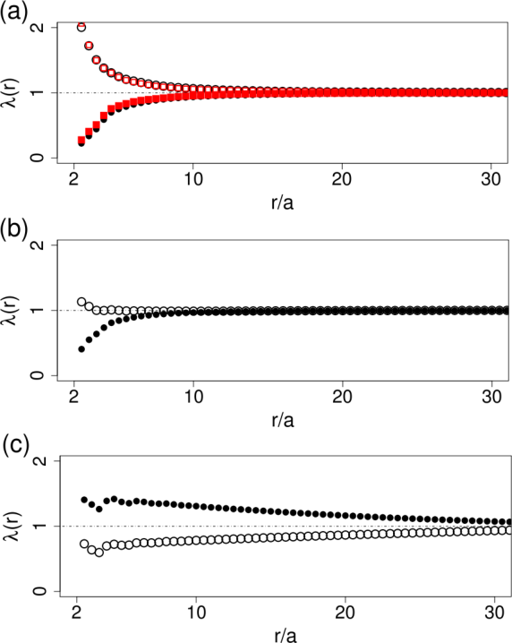
Figure 4a shows the partial densities for same-spin rotors $\lambda_{++}$ and opposite-spin rotors $\lambda_{+-}$ for low rotor density ($\phi_{R}=0.08$) at two passive particle densities $\phi_{P}=0.1,~0.2$. We observe that $\lambda_{+-}\geq\lambda_{++}$ for small $r$, which implies that the opposite spin rotors tend to move together, similar to our previous results without the passive particles [33]. Interestingly, at low rotor density, increasing the passive particle density $\phi_{P}$ from $0.1$ (black marker) to $0.2$ (red marker) does not affect $\lambda_{++}$ or $\lambda_{+-}$.

As the rotor density increases to $\phi_{R}=0.16$, the pairing of opposite spin rotors weakens (figure 4b). However, still $\lambda_{+-}$ is larger than $\lambda_{++}$.

As shown in Figure 4c, increasing the passive particle density $\phi_{P}$, while keeping the rotor density fixed at an intermediate value ($\phi_{R}=0.16$), results in microstructural changes, from the pairs of the opposite spin rotors co-translating ($\lambda_{+-}>\lambda_{++}$) at $\phi_{P}=0.1$ to clusters of the same spin rotors co-rotating ($\lambda_{+-}<\lambda_{++}$) at $\phi_{P}=0.3$. Note that due to the hydrodynamic interactions, rotors of opposite spins tend to co-translate and rotors of same spin co-rotate [35].

These results show that the addition of inert particles to an active rotor bath modifies the rotor-rotor correlations in non-trivial ways. At very low rotor densities, adding more inert particles does not seem to affect the tendency of opposite-spin rotors to co-translate. At slightly higher rotor density however, adding more tracers to the mixture can switch the tendency to rotors from opposite-spin pairings toward same-spin pairings.

Now we try to quantify the clustering and correlations of the rotors and the inert particles by computing the rotor-rotor particle partial densities $\lambda_{RR}$ and rotor-passive particle partial densities $\lambda_{RP}$. Here we do not differentiate the rotors by spin.

Figure 5ab displays the partial densities for the rotor-rotor ($\lambda_{RR}$) and the rotor-passive particles ($\lambda_{RP}$) for the same tracer density ($\phi_{P}=0.1$) but different rotor densities ($\phi_{R}=0.04,~0.24$). At the lower rotor densities, in Figure 5a we observe $\lambda_{RR}>\lambda_{RP}$, indicating that the rotors in general have a higher probability to cluster together. Increasing the rotor density $\lambda_{RR}\approx\lambda_{RP}$, as seen in Figure 5b. However, when the passive particle density is also increased further, clustering or phase separation occurs and $\lambda_{RR}>\lambda_{RP}$ again, as seen in Figure 5c.

It should be noted that, although $\lambda_{RR}>\lambda_{RP}$ is observed both at the lower (Figure 5a) and higher rotor densities $\phi_{R}$ (Figure 5c), the micro-structural origins in these cases are different. As explained in the previous sections (Figures 2, 4), the larger $\lambda_{RR}$ at low rotor density ($\phi_{R}=0.04$) is due to the formation of the doublets of opposite spin rotors co-translating, whereas at high rotor density ($\phi_{R}=0.24$) the co-rotation and clustering of same spin rotors, or phase separation, is responsible for the larger $\lambda_{RR}$.

Here, we investigate the rotor and inert particles’ transport and diffusion by analyzing the mean square displacements.

Figure 6a–c shows the mean-square displacements of the rotors ($\text{MSD}_{R}$) and the passive particles ($\text{MSD}_{P}$). At low rotor density (Figure 6a), $\text{MSD}_{R}>\text{MSD}_{P}$, and rotors transport further than passive particles, but, as the rotor density increases, $\text{MSD}_{R}$ becomes similar to $\text{MSD}_{P}$ (Figure 6b).

Figure 6c shows MSDs at the states where the rotors are self-organized into two counter-rotating vortices. In this phase-separated regime the passive particles move much longer distance than the rotors, mainly because the rotors exhibit spiral motion while trapped in the vortical structures, evident even in the oscillatory patten of $\text{MSD}_{R}$.

In Figure 6d we present the ratio of $\text{MSD}_{P}$ to $\text{MSD}_{R}$. It is clearly shown that at the low rotor densities ($\square$,${\color[rgb]{1,0,0}\circ}$,${\color[rgb]{0,0,1}\triangle}$) $\text{MSD}_{P}\ll\text{MSD}_{R}$. At these low densities, the rotors have a high probability to form a doublet of opposite spin rotors which exhibits translational motion. Considering the collective translational motion of the rotors at low rotor density, it is not surprising to see that $\text{MSD}_{R}>\text{MSD}_{P}$ indicating rotors transport much farther than passive particles.

At increased rotor density the microstructure of the rotor mixture changes from pairs of the opposite spin rotors at low tracer density (${\color[rgb]{0.82,0.62,0.91}+}$) to clusters of the same spin rotors at higher tracer density (${\color[rgb]{255,127,0}\times}$), as explained in the previous subsection. Following the changes in the microstructures of the rotors, the ratio $\text{MSD}_{P}/\text{MSD}_{R}$, which is less than one for low tracer density, becomes larger than one when the tracer density is increased, indicating increased transport of the passive particles.

At high rotor density and low tracer density (${\color[rgb]{0,1,0}\Diamond}$), there is a complete phase separation of the rotors and $\text{MSD}_{P}\gg\text{MSD}_{R}$. When the clusters of same spin rotors emerge, the rotors exhibit closed spiral motion in a cluster, generating a jet-like flow in the interstitial regions. The passive particles translate very long distances as they are carried by these jet-like flows in the boundaries of the clusters, whereas the rotors are trapped in the macroscopic vortices.

In active suspensions, the suspended particles, both rotors and passive particles, exhibit translational as well as rotational motions in response to the flow generated by the active rotors. In other words, the system is driven by the rotational kinetic energy, which is subsequently converted to the translational kinetic energy through the hydrodynamic interactions. We quantify the effects on the systems by tracing the translational and rotational kinetic energies, defined respectively as

where $m$ is the mass of a particle, $I$ is the moment of inertia, and $\langle\cdot\rangle_{A}$ is an ensemble average over the active or passive particles. We also define the ratio

Figure 7a shows changes of the rotors’ translational kinetic energy $T_{R}$ as a function of the passive particle density $\phi_{P}$ for four different rotor densities. At low rotor densities ($\phi_{R}\leq 0.16$), $T_{R}$ does not change significantly with increasing passive particle density. For example, $T_{R}$ for $\phi_{R}=0.16$ is reduced only about 12% when $\phi_{P}$ changes from $0.02$ to $0.3$. Intuitively, for a fixed rotor density, the translational kinetic energy is expected to be a decreasing function of tracer density since the viscous dissipation increases with increasing tracer density. However, at high rotor density $T_{R}$ becomes a non-monotonic increasing function of tracer density.

Figure 7b shows the translational kinetic energy of the passive particles $T_{P}$ as a function of the density of passive particles $\phi_{P}$ for four different rotor densities. For a fixed tracer density, $T_{P}$ is a more sensitive function of rotor density than $T_{R}$. For example, at $\phi_{P}=0.05$, increasing rotor density $\phi_{R}=0.04\rightarrow 0.24$ increases $T_{P}$ 46-fold but increases $T_{R}$ only 9-fold. $T_{P}$ shows a behavior similar to $T_{R}$ at low rotor densities: a decrease of $T_{P}$ at higher passive particle density $\phi_{P}$.

The ratio of the tracer and rotor translational kinetic energies $T_{P}/T_{R}$ is presented in Figure 7c. For the two large rotor densities and small tracer densities, $T_{P}/T_{R}>1$, indicating that the passive particles move faster than the active rotors. However, $T_{P}/T_{R}$ decreases with tracer density and becomes less than one for $\phi_{P}>0.20$. On the other hand, for the two low rotor densities $T_{P}/T_{R}$ is almost uniform. Particularly, for very low rotor density $\phi_{R}=0.08$ this ratio kinetic energies does not change significantly for a wide range of tracer density.

In Figure 7d we plot the ratio $\kappa$ of the translational to the total (translational + rotational) kinetic energy of the rotors. Similar to previous studies [29, 33], $\kappa$ is an increasing function of the rotor density when the passive particle density is held constant. At very low rotor densities $\kappa$ is relatively uniform for the range of $\phi_{P}$ in the present study, whereas for increased rotor density $\kappa$ increases fast with larger $\phi_{P}$.

Figure 7d also shows $\kappa$ of the entire system (passive + active particles)

Notice that $\kappa^{total}$ becomes larger than $\kappa$ of the rotors. It is found that the rotational kinetic energy of the passive particles ($R_{P}$) is negligible compared to $T_{P}$. In other words, $\kappa_{P}\simeq 1$. As a result, adding passive particles to the active rotor system makes the ratio of the translational kinetic energy to the total kinetic energy larger than that of the active rotor system.

References

- [1] M. C. Marchetti, J. Joanny, S. Ramaswamy, T. Liverpool, J. Prost, M. Rao and R. Simha, Rev. Mod. Phys. 85, 1143 (2013).
- [2] J. Dunkel, S. Heidenreich, K. Drescher, H. Wensink, M. Bar and R. Goldstein, Phys. Rev. Lett. 110, 228102 (2013).
- [3] I. Theurkauff, C. Cottin-Bizonne, J. Palacci, C. Ybert and L. Bocquet, Phys. Rev. Lett. 108, 268303 (2012).
- [4] A. Sokolov, I. S. Aranson, J. O. Kessler and R. E.Goldstein, Phys. Rev. Lett. 98, 158102 (2007).
- [5] M. J. Kim and K. S. Breuer, Phys. Fluids, 16, L78 (2004).
- [6] G. Mino, T. E. Mallouk, T. Darnige, M. Hoyos, J. Dauchet, J. Dunstan, R. Soto, Y. Wang, A. Rousselet, and E. Clement, Phys. Rev. Lett., 106, 048102 (2011).
- [7] L. Angelani, C. Maggi, M. L. Bernardini, A. Rizzo, and R. D. Leonardo, Phys. Rev. Lett., 107, 138302 (2011).
- [8] A. Jepson, V. A. Martinez, J. Schwarz-Linek, A. Morozov and W. C. K. Poon, Phys. Rev. E, 88, 041002 (2013).
- [9] T. V. Kasyap, D. L. Koch and M. Wu, Phys. Fluids, 26, 081901 (2014).
- [10] A. E. Patteson, A. Gopinath, P. Purohit and P. E. Arratia,arXiv, 1505.05803v2 (2015).
- [11] Y. Peng and et al., Phys. Rev. Lett., -, in press (2016).
- [12] X.-L. Wu and A. Libchaber, Phys. Rev. Lett., 84, 13 (2000).
- [13] K. C. Leptos, J. S. Guasto, J. P. Gollub, A. I. Pesci and R. E. Goldstein, Phys. Rev. Lett., 103, 198103 (2009).
- [14] R. Jeaneret, V. Kantsler and M. Polin, arXiv, 1602.01666 (2016).
- [15] Z. Lin, J. Thiffeault and S. Childress, J. Fluid Mech., 669, 167- 177 (2011).
- [16] D. Pushkin, H. Shum and J. M.Yeomans, J. Fluid Mech., 726, 5-25 (2013).
- [17] D. F. Hinz, A. Panchenko, T.-Y. Kim and E. Fried, Soft Matter, 10, 9082 (2014).
- [18] S. Li, H. Jiang and Z. Hou, Soft Matter, 11, 5712 (2015).
- [19] S.Takatori and J.F. Brady, Soft Matter, 11,7920-7931 (2015).
- [20] Y. Fily and M. Marchetti, Phys. Rev. Lett, 108, 235702 (2012).
- [21] G. Redner, M. Hagan and A. Baskaran, Phys. Rev. Lett., 110, 055701 (2013).
- [22] J . Stenhammar, R. Wittkowski, D. Marenduzzo and M. E. Cates, Phys. Rev. Lett., 114, 018301 (2015).
- [23] A. Snezhko, Current Opinion in Colloid & Interface Science, in press (2016).
- [24] G. Kokot, A. Snezhko and I. S. Aranson, Soft Matter, 9, 6757 (2013).
- [25] G. Kokot, D. Piet, G. M. Whitesides, I. S. Aranson and A. Snezhko, Sci. Rep., 5 (2015).
- [26] A. Snezhko and I. S. Aranson, Soft Matter,11, 6055 (2015).
- [27] A. Bricard, J. Caussin, N. Desreumaux, O. Dauchot, and D. Bartolo, Nature, 503, 95-98 (2013).
- [28] A. Bricard, J.-B.Caussin, D. Das, C. Savoie, V. Chikkadi, K. Shitara, O. Chepizhko, F. Peruani, D. Saintillan, and D.Bartolo , Nat. Comm., 6, 7470 (2015).
- [29] N. H. P. Nguyen, D. Klotsa, M. Engel, and S. C. Glotzer, Phys. Rev. Lett. 112, 075701 (2014).
- [30] M. Spellings, M. Engel, D. Klotsa, S. Sabrina, A. M. Drews, N. H. P. Nguyen, K. J. M. Bishop and S. Glotzer, Proc. Natl. Acad. Sci. USA, 112, E4642?E4650 (2015).
- [31] S. Sabrina, M. Spellings, S. C. Glotzer and K. J. M. Bishop, Soft Matter, 11, 8409-8416 (2015).
- [32] Y. Goto and H. Tanaka, Nat. Comm. 6 (2015).
- [33] K. Yeo, E. Lushi, and P. M. Vlahovska Phys. Rev. Lett. 114, 188301 (2015).
- [34] E. Lushi, H. Wioland and R. E. Goldstein, Proc. Natl. Acad. Sci. USA, 111, 9733-9738 (2014).
- [35] E. Lushi and P. M. Vlahovska, J. Nonlin. Sci., 25, 1111- 1123 (2015).
- [36] M. Leoni and T. Liverpool, Europhysics Letters, 92 (2010).
- [37] Y. Fily, A. Baskaran and M. C. Marchetti, Soft Matter, 8, 3002-3009 (2012).
- [38] S. Kim and S. J. Karrila, Microhydrodynamics: Principles and Selected Applications, Butterworth-Heinemann, 1991.
- [39] J. Stickel and R. L. Powell, Ann. Rev. Fluid Mech., 37, 129 (2005).
- [40] K. Yeo and M. Maxey, J. Comp. Phys., 229, 2401-2421 (2010).
- [41] E. Climent, M. R. Maxey and G. E. Karniadakis, Langmuir, 20, 507-513 (2004).
- [42] K. Yeo and M. R. Maxey, Phys. Rev. E, 81, 062501 (2010).
- [43] B. Grzybowski, H. A. Stone and G. M. Whitesides, Nature 405, 1033-1036 (2000).
- [44] B. Grzybowski and G. M. Whitesides, Science, 296, 718- 721(2002).
- [45] M. Friese, T. Nieminen, N. Heckenberg and H. Rubinsztein- Dunlop, Nature, 394, 348-350 (1998).
- [46] A. Petroff, X.-L. Wu and A. Libchaber, Phys. Rev. Lett., 114, 158102 (2015).
- [47] K. Drescher, K. Leptos, I. Tuval, T. Ishikawa, T. Pedley and R. E. Goldstein, Phys. Rev. Lett., 102, 168101 (2009).
- [48] J. Schwarz-Linek, C. Valeriani, A. Cacciuto, M. E. Cates, D. Marenduzzo, A. N. Morozov and W. C. K. Poon, Proc. Natl. Acad. Sci. USA, 109, 4052-4057 (2012).