Note on “Diffusive quantum criticality in three-dimensional disordered Dirac semimetals”

We here clarify some errors in our previous two-loop calculation for potential disorder driven Dirac semimetal (DSM)-compressible diffusive metal (CDM) quantum phase transition (QPT) in three spatial dimensions ($d=3$), presented in Ref. [1]. In Ref. [1], we performed a two-loop analysis within the framework of an $\epsilon$-expansion near $d=2$ (the lower critical dimension for the problem), and reported that the correlation length exponent (CLE) ($\nu$) is given by $\nu^{-1}=\epsilon-\frac{\epsilon^{2}}{8}+{\mathcal{O}}(\epsilon^{3})$ and dynamic scaling exponent (DSE) $z=1+\frac{\epsilon}{2}-\frac{3}{16}\epsilon^{2}+{\mathcal{O}}(\epsilon^{3})$, where $\epsilon=d-2$, near the DSM-CDM quantum critical point (QCP). Hence, for $d=3$, we found $\nu\approx 1.14$ and $z\approx 1.31$ [1]. We now realized that the quoted values of these two exponents are incorrect, because we missed some relevant two-loop diagrams, which we correct here. But, more importantly we here question the validity of such an $\epsilon$-expansion near $d=2$ and argue that the $\epsilon$-expansion may not be reliable for this problem.

We realized that instead of reevaluating the diagrams shown in Ref. [1], one can derive the flow equation for disorder coupling ($\Delta$) by analyzing the Gross-Neveu (GN) model for a discrete chiral symmetry breaking mass condensation for which the flow equation of GN coupling ($g$) is known to three-loop order [2, 3, 4, 5]. The Euclidean actions for these two theories are respectively

where $\bar{\Psi}=\Psi^{\dagger}\gamma_{0}$, $a,b$ are replica indices. Due to fermion doubling in a lattice, we work with four dimensional $\gamma$ matrices, satisfying the anticommutaiton relation $\left\{\gamma_{\mu},\gamma_{\nu}\right\}=2\delta_{\mu\nu}$. Critical behavior of $S_{GN}$ and $\bar{S}_{D}$ can be studied performing $\epsilon$-expansions respectively near two space-time and spatial dimensions. The infra-red flow equation for $g$ to three-loop order reads as [2, 3, 4, 5]

where $\epsilon=D-2$ with $D$ as space-time dimensions, and $n$ is the number of spinor components.

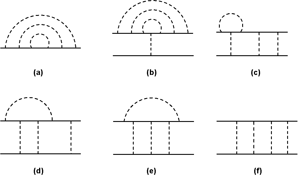
To derive the flow equation of $(\Delta)$ one can set the external frequency to zero, for which we establish a correspondence between diagramatic contributions for $S_{GN}$ and $\bar{S}_{D}$. Contributions from relevant (i) one-loop (Fig. $(i)$-$(iv)$ of Ref. [1]) and three-loop [see Fig. 1] diagrams are of opposite sign when the fermion vertex is accompanied by the matrix $\mathbb{1}_{4\times 4}$ (GN theory) and $\gamma_{0}$ (potential disorder), (ii) two-loop diagrams that renormalize either GN ($g$) or disorder ($\Delta$) coupling are of same sign for these two theories. Thus we can arrive at the flow equation for $(\Delta)$ to three-loop order from Eq. (3) by (i) first setting $n=0$, since any contribution proportional to $n$ involves fermion bubble that vanishes in the vanishing replica limit, and (ii) taking $-g=\Delta$, leading to

where $\epsilon=d-2$ and $d$ represents the spatial dimensions. The exact location of the DSM-CDM QCP to from one-, two and three-loop order are respectively $\Delta^{\ast}_{(1)}=\epsilon/2$, $\Delta^{\ast}_{(2)}=\left(-1+\sqrt{1+2\epsilon}\right)/2$ and

When we expand the last two quantities in powers of $\epsilon$ the radius of convergence is $1/2$ and $\leq 0.35$ (extracted numerically). Thus, setting $\epsilon=1$ to extract the CLE in $d=3$ is not a well defined procedure, since this expansion is not asymptotically convergent. Therefore, higher order terms from the $\epsilon$-expansion about two spatial dimensions only produces unreliable results for $\epsilon=1$ and this methodology of addressing the critical properties of DSM-CDM QPT in $d=3$ needs to be abandoned.

Even if we choose to extract CLE from the powers series in terms of $\epsilon$, to one-, two- and three-loop orders we respectively find $\nu^{-1}_{(1)}=\epsilon+{\mathcal{O}}(\epsilon^{2})$,

Therefore, in three spatial dimensions ($\epsilon=1$), we obtain $\nu_{(1)}=1$, $\nu_{(2)}\approx 0.67$ and $\nu_{(3)}\approx 0.53$. The fact that the inclusion of higher order corrections pushes the CLE close to the mean-field value ($\nu=1/2$) is alarming, indicating failure of $\epsilon$-expansion to capture the critical properties. It may be worthwhile to mention that the higher loop results for the CLE either do not ($\nu_{(3)}$) or barely ($\nu_{(2)}$) satisfy the Chayes-Chayes-Fisher-Spencer inequality $(\nu>2/d)$ [6], while the one-loop result $(\nu=1)$ satisfies the inequality, indicating that going beyond the one-loop order may not be meaningful in this problem.

Furthermore, one may wish to capture the asymptotic behavior of CLE using the Padé approximation [7, 8]. For $\nu^{-1}_{(2)}$ a Padé $[1|1]$ approximation yields

Consequently, we obtain a mean-field value of CLE $\nu_{(2)}=1/2$ for $\epsilon=1$. On the other hand, to estimate the asymptotic behavior of $\nu^{-1}_{(3)}$ we can employ either Padé $[2|1]$ or Padé $[1|2]$ approximations, respectively yielding

in turn giving $\nu_{(3)}\approx 0.33$ and $0.375$ for $\epsilon=1$, both being smaller than the mean-field value of CLE, strongly suggesting the inapplicability of $\epsilon$-expansion for $d=3$.

We do not discuss the corrections to the DSE ($z$) beyond the leading order in $\epsilon$. Given that the radius of convergence of $\Delta^{\ast}_{(2,3)}\ll 1$, we conclude that higher order corrections to $z$ are not meaningful when $\epsilon=1$.

Therefore, within the $\epsilon$-expansion scheme, where $\epsilon=d-2$, only reliable values of the critical exponents near DSM-CDM QCP are $\nu=\epsilon^{-1}$ and $z=1+\epsilon/2$, respectively giving $\nu=1$ and $z=3/2$ in three spatial dimensions ($\epsilon=1$), which one can also obtain from one-loop Wilsonian renormalization group analysis [9]. Going to higher loop calculations in $\epsilon$ for $d=3$ can only produce progressively worse results for the critical exponents since the corresponding series is manifestly not convergent.

We point out that recent numerical calculations for the DSE ($z$) agree with the result from one-loop $\epsilon$-expansion within numerical error bars [10, 11, 12, 13, 14], whereas the one-loop result for CLE ($\nu$) reasonably agrees (within error bar) with the numerically calculated exponents in Ref. [10, 12, 13, 14], but disagrees with Ref. [11]. Whether the agreement between the numerical results and the one-loop calculation is merely a coincidence or implies something deep about the problem is unknown at this stage.

B. R. is thankful to John Gracey for valuable communication related to perturbative analysis of Gross-Neveu model. B. R. also thanks Igor Herbut and Pallab Goswami for useful discussion on this problem. During the preparation of the erratum, we became aware of a preprint [15] where a two-loop calculation has been carried out explicitly. Our flow equation in Eq. (4) to two-loop order agrees with the one reported in Ref. [15].

References

- [1] B. Roy, and S. Das Sarma, Phys. Rev. B 90, 241112(R) (2014).
- [2] J. A. Gracey, Nucl. Phys. B 367, 657 (1991).
- [3] C. Luperini, and P. Rossi, Annals of Physics 212, 371 (1991).
- [4] N. A. Kivel, A. A. Stepanenko, and A. N. Vasil’ev, Nucl. Phys. B 424, 619 (1994).
- [5] M. Moshe, and J. Zinn-Justin, Physics Reports 385, 69 (2003).
- [6] J. T. Chayes, L. Chayes, D.?S. Fisher, and T. Spencer, Phys. Rev. Lett. 57, 2999 (1986).
- [7] G. A. Baker, P. Graves-Morris, Padé Approximants, (Cambridge University Press, 2nd ed., 1996).
- [8] Since the power series of CLE does not display oscillatory behavior we cannot perform a Borel summation.
- [9] P. Goswami, and S. Chakravarty, Phys. Rev. Lett. 107, 196803 (2011).
- [10] K. Kobayashi, T. Ohtsuki, K.-I. Imura, and I. F. Herbut, Phys. Rev. Lett. 112, 026602 (2014).
- [11] B. Sbierski, E. J. Bergholtz, P. W. Brouwer, Phys. Rev. B 92, 115145 (2015).
- [12] J. Pixley, P. Goswami, and S. Das Sarma, Phys. Rev. B 93, 085103 (2016).
- [13] S. Liu, T. Ohtsuki, R. Shindou, arxiv:1507.02381
- [14] S. Bera, J. D. Sau, B. Roy, arxiv:1507.07551
- [15] S. V. Syzranov, P. M. Ostrovsky, V. Gurarie, L. Radzihovsky, arXiv:1512.04130