Measuring Blood Glucose Concentrations in Photometric Glucometers Requiring Very Small Sample Volumes

Our underlying assumption is that the glucose images will contain a ROI, where the blood sample is distributed and, thus, the color change of the ROI represents the reflectivity caused by the underlying glucose concentration. This area will not necessarily be completely spatially connected as it may contain artefacts where the reaction has not taken place, or granularities in the chemical that do not contribute to a proper reaction. Other areas in the image will not correspond to the ROI, either, because the blood sample is unevenly distributed in these areas, or because the areas are dry, i.e., not covered with blood. We interpret the different areas contained in the image as clusters with specific cluster centres overlaid by noise. We assume that data points converging to a certain cluster center will belong to the corresponding area. The noise here is assumed to be Gaussian. This assumption is based on the calibration frames where no reaction has started.
The mean-shift algorithm [18] has become a popular approach for clustering and mode location estimation. It has been widely applied for medical image segmentation as it does not require the knowledge of the actual number of clusters [8, 19, 20, 21, 22]. We use the mean-shift algorithm (MS), as well as two extensions of it: the robust mean-shift (R-MS) [9] and the scalable, sparse mean-shift (SS-MS) [10]. Furthermore, we extend these variants to the medoid-shift [23].
Assume a set of $L$ pixels in a gray-scale image¹¹ 1 Including spatial information for gray-scale images will increase the dimensions by two, leading to a three-dimensional data vector ${{\mathbf{x}}=[x^{\text{intensity}},x^{\text{position},M_{x}},x^{\text{position},M_{y}}]}$. at frame $n$ that can be expressed as $x_{l}^{(n)}\in\mathbb{R}$, $l=1,\ldots,L$ as in Eq. (1). We will omit the frame notation, henceforth, for better readability.
A consistent estimator of the density is given by the kernel density estimator (KDE) [24] with bandwidth parameter $h$

where $K({\mathbf{x}})$ is a radially symmetric kernel function with a strictly decreasing profile for $x\geq 0$. The bandwidth ${h}$ of the kernel function is the only parameter that has to be tuned and is crucial to the performance of the mean-shift algorithm, as it affects the number of clusters. Extensive work has dealt with the choice of the bandwidth parameter, e.g. [25, 24].
Generally, the mean-shift algorithm is derived by taking the zeros of the gradient of the KDE

and reformulating to get the mean-shift vector of ${\mathbf{x}}$ as

where $K^{\prime}=\frac{dK}{d{\mathbf{x}}}$. Each data point is shifted according to Eq. (7) in the direction of steepest ascent until convergence, such that the sequence of successive locations of a data vector

where ${\mathbf{x}}^{(j)}$ denotes the $j$-th iteration step. Typically, the mean-shift algorithm tends to overestimate the number of modes. It is usual to post-process the mean-shift results with a simple clustering method to group nearby modes together, e.g. using a mode pruning step with bandwidth $h$ [8, 19].
Another way to express the KDE, which allows for extensions of the mean-shift, is to consider the kernel to be an inner product in the Hilbert space $\mathcal{H}$, such that[26]

where $\Phi:\mathbb{R^{d}}\rightarrow\mathcal{H}$ is a mapping function and $\langle\cdot\rangle$ denotes the inner product. $K(\frac{{\mathbf{x}}-x_{l}}{h})$ is a positive definite kernel function. Hence, the KDE can be formulated as

In this formulation, the uniform weights $\frac{1}{L}$ have been substituted by $w_{l}>0$ to attain a more general form. It has been shown [19] that the mean-shift algorithm converges and that the mode estimator is asymptotically consistent and unbiased.

In [9], the robust mean-shift (R-MS) is derived as an alternative to account for heavy-tailed noise in the data. Here, the sample mean of vectors in Eq. (10) is substituted by a robust M-estimate

where $\rho\!\left(\cdot\right)\,$ is a monotone, differentiable loss function, such as Huber’s loss function [27] and the scale $\hat{\sigma}$ is initialized with a robust estimate based on the mean absolute deviation [9]. This leads to the robust KDE

where the robust weights $w_{l}^{\text{R-MS}}$ can be determined using Iteratively ReWeighted Least Squares (IRWLS) [9, 28], resulting in

where $\psi=\rho^{\prime}$. The robust mean-shift vector reads

For a more detailed description of the R-MS the reader is referred to [9].

The computational complexity of the mean-shift algorithm is proportional to the square of the total number of data points $L$. To overcome the problem of high computational demand, a scalable sparse version has been derived in [10]. A more detailed discussion of the computational complexity of both versions is provided in [10]. Using only a subset of the data points, the SS-MS is able to achieve high accuracy while reducing computational power. The gist lies in substituting the mean in Eq. (10) by a sparse approximation[29, 30]. A short outline will be given in the sequel, for more details the reader is referred to [10]. The sparse approximation of the mean can be formulated as

where the index set $\mathcal{I}\subseteq\{1,\ldots,L\}$ of cardinality $|\mathcal{I}|=N$ is defined to be a subset of the full set of indices, the weights follow $\bm{\alpha}\in\mathbb{R}^{N}$ and $1\leq N\ll L$. The scalable, sparse KDE

where $\alpha_{\mathcal{I}^{*},i}$ denotes the $i$-th weight obtained using the optimal set $\mathcal{I}^{*}$. The resulting mean-shift vector has the form

A robust sparse formulation (RSS-MS) can be derived [10].
To solve Eq. (16), we need to: 1) find a solution for the inner optimisation problem; i.e., solve for $\bm{\alpha}$: 2) find an optimal set $\mathcal{I}^{*}$. For a fixed $\mathcal{I}$, $\bm{\alpha}_{\mathcal{I}}=\bm{\Xi}^{-1}_{\mathcal{I}}\bm{\xi}_{\mathcal{I}}$. Here

where $\bm{\Xi}_{\mathcal{I}}$ is the Gram matrix. To ensure convergence, ${\alpha_{i}<0,\forall i=1,...,N}$. Generally, $\alpha_{i}$ will not always fulfill the property. We, therefore, normalise the weights $\alpha_{i}$ by setting to zero all weights $\alpha_{i}<0$ and re-normalising such that $\sum_{i}\alpha_{i}=1$. The optimal index subset is found by assuming a fixed $N$ and maximising an incoherence function $\nu_{\mathcal{I}}$

where

This is intuitive in the sense that to find the most representative subset of data vectors, we choose the ones that are most incoherent to each other. In [10], we outline an algorithm to maximize $\nu_{\mathcal{I}}$ and determine $\mathcal{I}^{*}$. The question remaining is how to choose the cardinality $N$ of the subset of indices $\mathcal{I}$. Clearly, in some cases this can be given by the application at hand knowing a certain $N_{\text{max}}$, or by using test data for cross-validation, as in [10], where $N$ is set to be sufficiently high to incorporate the worst-case scenario. We introduce a data-driven selection of $N$, which results in a smaller $N$ for most data sets than cross-validation. Figure 6 shows typical examples of the progression of a normalised version of $\nu_{\mathcal{I}}$

for the images given in Fig. 3, using different values of $N=1,\ldots,L$. We observe that the value of $\widetilde{\nu}_{\mathcal{I}}$ drops quickly after a certain value of $N$ and that the behaviour of the curve is similar for different images. This signifies that the first $N_{\nu}$ samples chosen by the algorithm contribute highly to the incoherence in the image and it is sufficient to use a subset $\mathcal{I}$ of cardinality $N_{\nu}$ for the sparse representation.

We propose to choose $N_{\nu}$ based on the gradient of $\widetilde{\nu}_{\mathcal{I}}$ in Fig. 6 and set a threshold $T_{\nu}$

The choice of $T_{\nu}$ is based on heuristics and chosen specifically for the data at hand by observing the trade-off between accuracy and computation.

It remains to prove that the mean-shift algorithm in all its variations will converge. In [19], the convergence proof of the standard MS is given. We extend it for the cases of the R-MS and the SS-MS.

The proof given in Appendix A is a generalised version of Theorem 1 in [19]. We need to ensure that the weights will fulfill $w_{l}^{\text{R-MS}}>0$ for R-MS and $\alpha_{{\mathcal{I}}^{*},i}>0$ for SS-MS. $w_{l}^{\text{R-MS}}$ are derived using the IRWLS and are, thus, certain to follow the required property for monotone loss functions $\rho\!\left({\cdot}\right)\,$. The calculation of $\alpha_{{\mathcal{I}}^{*},i}$ ensured that it follows this property.

The coefficient of variation (CV) is a very popular measure to assess the accuracy of pharmacokinetic measurements [31]. In our work, we use the remission coefficient of variation $\text{CV}_{\hat{r}}$

where $\gamma=1,\ldots,N_{g}$, $\hat{\sigma}_{\mathcal{\hat{R}}_{g(\gamma)}}$ and $\hat{\mu}_{\mathcal{R}_{g(\gamma)}}$ are the sample standard deviation, and respectively the sample mean of the elements of the set $\mathcal{\hat{R}}_{g(\gamma)}$. $\mathcal{\hat{R}}_{g(\gamma)}$ denotes the test set of relative remission estimates obtained from several measurements of the same underlying glucose concentration $g(\gamma)$.

The Clarke Error Grid (CEG) [32] is a standard method for evaluating glucose measurement performance. It plots the estimated glucose concentrations against the actual glucose concentrations and classifies the error according to its medical severity. To this end, different regions are defined in the CEG as depicted in Fig. 13. A common specification is to have at least $95\%$ of all points in the region A, maximally $5\%$ of all points in the region B [33] and no points in the other zones.

To quantify the validation, we employ a glucose specific mean absolute deviation (MAD) inspired by [32]. Instead of using the standard MAD between the true and the estimated glucose level, a glucose-specific MAD (gMAD) is defined. The gMAD weighs the errors using a penalty function according to their medical severity on the basis of the CEG. Hereby, errors made for hypoglycaemic cases below $70\text{\,}\mathrm{m}\mathrm{g}\mathrm{/}\mathrm{d}\mathrm{l}$ are weighed with the highest factor $w_{\text{gMAD}}$ as they present critical short-term risks; hyperglycaemic cases which present more long-term risks are weighed with a slightly smaller factor $w_{\text{gMAD}}$, and normal cases are given the factor $w_{\text{gMAD}}=1$. The gMAD reads

where the penalty function is given by

with $\overline{\sigma}(\cdot)$ and ${\sigma}(\cdot)$ being sigmoid functions that ensure a smooth transition as given in [32]. According to the most recent ISO standards [34], the maximal permissible error is $\pm$15\text{\,}\mathrm{m}\mathrm{g}\mathrm{/}\mathrm{d}\mathrm{l}$$ within a reference range of $0\text{\,}\mathrm{m}\mathrm{g}\mathrm{/}\mathrm{d}\mathrm{l}75\text{\,}\mathrm{m}\mathrm{g}\mathrm{/}\mathrm{d}\mathrm{l}$ and $20\%$ for a reference range above $75\text{\,}\mathrm{m}\mathrm{g}\mathrm{/}\mathrm{d}\mathrm{l}$.

In Fig. 8, we present a selection of the results of the kinetic curves, i.e., the progression of the relative remission over time for the different data sets, using MS (mean-shift), RSS-MS (robust sparse MS), MedS (medoid-shift), and R-MedS (robust MedS).

For the time being, we will present the results using the standard convergence criterion, i.e., when the slope reaches a threshold of $T_{\text{slope}}$ for a series of consecutive frames. Overall, we establish the expected progression of the kinetic curve with its three typical stages as in Fig. 2. We see that measurements of the same underlying glucose concentration are, mostly, bundled together. Convergence is reached faster for low glucose concentrations than for high glucose concentrations. Moreover, our assumption that the decay rate $\tau$ of the reaction is correlated with the underlying glucose concentration is confirmed. The higher the underlying glucose concentration, the steeper the decay.
We observe a significant decrease in performance when comparing Set E with Set F, which were taken using the exact same setup and blood samples, however using different volumes of the blood samples.

These results are underlined when analyzing the resulting $\text{CV}_{\hat{r}}$ values for these two sets in the left part of Table II. This indicates that blood sample volumes in the range of $1\text{\,}\mathrm{n}\mathrm{l}$ could be problematic. The volume range $10\text{\,}\mathrm{n}\mathrm{l}100\text{\,}\mathrm{n}\mathrm{l}$, in contrast, seems to perform well.
Table II shows that the medoid-shift versions are significantly better than the mean-shift versions for all sets. Observing Set B, we notice that the difference in performance between the two methods is not as high as for other sets. The reason can be understood from Fig. 9. The more distinct the modes are, the more separable the clusters, the better mean-shift performs. By choosing the medoid instead of the mean and converging to actual points in the data set, the medoid-shift doesn’t show this bias in estimators.
The results for the sparse scalable mean-shift are given in the right part of Table II. We assert that the resulting $\text{CV}_{\hat{r}}$ values are slightly worse than their non-scalable counterparts. This degradation, however, is not too severe and the loss in accuracy can be accepted to ensure lower computation. Only for Set E do we notice a severe degradation in performance, when using the SS-MS. This can be traced back to the fact that due to the very small blood volume, the ROI is much smaller than for the other measurements.

As portrayed in Section III-C3, we propose a data-driven approach to select $N_{\nu}$ uniquely for every frame. Figure. 10 shows the choice of $N_{\nu}$ for Set C, with $N_{\nu}$ averaged over all frames for each measurement. The tendency matches our expectations: very low glucose concentrations are characterized by low contrast and therefore higher coherence. The choice of $N_{\nu}$ is higher than for high glucose concentrations, i.e., more data points are needed to reliably represent the image. As the concentration increases and the images become more distinct in the different regions, the variance in the choice of $N_{\nu}$ for the same glucose concentrations decreases. Taking the worst-case scenario would have resulted in $N\approx 370$ data points, which is much higher than the data-driven choice of $N$.

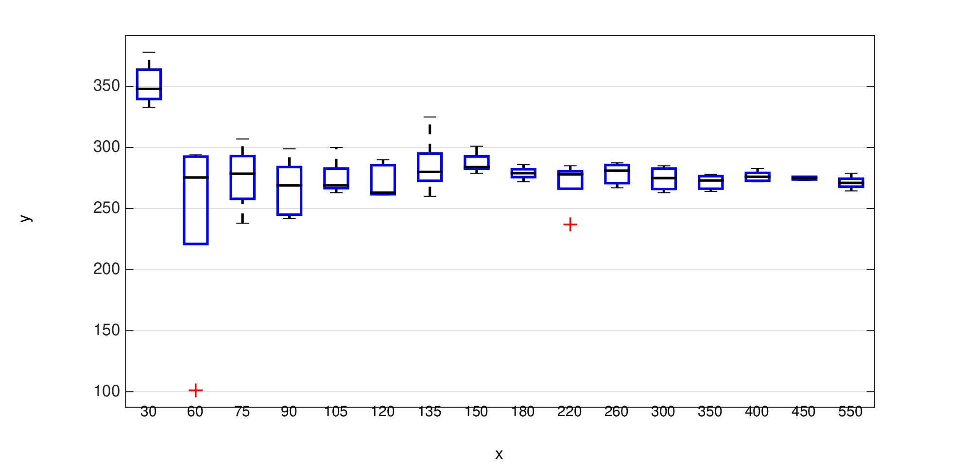
Let us now analyze the quality of the SS-MS when using a data-driven choice of $N_{\nu}$ versus a fixed $N_{\nu}=0.37L$. The results are given for the RSS-MedS in Table. III. Evidently, the accuracy of both approaches is comparable. This underlines that a data-driven $N_{\nu}$ maintains the accuracy needed.

The kinetic curves in Fig. 8 show that convergence for same-glucose-level measurements is not always reached at the same time which results in strongly varying remission estimates, although the course of the kinetic curve is very similar.

Let us take the $550\text{\,}\mathrm{m}\mathrm{g}\mathrm{/}\mathrm{d}\mathrm{l}$ measurements in Fig. 8 (b) as an example. Convergence is found at times between $\hat{t}_{C}\approx$4\text{\,}\mathrm{s}$$ and $\hat{t}_{C}\approx$9\text{\,}\mathrm{s}$$, leading to remission estimates from $\hat{r}_{C}\approx 50\%$ to $\hat{r}_{C}\approx 59\%$. Figure 11 (a) shows the EKF state estimates $\hat{r}_{C}^{(\text{EKF Conv})}$ for this example. Evidently, the EKF converges to reliable state estimates quickly and therefore, the resulting $\hat{r}_{C}$ estimates not only lie in the same range, but match the final convergence value of the kinetic behavior more accurately. This can be seen clearly in Fig. 11 (b). The convergence value reached by the standard method $\hat{r}_{C}^{(\text{Stand. Conv})}$ occurs after around $11\text{\,}\mathrm{s}$ and does not match the actual saturation value. The convergence value reached by EKF $\hat{r}_{C}^{(\text{EKF Conv})}$, however, occurs after $5\text{\,}\mathrm{s}$ and is much closer to the actual saturation value.

Table IV shows the time gain obtained using the EKF. These results are the average of all time gain values obtained for all sets over all measurements. Comparing the remission estimates $\hat{r}_{C}^{(\text{Stand. Conv})}$ and $\hat{r}_{C}^{(\text{EKF Conv})}$ to the saturation values of the chemical reaction, we assert that the EKF produces more accurate results, with a gain of more than $2\%$ in remission.
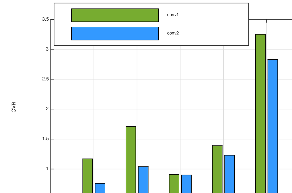
Figure 12 presents a comparison of $\text{CV}_{\hat{r}}$ values and gMAD values for the standard convergence criterion and the EKF convergence method. This analysis considers for each set the method with the best results in Tables II and V, respectively, and compares it to its EKF-method-equivalent. The EKF convergence always leads to improved $\text{CV}_{\hat{r}}$ values. Similarly, for the high glucose range the gMAD results show the same outcome. For low glucose ranges the standard convergence compares favourably. The reason for this is that the EKF method is quite sensitive to the model used. As can be seen in Fig. 8, the kinetic curves of low glucose measurements exhibit a dip after the drop followed by a steady rise. This is not embodied in the model in Eq. (29).

Finally, we present the results of the glucose estimates $\hat{g}$ obtained by mapping the remission estimates using $f_{\text{Calib}}$.

The Clarke Error Grid plot of Set E in Fig. 13 (a) shows that 93 $\%$ of the points lie in region A, 6 $\%$ lie in region B and $1\%$ lie in region D using the standard convergence criterion. Thereby, the results do not conform with the requirements. As indicated by the results in Fig. 13 (b), using EKF state estimation to predict the convergence values leads to a significant improvement of the results. Now 100$\%$ of the estimates of Set E lie in the A-region.

Table V presents the mean gMAD values for $\hat{g}$ of each set separated according to the glucose range. This analysis is omitted for Sets A and D, as they do not contain enough different glucose concentrations to construct the mapping function. The results for most sets lie below the ISO requirements, i.e., low glucose ranges show errors smaller than gMAD $=\pm$15\text{\,}\mathrm{m}\mathrm{g}\mathrm{/}\mathrm{d}\mathrm{l}$$ and high glucose ranges show an error larger than 20$\%$. However, we note that in Set E the limit is often exceeded, confirming again the fact that blood sample volumes around $1\text{\,}\mathrm{n}\mathrm{l}$ are problematic.
The previously made observation concerning medoid-shift outperforming mean-shift is confirmed again here. The robust version seems to improve the performance in high glucose ranges more than in low glucose ranges.

References

- [1] “http://www.who.int/diabetes/en/, retrieved October 2015,” .
- [2] “http://www.diabetes.co.uk, retrieved October 2015.,” .
- [3] The Diabetes Control and Complications Trial Research Group, “The effect of intensive treatment of diabetes on the development and progression of long-term complications in insulin-dependent diabetes mellitus,” New England Journal of Medicine, vol. 329, no. 14, pp. 977–986, 1993.
- [4] B. Guerci et al., “Self-monitoring of blood glucose significantly improves metabolic control in patients with type 2 diabetes mellitus: the auto-surveillance intervention active (asia) study,” Diabetes and Metabolism, vol. 29, no. 6, pp. 587 – 594, 2003.
- [5] J.M. Asfour et al., “Analyse Optischer Daten Mit Hilfe Von Histogrammen.,” Dec. 07 2011, European Patent Application, EP1843148A1.
- [6] M.J. Tierney J.A.Tamada, M.Lesho, “Keeping watch on glucose,” IEEE Spectrum, vol. 39, no. 4, pp. 52–57, 2002.
- [7] Stefan Leier, “Methods of signal detection and processing in medical engineering,” M.S. thesis, TU Darmstadt, 2009.
- [8] N. Demitri and A.M. Zoubir, “Mean-shift Based Algorithm for the Measurement of Blood Glucose in Hand-Held Devices,” in Proceedings of the 21st European Signal Processing Conference (EUSIPCO), September 2013.
- [9] N. Demitri and A.M. Zoubir, “A Robust Kernel Density Estimator Based Mean-Shift Algorithm,” in IEEE 39th International Conference on Acoustics, Speech, and Signal Processing (ICASSP), May 2014.
- [10] N. Demitri and A.M. Zoubir, “Estimating glucose concentration using a sparse scalable mean-shift algorithm.,” in 2015 IEEE 11th International Symposium on Biomedical Imaging (ISBI), April 2015.
- [11] S.F. Clarke and J. R. Foster, “A history of blood glucose meters and their role in self-monitoring of diabetes mellitus,” British Journal of Biomedical Science, vol. 69 (2), pp. 83–93, March 2012.
- [12] K.-J. Lee J.-Y. Shin, H.-H. Nam, “Estimation of glucose concentration using adaptive calibration curve in different hematocrit levels,” Electronics Letters, vol. 49, no. 9, pp. 584–585, 2013.
- [13] S. Kayashima et al., “New noninvasive transcutaneous approach to blood glucose monitoring: successful glucose monitoring on human 75 g OGTT with novel sampling chamber,” IEEE Transactions on Biomedical Engineering, vol. 38, no. 8, pp. 752–757, Aug 1991.
- [14] M. Yamaguchi, M. Mitsumori, and Y. Kano, “Noninvasively measuring blood glucose using saliva,” IEEE Engineering in Medicine and Biology Magazine, vol. 17, no. 3, pp. 59–63, May 1998.
- [15] B.D. Cameron and G.L. Cote, “Noninvasive glucose sensing utilizing a digital closed-loop polarimetric approach,” IEEE Transactions on Biomedical Engineering, vol. 44, no. 12, pp. 1221–1227, Dec 1997.
- [16] E. Baumann, W. Obermeier, and K. Werner, “Light source pulsed with irregular pulse sequence in analog photometric signal evaluation for a test carrier analysis system,” Oct. 31 1995, US Patent 5,463,467.
- [17] Steven M. Kay, Fundamentals of Statistical Signal Processing: Estimation Theory, Prentice-Hall, Inc., Upper Saddle River, NJ, USA, 1993.
- [18] K. Fukunaga and L. Hostetler, “The estimation of the gradient of a density function, with applications in pattern recognition,” IEEE Transactions on Information Theory, vol. 21, no. 1, pp. 32–40, 1975.
- [19] D. Comaniciu and P. Meer, “Mean shift: a robust approach toward feature space analysis,” IEEE Transactions on Pattern Analysis and Machine Intelligence, vol. 24, no. 5, pp. 603–619, 2002.
- [20] M. A. King et al., “Counting moles automatically from back images,” IEEE Transactions on Biomedical Engineering, vol. 52, no. 11, pp. 1966–1969, 2005.
- [21] A. Janowczyk et al., “High-throughput biomarker segmentation on ovarian cancer tissue microarrays via hierarchical normalized cuts,” IEEE Transactions on Biomedical Engineering, vol. 59, no. 5, pp. 1240–1252, May 2012.
- [22] O. Debeir et al., “Tracking of migrating cells under phase-contrast video microscopy with combined mean-shift processes,” IEEE Transactions on Medical Imaging, vol. 24, no. 6, pp. 697–711, June 2005.
- [23] Y. A. Sheikh, E. A. Khan, and T. Kanade, “Mode-seeking by medoidshifts,” in IEEE 11th International Conference on Computer Vision, 2007. IEEE, 2007, pp. 1–8.
- [24] B.W. Silverman, Density Estimation For Statistics And Data Analysis, Chapman and Hall, London, 1986.
- [25] D. Comaniciu, V. Ramesh, and P. Meer, “The variable bandwidth mean shift and data-driven scale selection,” in Proc. Eighth IEEE Int. Conf. Computer Vision ICCV 2001, 2001, vol. 1, pp. 438–445.
- [26] B. Schölkopf and A. J. Smola, Learning with kernels, The MIT Press, 2002.
- [27] P. J. Huber, “Robust estimation of a location parameter,” The Annals of Mathematical Statistics, vol. 35, no. 1, pp. 73–101, 1964.
- [28] R. A. Maronna, R. D. Martin, and V. J. Yohai, Robust statistics, J. Wiley, 2006.
- [29] C. Cortes, E.C.; Scott, “Scalable sparse approximation of a sample mean,” in IEEE 39th International Conference on Acoustics, Speech, and Signal Processing (ICASSP), 2014.
- [30] E. C. Cortés and C. Scott, “Sparse Approximation of a Kernel Mean,” ArXiv e-prints, Mar. 2015.
- [31] C. A. M. D. Steven A. Julious, “Why are pharmacokinetic data summarized by arithmetic means ?,” Journal of Biopharmaceutical Statistics, vol. 10:1, pp. 55:72, 2000.
- [32] S. Del Favero, A Facchinetti, and C. Cobelli, “A Glucose-Specific Metric to Assess Predictors and Identify Models,” IEEE Transactions on Biomedical Engineering, vol. 59, no. 5, pp. 1281–1290, May 2012.
- [33] G. S. Cembrowski J. S. Krouwer, “A Review of Standards and Statistics Used to Describe Blood Glucose Monitor Performance,” Journal of Diabetes Science and Technology, vol. 4, no. 1, pp. 75–83, January 2010.
- [34] International Organization for Standardization: ISO 15197, “In vitro diagnostic test ssystem - requirements for blood-glucose monitoring ssystem for self-testing in managing diabetes mellitus.,” Geneva International Organization for Standardization., 2013.
![[Uncaptioned image]](1602.03386v1/Nevine.png) |
Nevine Demitri (S’11) was awarded a DAAD scholarship to pursue her B.Sc. and M.Sc. degrees in Technische Universität Darmstadt, Germany. There, she received the B.Sc. in information and communication technology and M.Sc. in information technology and electrical engineering in 2008 and 2011, respectively. She is currently working towards the Ph.D. degree in the Institute of Telecommunications, Signal Processing Group, Technische Universität Darmstadt. Her current research interests include biomedical signal processing, image and video processing, as well as machine learning. |
![[Uncaptioned image]](1602.03386v1/zoubir.png) |
Abdelhak M. Zoubir is a Fellow of the IEEE and IEEE Distinguished Lecturer (Class 2010- 2011). He received his Dr.-Ing. from Ruhr- Universität Bochum, Germany, in 1992. He was with Queensland University of Technology, Australia, from 1992-1998 where he was Associate Professor. In 1999, he joined Curtin University of Technology, Australia, as a Professor of Telecommunications and was Interim Head of the School of Electrical & Computer Engineering from 2001 until 2003. In 2003, he moved to Technische Universität Darmstadt, Germany, as Professor of Signal Processing and Head of the Signal Processing Group. His research interest lies in statistical methods for signal processing with emphasis on bootstrap techniques, robust detection and estimation and array processing applied to telecommunications, radar, sonar, automotive monitoring and safety, and biomedicine. He published over 300 journal and conference papers on these areas. Professor Zoubir acted as General or Technical Chair of numerous conferences and workshops. Recently, he was the Technical Co-Chair of ICASSP-14 held in May in Florence, Italy. Dr Zoubir has also held several positions in editorial boards; most notably, he was the Editor-In-Chief of the IEEE Signal Processing Magazine (2012-2014). He was elected as Chair (2010-2011), Vice-Chair (2008-2009) and Member (2002-2008) of the IEEE SPS Technical Committee Signal Processing Theory and Methods (SPTM), and a Member (2007-2012) of the IEEE SPS Technical Committee Sensor Array and Multi-channel Signal Processing (SAM). He currently serves on the Board of Governors of the IEEE SPS as an elected Member-at-Large (2015-2017), and has been a Member of the Board of Directors of the European Association of Signal Processing (EURASIP) since 2008. |