Long-range contributions to double beta decay revisited

Preprint: IFIC/15-82, STUPP-15-224

J.C. Helo Email: juancarlos.helo@usm.cl Affiliation: Universidad Técnica Federico Santa María,
Centro-Científico-Tecnológico de Valparaíso,
Casilla 110-V, Valparaíso, Chile M. Hirsch Email: mahirsch@ific.uv.es Affiliation: AHEP Group, Instituto de Física Corpuscular – C.S.I.C./Universitat de València
Edificio Institutos de Investigacion, Parc Cientific de Paterna, Apartado 22085, E–46071 València, Spain T. Ota Email: toshi@mail.saitama-u.ac.jp Affiliation: Department of Physics, Saitama University,
Shimo-Okubo 255, 338-8570 Saitama-Sakura, Japan

Abstract

We discuss the systematic decomposition of all dimension-7 ( $d=7$ ) lepton number violating operators. These $d=7$ operators produce momentum enhanced contributions to the long-range part of the $0\nu\beta\beta$ decay amplitude and thus are severely constrained by existing half-live limits. In our list of possible models one can find contributions to the long-range amplitude discussed previously in the literature, such as the left-right symmetric model or scalar leptoquarks, as well as some new models not considered before. The $d=7$ operators generate Majorana neutrino mass terms either at tree-level, 1-loop or 2-loop level. We systematically compare constraints derived from the mass mechanism to those derived from the long-range $0\nu\beta\beta$ decay amplitude and classify our list of models accordingly. We also study one particular example decomposition, which produces neutrino masses at 2-loop level, can fit oscillation data and yields a large contribution to the long-range $0\nu\beta\beta$ decay amplitude, in some detail.

Keywords:

Neutrino mass, Neutrinoless double beta decay

I Introduction

Majorana neutrino masses, lepton number violation and neutrinoless double beta decay ( $0\nu\beta\beta$ ) are intimately related. It is therefore not surprising that many models contributing to $0\nu\beta\beta$ have been discussed in the literature, see for example the recent reviews [1, 2]. However, the famous black-box theorem [3] guarantees only that - if $0\nu\beta\beta$ decay is observed - Majorana neutrino masses must appear at the 4-loop level, which is much too small [4] to explain current oscillation data [5]. Thus, a priori one does not know whether some “exotic” contribution or the mass mechanism dominates the $0\nu\beta\beta$ decay rate. Distinguishing the different contributions would not only be an important step towards determining the origin of neutrino masses, but would also have profound implications for leptogenesis [6, 7].

In terms of only standard model (SM) fields, $\Delta L=2$ terms can be written as non-renormalizable operators (NROs) of odd mass dimensions. At mass dimension $d=5$ , there is only one such operator, the famous Weinberg operator [8], ${\cal O}_{W}=\frac{1}{\Lambda}(LLHH)$ . At tree-level the Weinberg operator can be understood as the low-energy limit of one of the three possible seesaw realizations [9, 10, 11, 12, 13]. All other $\Delta L=2$ operators up to $d=11$ — excluding, however, possible operators containing derivatives — have been listed in [14]. When complemented with SM Yukawa interactions (and in some cases SM charged current interactions), these higher dimensional operators always also generate Majorana neutrino masses (at different loop-levels), leading again to the Weinberg operator¹¹ 1 Or to operators of the form ${\cal O}_{W}\times(H^{\dagger}H)^{n}$ , $n=1,2,\cdots$ . For neutrino mass models based on this type of effective operators, see e.g., [15, 16, 17, 18, 19, 20, 21, 22]. at low energies.

All $\Delta L=2$ operators also contribute to $0\nu\beta\beta$ decay. From the nuclear point of view, the amplitude for $0\nu\beta\beta$ decay contains two parts: the long-range part and the short-range part. The so-called long-range part [23] describes all contributions involving the exchange of a light, virtual neutrino between two nucleons. This category contains the mass mechanism, i.e. the Weinberg operator sandwiched between two SM charged current interactions, and also contributions due to $d=7$ lepton number violating operators.²² 2 We save the term “long-range contribution” for the contribution from the $d=7$ operators and call the standard contribution from Majorana neutrino mass separately the “mass mechanism”. The short-range part of the $0\nu\beta\beta$ decay amplitude [24], on the other hand, contains all contributions from the exchange of heavy particles and can be described by a certain subset of the $d=9$ $\Delta L=2$ operators in the list of [14]. In total there are six $d=9$ operators contributing to the short-range part of the amplitude at tree-level and the complete decomposition for the (scalar induced) operators has been given in [25]. The relation of all these decompositions with neutrino mass models has been studied recently in [26].³³ 3 Neutrino mass models based on the $\Delta L=2$ effective operators were discussed in [14, 27] The decomposition of the $\Delta L=2$ operators was also discussed in [28, 29]. The general conclusion of [26] is that for 2-loop and 3-loop neutrino mass models, the short-range part of the amplitude could be as important as the mass mechanism, while for tree-level and 1-loop models one expects that the mass mechanism gives the dominant contribution to $0\nu\beta\beta$ decay.⁴⁴ 4 Possible LHC constraints on short-range operators contributing to $0\nu\beta\beta$ decay have been discussed in [30, 31].

In this paper we study $d=7$ $\Delta L=2$ operators, their relation to neutrino masses and the long-range part of the $0\nu\beta\beta$ decay amplitude. We decompose all $d=7$ $\Delta L=2$ operators and determine the level of perturbation theory, at which the different decompositions (or “proto-models”) will generate neutrino masses. Tree-level, 1-loop and 2-loop neutrino mass models are found in the list of the decompositions. We then compare the contribution from the mass mechanism to the $0\nu\beta\beta$ decay amplitude with the long-range $d=7$ contribution. Depending on which particular nuclear operator is generated, limits on the new physics scale $\Lambda\raise 1.29167pt\hbox{$\;>$\kern-7.5pt\raise-4.73611pt\hbox{$\sim\;$}}g_{\rm eff}(17-180)$ TeV can be derived from the $d=7$ contribution. Here, $g_{\rm eff}$ is the mean of the couplings entering the (decomposed) $d=7$ operator. This should be compared to limits of the order of roughly $\Lambda\raise 1.29167pt\hbox{$\;>$\kern-7.5pt\raise-4.73611pt\hbox{$\sim\;$}}\sqrt{Y_{\rm eff}}$ $10^{11}$ TeV and $\Lambda\raise 1.29167pt\hbox{$\;>$\kern-7.5pt\raise-4.73611pt\hbox{$\sim\;$}}Y_{\rm eff}^{2}$ $50$ TeV, derived from the upper limit on $\langle m_{\nu}\rangle$ for tree-level and 2-loop ( $d=7$ ) neutrino masses. (Here, $Y_{\rm eff}$ is again some mean of couplings entering the neutrino mass diagram. We use a different symbol, to remind that $Y_{\rm eff}$ is not necessarily the same combination of couplings as $g_{\rm eff}$ .) Thus, only for a certain, well-defined subset of models can the contribution from the long-range amplitude be expected to be similar to or dominate over the mass mechanism. Note that, conversely a sub-dominant contribution to the long-range amplitude always exists also in all models with mass mechanism dominance.

We then give the complete classification of all models contributing to the $d=7$ operators in tabular form in the appendix of this paper. In this list all models giving long-range contributions to $0\nu\beta\beta$ decay can be found, such as, for example, supersymmetric models with R-parity violation [32, 33] or scalar leptoquarks [34]. There are also models with non-SM vectors, which could fit into models with extended gauge sectors, such as the left-right symmetric model [35, 36, 37]. And, finally, there are new models in this list, not considered in the literature previously.

We mention that our paper has some overlap with the recent work [38]. The authors of this paper also studied $d=7$ $\Delta L=2$ operators.⁵⁵ 5 Decompositions of $d=7$ operators were also discussed in [39, 40]. They discuss 1-loop neutrino masses induced by these operators, lepton flavour violating decays and, in particular, LHC phenomenology for one example operator in detail. The main differences between our work and theirs is that we (a) focus here on the relation of these operators with the long-range amplitude of $0\nu\beta\beta$ decay, which was not studied in [38] and (b) also discuss tree-level and 2-loop neutrino mass models. In particular, we find that 2-loop neutrino mass models are particularly interesting, because the $d=7$ long-range contribution dominates $0\nu\beta\beta$ only in the class of models.

The rest of this paper is organized as follows. In the next section we lay the basis for the discussion, establishing the notation and recalling the main definitions for $\Delta L=2$ operators and $0\nu\beta\beta$ decay amplitude. In the following section we then discuss an example of each: tree-level, 1-loop and 2-loop neutrino mass models. In each case we estimate the contribution to the mass mechanism and the constraints from the long-range amplitude. We study a 2-loop $d=7$ model in some more detail, comparing also to oscillation data and discuss the constraint from lepton flavour violating processes. In section IV we then discuss a special case, where a $d=9$ operator can give an equally important contribution to the $0\nu\beta\beta$ decay amplitude as a $d=7$ operator. The example we discuss is related to the left-right symmetric extension of the standard model and, thus, of particular interest. We then close the paper with a short summary. The complete list of decompositions for $d=7$ operators is given as an appendix.

II General setup

The $0\nu\beta\beta$ decay amplitude can be separated into two pieces: (a) the long-range part [23], including the well-known mass mechanism, and (b) the short-range part [24] of the decay rate describing heavy particle exchange. Here, we will concentrate exclusively on the long-range part of the amplitude.

The long-range part of the amplitude exchanges a light, virtual neutrino between two point-like vertices. The numerator of the neutrino propagator involves two pieces, $(m_{\nu_{i}}+p\hskip-5.0pt/\;\>)$ . If the interaction vertices contain standard model charged current interactions, the $m_{\nu_{i}}$ -term is projected out. This yields the “mass mechanism” of $0\nu\beta\beta$ decay. However, if one of the two vertices involved in the diagram produces a neutrino in the wrong helicity state, i.e. $(\nu_{L})^{c}$ , the $p\hskip-5.0pt/\;\>$ -term is picked from the propagator. Since the momentum of the virtual neutrino is typically of the order of the Fermi momentum of the nucleons, $p_{F}\simeq 100$ MeV, the $0\nu\beta\beta$ amplitude from the operators proportional to $p\hskip-5.0pt/\;\>$ is enhanced by $p_{F}/m_{\nu}\gtrsim\mathcal{O}(10^{8})$ with respect to the amplitude of the standard mass mechanism. Consequently, any operator proportional to $p\hskip-5.0pt/\;\>$ will be tightly constrained from non-observation of double beta decay. Following [23] we write the effective Lagrangian for 4-fermion interactions as

	$\displaystyle\mathcal{L}^{\text{4-Fermi}}$	$\displaystyle=$	$\displaystyle\mathcal{L^{\rm SM}}+\mathcal{L^{\rm LNV}}$		(1)
		$\displaystyle=$	$\displaystyle\frac{G_{F}}{\sqrt{2}}\left[j^{\mu}_{V-A}J_{V-A,\mu}+\hskip-8.5359pt\sum_{\begin{minipage}[42.67912pt]{\tiny$\alpha,\beta\neq V-A$ } \end{minipage}}\hskip-8.5359pt\epsilon_{\alpha}^{\beta}\hskip 2.84544ptj_{\beta}J_{\alpha}\right]\,.$		(1)

The leptonic (hadronic) currents $j_{\beta}$ ( $J_{\alpha}$ ) are defined as:

	$\displaystyle J^{\mu}_{V\pm A}=(J_{R/L})^{\mu}\equiv\overline{u}\gamma^{\mu}(1\pm\gamma_{5})d\,,\qquad j_{V\pm A}^{\mu}\equiv\overline{e}\gamma^{\mu}(1\pm\gamma_{5})\nu\,,$		(2)
	$\displaystyle J_{S\pm P}=J_{R/L}\equiv\overline{u}(1\pm\gamma_{5})d\,,\qquad j_{S\pm P}\equiv\overline{e}(1\pm\gamma_{5})\nu\,,$
	$\displaystyle J^{\mu\nu}_{T_{R/L}}=(J_{R/L})^{\mu\nu}\equiv\overline{u}\gamma^{\mu\nu}(1\pm\gamma_{5})d\,,\qquad j_{T_{R/L}}^{\mu\nu}\equiv\overline{e}\gamma^{\mu\nu}(1\pm\gamma_{5})\nu\ ,$

where $\gamma^{\mu\nu}$ is defined as $\gamma^{\mu\nu}=\frac{\rm i}{2}[\gamma^{\mu},\gamma^{\nu}]$ . The first term of Eq. (1) is the SM charged current interaction, the other terms contain all new physics contributions. We normalize the coefficients $\epsilon_{\alpha}^{\beta}$ relative to the SM charged current strength $G_{F}/\sqrt{2}$ . Recall, $P_{L/R}=\frac{1}{2}(1\mp\gamma_{5})$ and we will use the subscripts $L$ and $R$ for left-handed and right-handed fermions, respectively. Note also that all leptonic currents with $(1-\gamma_{5})$ will pick $m_{\nu_{i}}$ from the propagator, leading to an amplitude proportional to $\epsilon^{\beta_{L}}_{\alpha}\times\langle m_{\nu}\rangle$ ( $\beta_{L}\in\{S-P,V-A,T_{L}\}$ ), which is always smaller than the standard mass mechanism contribution and thus is not very interesting. Thus, only six particular $\epsilon^{\beta}_{\alpha}$ can be constrained from $0\nu\beta\beta$ decay. For convenience, we repeat the currently best limits, all derived in [1], in Table 1.

Isotope	$\|\epsilon^{V+A}_{V-A}\|$	$\|\epsilon^{V+A}_{V+A}\|$	$\|\epsilon^{S+P}_{S-P}\|$	$\|\epsilon^{S+P}_{S+P}\|$	$\|\epsilon^{TR}_{TL}\|$	$\|\epsilon^{TR}_{TR}\|$
¹³⁶Xe	$2.0\cdot 10^{-9}$	$3.9\cdot 10^{-7}$	$4.7\cdot 10^{-9}$	$4.7\cdot 10^{-9}$	$3.3\cdot 10^{-10}$	$5.6\cdot 10^{-10}$

Table 1: Limits on

\epsilon_{\alpha}^{\beta_{R}}

from non-observation of ¹³⁶Xe

0\nu\beta\beta

decay, where

\beta_{R}\in\{S+P,V+A,T_{R}\}

. These limits were derived in [1] and have been updated with the combined limit from KamLAND-Zen and Exo-200 [41].

Eq.(1) describes long-range $0\nu\beta\beta$ decay from the low-energy point of view. From the particle physics point of view, these $\Delta L=2$ currents can be described as being generated from $d=7$ operators. Disregarding the $d=7$ “Weinberg-like” operator ${\cal O}_{W}\times(H^{\dagger}H)$ , there are four of these operators in the list of Babu & Leung [14]:

$\displaystyle{\cal O}_{2}$	$\displaystyle\propto$	$\displaystyle L^{i}L^{j}L^{k}e^{c}H^{l}\epsilon_{ij}\epsilon_{kl},$	(3)
$\displaystyle{\cal O}_{3}\equiv\{{\cal O}_{3a},{\cal O}_{3b}\}$	$\displaystyle\propto$	$\displaystyle\{L^{i}L^{j}Q^{k}d^{c}H^{l}\epsilon_{ij}\epsilon_{kl},L^{i}L^{j}Q^{k}d^{c}H^{l}\epsilon_{ik}\epsilon_{jl}\},$
$\displaystyle{\cal O}_{4}\equiv\{{\cal O}_{4a},{\cal O}_{4b}\}$	$\displaystyle\propto$	$\displaystyle\{L^{i}L^{j}{\bar{Q}}_{i}{\bar{u}^{c}}H^{k}\epsilon_{jk},L^{i}L^{j}{\bar{Q}}_{k}{\bar{u}^{c}}H^{k}\epsilon_{ij}\},$
$\displaystyle{\cal O}_{8}$	$\displaystyle\propto$	$\displaystyle L^{i}{\bar{e}^{c}}{\bar{u}^{c}}d^{c}H^{j}\epsilon_{ij}.$

Here, ${\cal O}_{2}$ is included for completeness, although it is trivial that the mass mechanism will be the dominant contribution to $0\nu\beta\beta$ decay for this operator, since it does not involve any quark fields. We will therefore not discuss the detailed decomposition of ${\cal O}_{2}$ , which can be found in [38]. The operators ${\cal O}_{3b,4a,8}$ will contribute to the long-range amplitudes $j_{\beta}J_{\alpha}$ , and the coefficient of the amplitudes is described as

\frac{G_{F}\epsilon_{d=7}}{\sqrt{2}}\simeq\frac{g_{\rm eff}^{3}v}{4\Lambda_{7}^{3}},

(4)

where $\Lambda_{7}$ is the energy scale from which the $d=7$ operators originate, and $\epsilon_{d=7}$ is one of (or a combination of two of) the $\epsilon^{\beta}_{\alpha}$ of Table 1. The factor $1/4$ is included to account for the fact that Eq. (2) is written in terms of $(1\pm\gamma_{5}$ ) while chiral fields are defined using $P_{L/R}$ . This leads to the numerical constraints on the scale $\Lambda_{7}$ mentioned in the introduction, taking the least/most stringent numbers from Table 1.

All $\Delta L=2$ operators generate Majorana neutrino masses. However, operators ${\cal O}_{3a}$ and ${\cal O}_{4b}$ will generate neutrino mass matrices without diagonal entries, since $L^{i}L^{j}\epsilon_{ij}=0$ within a generation. Neutrino mass matrices with such a flavour structure result in very restricted neutrino spectra, and it was shown in [42] that such models necessarily predict $\sin^{2}(2\theta_{12})=1-(1/16)(\Delta m^{2}_{21}/\Delta m^{2}_{31})^{2}$ . This prediction is ruled out by current neutrino data at more than 8 $\sigma$ c.l. [5]. Models that generate at low energies only ${\cal O}_{3a}$ or ${\cal O}_{4b}$ can therefore not be considered realistic explanation of neutrino data.⁶⁶ 6 However, models that produce these operators usually allow to add additional interactions that will generate ${\cal O}_{5}$ ( ${\cal O}_{6}$ ) in addition to ${\cal O}_{3a}$ ( ${\cal O}_{4b}$ ), as for example in the model discussed in [43]. These constructions then allow to correctly explain neutrino oscillation data, since ${\cal O}_{5}$ / ${\cal O}_{6}$ produce non-zero elements in the diagonal entries of the neutrino mass matrix.

Flavour off-diagonality of ${\cal O}_{3a}$ and ${\cal O}_{4b}$ does also suppress strongly their contribution to long-range double beta decay, in case the resulting leptonic current is of type $j_{S+P}$ (see appendix⁷⁷ 7 Decomposition #8 of $\mathcal{O}_{3a}$ also generates $j_{T_{R}}$ which can contribute to $0\nu\beta\beta$ without the need for a non-unitarity of the mixing matrix.). This is because the final state leptons are both electrons, while the virtual neutrino emitted from the $L$ in ${\cal O}_{3a,4b}$ is necessarily either $\nu_{\mu}$ or $\nu_{\tau}$ . In the definition of the “effective” $\epsilon_{\alpha}^{\beta}$ , then neutrino mixing matrices appear with the combination $\sum_{j}U_{ej}U_{\mu j}^{*}$ (or $U_{ej}U_{\tau j}^{*}$ ), which is identically zero unless the mixing matrices are non-unitary when summed over the light neutrinos.

Departures from unitarity can occur in models with extra (sterile/right-handed) neutrinos heavier than about $\sim 1$ GeV. While the propagation of the heavy neutrinos also contributes to $0\nu\beta\beta$ , the nuclear matrix element appearing in the amplitude of the heavy neutrino exchange is strongly suppressed, when their masses are larger than 1 GeV [44, 45]. Consequently, the heavy neutrino contribution is suppressed with respect to the light neutrino one and the sum over $\sum_{j}U_{ej}U_{\mu j}^{*}$ is incomplete, appearing effectively as a sum over mixing matrix elements which is non-unitary. Current limits on this non-unitary piece of the mixing are of the order of very roughly percent [46, 47, 48, 49], thus weakening limits on the coefficients for ${\cal O}_{3a}$ and ${\cal O}_{4b}$ (for $j_{S+P}$ ), compared to other operators, by at least two orders of magnitude.

To the list in Eq. (3) one can add two more $\Delta L=2$ operators involving derivatives:

	$\displaystyle{\cal O}_{1}^{D_{\mu}}\equiv\{{\cal O}_{1a}^{D_{\mu}},{\cal O}_{1b}^{D_{\mu}}\}$	$\displaystyle\propto$	$\displaystyle\{L^{i}L^{j}D_{\mu}D_{\mu}H^{k}H^{l}\epsilon_{ij}\epsilon_{kl},L^{i}L^{j}D_{\mu}D_{\mu}H^{k}H^{l}\epsilon_{ik}\epsilon_{jl}\}$		(5)
	$\displaystyle{\cal O}_{2}^{D_{\mu}}$	$\displaystyle\propto$	$\displaystyle L^{i}e^{c}D_{\mu}H^{j}H^{k}H^{l}\epsilon_{ij}\epsilon_{kl}$

We mention these operators for completeness. As shown in [50], tree-level decompositions of ${\cal O}_{1}^{D_{\mu}}$ always involve one of the seesaw mediators, and thus one expects this operator to be always present in tree-level models of neutrino mass. As we will see, if neutrino masses are generated from tree-level, the mass mechanism contribution in general dominates $0\nu\beta\beta$ , and consequently the new physics effect from ${\cal O}_{1}^{D_{\mu}}$ cannot make a measurable impact. The second type of the derivative operators, ${\cal O}_{2}^{D_{\mu}}$ , has also been discussed in detail in [50] with an example of tree-level realization, we thus give only a brief summary for this operator in the appendix.

III Classification

In this section we will discuss a classification scheme for the decompositions of the $\Delta L=2$ operators of Eq. (3), based on the number of loops, at which they generate neutrino masses. We will discuss one typical example each for tree-level, 1-loop and 2-loop models. The complete list of decompositions for the different cases can be found in the appendix.

III.1 Tree level

If the neutrino mass is generated at tree-level, one expects $m_{\nu}\propto v^{2}/\Lambda$ , which for coefficients of ${\cal O}(1)$ give $\Lambda\sim 10^{14}$ GeV for neutrino masses order $0.1$ eV. The amplitude of the mass mechanism of $0\nu\beta\beta$ decay is proportional to ${\cal A}^{\rm MM}\propto\langle m_{\nu}\rangle/p_{F}^{2}\times(1/m_{W}^{2})^{2}$ , while the amplitude provided from the $d=7$ operator is ${\cal A}^{\rm LR}\propto p_{F}v/(\Lambda^{3}p_{F}^{2})\times(1/m_{W}^{2})$ . The $d=7$ contribution is therefore favoured by a factor $p_{F}/\langle m_{\nu}\rangle$ , but suppressed by $(v/\Lambda)^{3}$ . Inserting $\Lambda\sim 10^{14}$ , the $d=7$ amplitude should be smaller than the mass mechanism amplitude by a huge factor of order ${\cal O}(10^{-27})$ . However, this naive estimate assumes all coefficients in the operators to be order ${\cal O}(1)$ . Since these coefficients are usually products of Yukawa (and other) couplings in the UV complete models, this is not necessarily the case in general and much smaller scales $\Lambda$ could occur.

To discuss this in a bit more detail, we consider a particular example based on ${\cal O}_{3}$ , decomposition $\#$ 4, where two new fields, (1) a Majorana fermion $\psi$ with the SM charge $(SU(3)_{c},SU(2)_{L},U(1)_{Y})=(1,1,0)$ and (2) a scalar $S$ with $(3,2,1/6)$ , are introduced to decompose the effective operator, see Table 3 and Fig. 1. The Lagrangian for this model contains the following terms:

\displaystyle{\cal L}_{\text{3,\#4}}

\displaystyle=

\displaystyle Y_{\nu}{\overline{\psi}}H\cdot L+Y_{d^{c}L}\overline{d_{R}}L\cdot S+Y_{Q\psi}{\overline{\psi}}Q\cdot S^{\dagger}+m_{\psi}{\overline{\psi^{c}}}\psi+{\rm h.c}.

(6)

Here, we have suppressed generation indices for simplicity. The first term in Eq. (6) will generate Dirac masses for the neutrinos. The Majorana mass term for the neutral field $\psi$ (equivalent to a right-handed neutrino) can not be forbidden in this model. We will discuss first the simplest case with only one copy of $\psi$ and comment on the more complicated cases with two or three $\psi$ below.

Refer to caption — Figure 1: To the left: Diagram leading to long-range $0\nu\beta\beta$ decay via charged scalar exchange for Babu-Leung operator ${\cal O}_{3}$ (BL#3). To the right: Tree-level neutrino mass generated via seesaw type-I, using the same vertices as in the diagram on the left. Here and in all Feynman diagrams below, arrows on fermion lines indicate the flow of particle number, not the chirality of the fermion. The double arrow on $\psi_{1,1,0}$ indicates its Majorana nature.

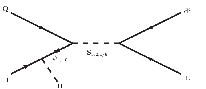
The contribution to $0\nu\beta\beta$ decay can be read off directly from the diagram in Fig. 1 on the left. It is given by

\displaystyle\frac{G_{F}\epsilon_{{\cal O}_{3,\#4}}}{\sqrt{2}}\simeq\frac{(Y_{\nu})_{e}v}{m_{\psi}}\frac{(Y_{d^{c}L})_{1e}(Y_{Q\psi})_{1}}{m_{S}^{2}}.

(7)

With only one copy of $\psi$ , the effective mass term contributing to $0\nu\beta\beta$ decay is $\langle m_{\nu}\rangle=(Y_{\nu})_{e}^{2}v^{2}/m_{\psi}$ and we can replace $(Y_{\nu})_{e}$ by $\langle m_{\nu}\rangle$ to arrive at the rough estimate of the constraint derived from the $d=7$ contribution to $0\nu\beta\beta$ :

(Y_{d^{c}L})_{1e}(Y_{Q\psi})_{1}\raise 1.29167pt\hbox{$\;<$\kern-7.5pt\raise-4.73611pt\hbox{$\sim\;$}}3\times 10^{-3}\left(\frac{\langle m_{\nu}\rangle}{\rm 0.5\hskip 2.84526pteV}\right)^{-1/2}\left(\frac{m_{\psi}}{\rm 100\hskip 2.84526ptGeV}\right)^{1/2}\left(\frac{m_{S}}{\rm 1\hskip 2.84526ptTeV}\right)^{2}

(8)

Eq. (8) shows that the upper limit on the Yukawa couplings disappears as $\langle m_{\nu}\rangle$ approaches zero. When the masses are greater than roughly $m_{\psi}\simeq m_{S}\sim 10$ TeV, the Yukawa couplings must be non-perturbative to fulfil the equality in Eq. (8). This implies that the mass mechanism will always dominate the $0\nu\beta\beta$ contribution for scales $\Lambda$ larger than roughly this value, independent of the exact choice of the couplings.

We briefly comment on models with more than one $\psi$ . As is well-known, neutrino oscillation data require at least two non-zero neutrino masses, while a model with only one $\psi$ leaves two of the three active neutrinos massless. Any realistic model based on Eq. (6) will therefore need at least two copies of $\psi$ . In this case Eq. (7) has to be modified to include the summation over the different $\psi_{i}$ and $\epsilon_{{\cal O}_{3,\#4}}\propto\sum_{i}\frac{(Y_{\nu})_{ei}v}{m_{\psi_{i}}}$ . $\langle m_{\nu}\rangle$ , on the other hand, is proportional to $\langle m_{\nu}\rangle\propto\sum_{i}\frac{(Y_{\nu})_{ei}^{2}}{m_{\psi_{i}}}$ . In this case, one still expects in general that limits derived from the long-range part of the amplitude are proportional to $\langle m_{\nu}\rangle$ . However, there is a special region in parameter space, where the different contributions to $\langle m_{\nu}\rangle$ cancel nearly exactly, leaving the long-range contribution being the dominant part of the amplitude. Unless the model parameters are fine-tuned in this way, the mass mechanism should win over the $d=7$ contribution for all tree-level neutrino mass models.

The tables in the appendix show, that all three types of seesaw mediators appear in the decompositions of ${\cal O}_{3}$ , ${\cal O}_{4}$ and ${\cal O}_{8}$ : $\psi_{1,1,0}$ (type-I), $\psi_{1,3,0}$ (type-III) and $S_{1,3,1}$ (type-II). In order to generate a seesaw mechanism, for some of the decompositions one needs to introduce new interactions, such as $S_{1,3,1}^{\dagger}HH$ , not present in the corresponding decomposition itself. However, in all these cases, the additional interactions are allowed by the symmetries of the models and are thus expected to be present. One then expects for all tree-level decompositions that the mass mechanism dominates over the long-range part of the amplitude, unless (i) the new physics scale $\Lambda$ is below a few TeV and (ii) some parameters are extremely fine-tuned to suppress light neutrino masses, as discussed above in our particular example decomposition.

III.2 One-loop level

We now turn to a discussion of one-loop neutrino mass models. For this class of neutrino mass models, naive estimates would put $\Lambda$ at $\Lambda\sim{\cal O}(10^{12})$ GeV for coefficients of ${\cal O}(1)$ and neutrino masses of $\mathcal{O}(0.1)$ eV. Thus, in the same way as tree neutrino mass models, the mass mechanism dominates over the long-range amplitude, unless at least some of the couplings in the UV completion are significantly smaller than ${\cal O}(1)$ , as discussed next.

As shown in [51], there are only three genuine 1-loop topologies for ( $d=5$ ) neutrino masses. Decompositions of ${\cal O}_{3}$ , ${\cal O}_{4}$ or ${\cal O}_{8}$ produce only two of them, namely T $\nu$ -I-ii or T $\nu$ -I-iii. We will discuss one example for T $\nu$ -I-ii, based on ${\cal O}_{3}$ decomposition $\#2$ , see Table 3 and Fig. 2. The underlying leptoquark model was first discussed in [52, 34], and for accelerator phenomenology see, e.g., [53]. The model adds two scalar states to the SM particle content, $S(3,1,-1/3)$ and $S^{\prime}(3,2,1/6)$ . The Lagrangian of the model contains interactions with SM fermions

{\cal L}_{3,\#2}^{\text{LQ}}=(\lambda_{S})_{\alpha i}{\overline{L_{\alpha}^{c}}}\cdot Q_{i}S^{\dagger}+(\lambda_{D})_{i\alpha}{\overline{d_{Ri}}}L_{\alpha}\cdot S^{\prime}+\cdots,

(9)

and the scalar interactions and mass terms:

{\cal L}_{3,\#2}^{\text{scalar}}=\mu SH\cdot S^{\prime\dagger}+m_{S}^{2}|S|^{2}+m_{D}^{2}|S^{\prime}|^{2}+\cdots

(10)

Lepton number is violated by the simultaneous presence of the terms in Eq. (9) and the first term in Eq. (10) [52]. Electro-weak symmetry breaking generates the off-diagonal element of the mass matrix for the scalars with the electric charge $-1/3$ . The mass matrix is expressed as

M^{2}_{\rm LQ}=\begin{pmatrix}m_{S}^{2}&\mu v\\ \mu v&m_{D}^{2}\end{pmatrix}

(11)

in the basis of ( $S^{-1/3},S^{\prime-1/3}$ ), which is diagonalized by the rotation matrix with the mixing angle $\theta_{\rm LQ}$ that is given as

\tan 2\theta_{\rm LQ}=\frac{2\mu v}{m_{S}^{2}-m_{D}^{2}}.

(12)

The neutrino mass matrix, which arises from the 1-loop diagram shown in Fig. 2, is calculated to be

(m_{\nu})_{\alpha\beta}=\frac{N_{c}\sin 2\theta_{\rm LQ}}{2(16\pi^{2})}\sum_{k}m_{d_{k}}\Delta B_{0}(m_{d_{k}}^{2},m_{1}^{2},m_{2}^{2})\Big\{(\lambda_{S})_{\alpha k}(\lambda_{D})_{k\beta}+(\alpha\leftrightarrow\beta)\Big\},

(13)

where $N_{c}=3$ is the colour factor. The loop-integral function $\Delta B_{0}$ is given as

\Delta B_{0}(m_{d_{k}}^{2},m_{1}^{2},m_{2}^{2})=\frac{m_{1}^{2}\ln(m_{1}^{2}/m_{d_{k}}^{2})}{m_{1}^{2}-m_{d_{k}}^{2}}-\frac{m_{2}^{2}\ln(m_{2}^{2}/m_{d_{k}}^{2})}{m_{2}^{2}-m_{d_{k}}^{2}}.

(14)

with the eigenvalues $m_{1,2}^{2}$ of the leptoquark mass matrix Eq. (11) and the mass $m_{d_{k}}$ of the down-type quark of the $k$ -th generation. Due to the hierarchy in the down-type quark masses, it is expected that the contribution from $m_{b}$ dominates the neutrino mass Eq. (13). For $m_{b}\ll{\bar{M}}$ and $\mu v\ll{\bar{M}}^{2}$ where ${\bar{M}}=m_{D}^{2}=m_{S}^{2}$ , Eq. (13) is reduced to

(m_{\nu})_{\alpha\beta}=\frac{3}{16\pi^{2}}\frac{\mu v}{{\bar{M}}^{2}}m_{b}\Big\{(\lambda_{S})_{\alpha 3}(\lambda_{D})_{3\beta}+(\alpha\leftrightarrow\beta)\Big\},

(15)

and this gives roughly

(\lambda_{S})_{e3}(\lambda_{D})_{3e}=10^{-2}\left(\frac{\langle m_{\nu}\rangle}{0.2{\rm eV}}\right)\left(\frac{\rm 1MeV}{\mu}\right)\left(\frac{{\bar{M}}}{\rm 1TeV}\right)^{2}.

(16)

The constraint on the effective neutrino mass $\langle m_{\nu}\rangle\lesssim 0.2$ eV is derived from the combined KamLAND-Zen and EXO data [41], which is $T_{1/2}\geq 3.4\times 10^{25}$ ys for ¹³⁶Xe. The same experimental results also constrain the coefficient of the $d=7$ operator generated from the Lagrangians Eqs. (9) and (10) as $\epsilon_{T_{R}}^{T_{R}}\raise 1.29167pt\hbox{$\;<$\kern-7.5pt\raise-4.73611pt\hbox{$\sim\;$}}5.6\times 10^{-10}$ (cf. Table 1), which gives

\displaystyle(\lambda_{S})_{e1}(\lambda_{D})_{1e}\lesssim

\displaystyle 3\cdot 10^{-2}\left(\frac{1{\rm MeV}}{\mu}\right)\left(\frac{\bar{M}}{1{\rm TeV}}\right)^{4}

(17)

Therefore, for $(\lambda_{S})_{e1}(\lambda_{D})_{1e}\simeq(\lambda_{S})_{e3}(\lambda_{D})_{3e}$ , the mass mechanism and the $d=7$ contribution are approximately of equal size with ${\bar{M}}\simeq 750$ GeV. Since $\langle m_{\nu}\rangle\propto{\bar{M}}^{-2}$ , while $\epsilon_{{\cal O}_{3,\#2}}\propto{\bar{M}}^{-4}$ , the mass mechanism will dominate $0\nu\beta\beta$ decay for ${\bar{M}}$ larger than ${\bar{M}}\simeq 750$ GeV, unless the couplings $(\lambda_{S})_{e1}(\lambda_{D})_{1e}$ are larger than $(\lambda_{S})_{e3}(\lambda_{D})_{3e}$ . We note that, leptoquark searches by the ATLAS [54, 55] and the CMS [56, 57, 58] collaborations have provided lower limits on the masses of the scalar leptoquarks, depending on the lepton generation they couple to and also on the decay branching ratios of the leptoquarks. The limits derived from the search for the pair-production of leptoquarks are roughly in the range $650-1000$ GeV [54, 55, 56, 57, 58], depending on assumptions.

The other 1-loop models are qualitatively similar to the example discussed above. However, the numerical values for masses and couplings in the high-energy completions should be different, depending on the Lorentz structure of the $d=7$ operators, see also the appendix.

III.3 Two-loop level

We now turn to a discussion of 2-loop neutrino mass models. As shown in the appendix, in case of the operators ${\cal O}_{3}$ and ${\cal O}_{4}$ , 2-loop models appear only for the cases ${\cal O}_{3a}$ and ${\cal O}_{4b}$ . As explained in section II, these operators alone cannot give realistic neutrino mass models. We thus base our example model on ${\cal O}_{8}$ . The 2-loop neutrino mass models based on ${\cal O}_{8}$ are listed in Tab. 5 in the appendix. In this section, we will discuss decomposition #15 in detail, which has not been discussed in the literature before.

In this model, we add the following states to the SM particle content:

	$\displaystyle(\psi_{L,R})_{3,2,7/6}=$	$\displaystyle\begin{pmatrix}\psi_{L,R}^{5/3}\\ \psi_{L,R}^{2/3}\end{pmatrix},$		(18)
	$\displaystyle(S_{3,2,1/6})_{k}=$	$\displaystyle\begin{pmatrix}S_{k}^{2/3}\\ S_{k}^{-1/3}\end{pmatrix}.$		(19)

With the new fields, we have the interactions

\displaystyle\mathcal{L}_{8,\#15}=

\displaystyle Y_{d_{i}L_{\alpha}S_{k}}\overline{d_{R,i}}L_{\alpha}\cdot S_{k}+Y_{u_{i}\psi H}\overline{u_{R,i}}\psi_{L}H^{\dagger}+Y_{e_{\alpha}\psi S_{k}}\overline{{e_{R\alpha}}^{c}}\psi_{R}S_{k}^{\dagger}+{\rm h.c.},

(20)

which mediate ${\cal O}_{8}$ operator, as shown in the left diagram of Fig. 3. Here, $i$ runs over the three quark generations. While $Y_{d_{i}L_{\alpha}S_{k}}$ and $Y_{u_{i}\psi H}$ could be different for different $i$ , for simplicity we will assume the couplings to quarks are the same for all $i$ and drop the index $i$ in the following. We will comment below, when we discuss the numerical results, on how this choice affects phenomenology. For simplicity, we introduce only one generation of the new fermion $\psi$ , while we allow for more than one copy of the scalar $S_{3,2,1/6}$ . Note that, in principle, the model would work also for one copy of $S_{3,2,1/6}$ and more than one $\psi$ , but as we will see later, the fit to neutrino data becomes simpler in our setup.

The fermion $\psi^{2/3}$ mixes with the up-type quarks through the following mass term:

	$\displaystyle{\cal L}_{\text{mass}}=$	$\displaystyle Y_{u}\langle H^{0}\rangle\overline{u_{L}}u_{R}+M_{\psi}\overline{\psi^{2/3}_{L}}\psi_{R}^{2/3}+Y_{u\psi H}^{\dagger}\langle H^{0}\rangle\overline{\psi_{L}^{2/3}}u_{R}+{\rm h.c.},$		(21)
	$\displaystyle=$	$\displaystyle\begin{pmatrix}\overline{t_{L}}&\overline{\psi_{L}^{2/3}}\end{pmatrix}\begin{pmatrix}m_{t}&0\\ \Delta&M_{\psi}\end{pmatrix}\begin{pmatrix}t_{R}\\ \psi_{R}^{2/3}\end{pmatrix}+{\rm h.c.},$

where $\Delta\equiv Y_{u\psi H}^{\dagger}\langle H^{0}\rangle$ .

Due to the strong hierarchy in up-type quark masses, we have assumed the sub-matrix for the up-type quarks in Eq. (21) is completely dominated by the contribution from top quarks. The mass matrix Eq. (21) is diagonalized with the unitary matrices $V_{L}$ and $V_{R}$ as

\displaystyle V_{L}^{\dagger}\begin{pmatrix}m_{t}&0\\ \Delta&M_{\psi}\end{pmatrix}V_{R}=\text{diag}({M}_{\Psi_{i}}),

(22)

and the mass eigenstates $\Psi^{2/3}_{i}$ are give as

\displaystyle\begin{pmatrix}t_{L}\\ \psi^{2/3}_{L}\end{pmatrix}_{a}=(V_{L})_{ai}\Psi^{2/3}_{Li}\quad\text{and}\quad\begin{pmatrix}t_{R}\\ \psi^{2/3}_{R}\end{pmatrix}_{a}=(V_{R})_{ai}\Psi^{2/3}_{Ri},

(23)

where the index $a$ for the interaction basis takes $a\in\{t,\psi\}$ . The interactions are written in the mass eigenbasis as follows:

	$\displaystyle{\cal L}_{W}=$	$\displaystyle\frac{g}{\sqrt{2}}{(V_{L}^{\dagger})_{it}}\overline{\Psi^{2/3}_{i}}\gamma^{\rho}P_{L}bW^{+}_{\rho}+{\rm h.c.},$		(24)
	$\displaystyle{\cal L}_{S}=$	$\displaystyle Y_{dL_{\alpha}S_{k}}\overline{d_{R}}L_{\alpha}\epsilon S_{k}+Y_{e_{\alpha}\psi S_{k}}(V_{R})_{\psi i}\overline{{e_{\alpha}}^{c}}P_{R}\Psi^{2/3}_{i}S_{k}^{-1/3{\dagger}}+Y_{e_{\alpha}\psi S_{k}}\overline{{e_{\alpha}}^{c}}P_{R}\psi^{5/3}S_{k}^{2/3{\dagger}}+{\rm h.c.}.$		(25)

The 2-loop neutrino mass diagram generated by this model is shown in Fig. 3. Using the formulas given in [59], one can express the neutrino mass matrix as

\displaystyle(m_{\nu})_{\alpha\beta}

\displaystyle=

\displaystyle\frac{N_{c}g^{2}m_{b}(V^{\dagger}_{L})_{it}(V_{R})_{\psi i}}{2(16\pi^{2})^{2}\ {M}_{\Psi_{i}}}\left[m_{e_{\alpha}}Y_{dL_{\beta}S_{k}}Y_{e_{\alpha}\psi S_{k}}+m_{e_{\beta}}Y_{dL_{\alpha}S_{k}}Y_{e_{\beta}\psi S_{k}}\right]I(z_{k,i},r_{i},t_{i}).

(26)

Here $N_{c}=3$ is the colour factor and $I(z_{k,i},r_{i},t_{i})$ is the loop integral defined as

\displaystyle I(z_{k,i},r_{i},t_{i})=\left[4{\hat{I}}(z_{k,i},r_{i},t_{i})-\frac{1}{t_{i}}{\hat{I}^{(k^{2})}}(z_{k,i},r_{i},t_{i})\right],

(27)

with

	$\displaystyle{\hat{I}}(z_{k,i},r_{i},t_{i})=\frac{1}{\pi^{4}}\int d^{4}q\int d^{4}k\frac{1}{(q^{2}-z_{k,i})(q^{2}-r_{i})(k^{2}-t_{i})k^{2}((q+k)^{2}-1)},$		(28)
	$\displaystyle{\hat{I}^{(k^{2})}}(z_{k,i},r_{i},t_{i})=\frac{1}{\pi^{4}}\int d^{4}q\int d^{4}k\frac{k^{2}}{(q^{2}-z_{k,i})(q^{2}-r_{i})(k^{2}-t_{i})k^{2}((q+k)^{2}-1)},$		(29)

The dimensionless parameters $z_{k,i},r_{i},t_{i}$ are defined as

\displaystyle z_{k,i}\equiv\frac{m^{2}_{S_{k}}}{M^{2}_{\Psi_{i}}},\quad\quad r_{i}\equiv\frac{m_{b}^{2}}{M^{2}_{\Psi_{i}}},\quad\quad\mathrm{and}\quad\quad t_{i}\equiv\frac{M^{2}_{W}}{M^{2}_{\Psi_{i}}}

(30)

and loop momenta $q$ and $k$ are also defined dimensionless. Due to the strong hierarchy in down-type quark masses, we expect that neutrino mass given in Eq. (26) is dominated by the contribution from bottom quark. If we assume in Eq. (26) that all Yukawa couplings are of the same order, then the entries of the neutrino mass matrix will have a strong hierarchy: $(m_{\nu})_{ee}:(m_{\nu})_{\mu\mu}:(m_{\nu})_{\tau\tau}=m_{e}:m_{\mu}:m_{\tau}$ . Such a flavor structure is not consistent with neutrino oscillation data. Therefore, in order to reproduce the observed neutrino masses and mixings, our Yukawa couplings need to have a certain compensative hierarchy in their flavor structure.

Since the neutrino mass matrix, and thus the Yukawa couplings contained in the neutrino mass, have a non-trivial flavour pattern, these Yukawas will be also constrained by charged lepton flavour violation (LFV) searches. Here we discuss only $\mu\to e\gamma$ which usually provides the most stringent constraints in many models. In order to calculate the process $\mu\rightarrow e\gamma$ we adapt the general formulas shown in [60] for our particular case. The amplitude for $\mu\rightarrow e\gamma$ decay is given by

\displaystyle{\cal{M}}(\mu\rightarrow e\gamma)=e\epsilon^{*}_{\alpha}q_{\beta}\bar{u}(p_{e})i\sigma^{\alpha\beta}(\sigma_{R}P_{R}+\sigma_{L}P_{L})u(p_{\mu}).

(31)

Here, $\epsilon_{\alpha}$ is the photon polarization vector and $q_{\beta}$ is the momentum of photon. Three different diagrams contribute to the amplitude for $\mu\rightarrow e\gamma$ , which are finally summarized with the two coefficients $\sigma_{R}$ and $\sigma_{L}$ given by

\displaystyle\sigma_{R}=i\frac{m_{\mu}}{16\pi^{2}}\left[Y_{dL_{2}S_{k}}^{\dagger}Y_{dL_{1}S_{k}}\frac{2F_{2}(x_{b,k})-F_{1}(x_{b,k})}{m_{S_{k}}^{2}}\right],

(32)

\displaystyle\sigma_{L}=i\frac{m_{\mu}}{16\pi^{2}}\left[Y^{\dagger}_{e_{2}\psi S_{k}}Y_{e_{1}\psi S_{k}}\frac{-F_{2}(x_{\psi,k})-7F_{1}(x_{\psi,k})}{m_{S_{k}}^{2}}\right],

(33)

where $x_{\psi,k}\equiv\frac{M^{2}_{\psi}}{m^{2}_{S_{k}}}$ and $x_{b,k}\equiv\frac{m^{2}_{b}}{m^{2}_{S_{k}}}$ . Here, we have assumed that both the $\psi^{-2/3}$ and the $\psi^{-5/3}$ have the same mass $M_{\psi}$ . This neglects (small) mass shifts in the $\psi^{-2/3}$ state, due to its mixing with the top quark. Due to the large value of $M_{\psi}$ , that we use in our numerical examples, this should be a good approximation. Note also, that the contribution from the top quark is negligible for those large values of $M_{\psi}$ used below. The functions $F_{1}(x)$ and $F_{2}(x)$ are defined in Eqs (40) and (41) in [60] as

	$\displaystyle F_{1}(x)=$	$\displaystyle\frac{x^{2}-5x-2}{12(x-1)^{3}}+\frac{x\ln x}{2(x-1)^{4}},$		(34)
	$\displaystyle F_{2}(x)=$	$\displaystyle\frac{2x^{2}+5x-1}{12(x-1)^{3}}-\frac{x^{2}\ln x}{2(x-1)^{4}},$		(35)

The branching ratio for $\mu\rightarrow e\gamma$ can be expressed with the coefficients $\sigma_{R}$ and $\sigma_{L}$ as

\displaystyle\mathrm{Br}(\mu\rightarrow e\gamma)=\frac{e^{2}m_{\mu}^{3}(\left|\sigma_{R}\right|^{2}+\left|\sigma_{L}\right|^{2})}{16\pi\ \Gamma_{\mu}},

(36)

where $\Gamma_{\mu}$ is the total decay width of muon. Later, we will numerically calculate the branching ratio to search for the parameter choices that are consistent with the oscillation data and the constraint from $\mu\rightarrow e\gamma$ .

Before discussing constraints from lepton flavour violation, we will compare the long-range contribution to $0\nu\beta\beta$ with the mass mechanism in this model. This model manifestly generates a $d=7$ long-range contribution to $0\nu\beta\beta$ . The half-life of $0\nu\beta\beta$ induced by the long-range contribution is proportional to the coefficient $\epsilon_{V+A}^{V+A}$ which is expressed in terms of the model parameters as

\displaystyle\epsilon_{V+A}^{V+A}=\frac{\sqrt{2}}{G_{F}}\frac{\Delta}{M_{\psi}}\frac{Y_{e_{1}\psi S_{k}}Y_{dL_{1}S_{k}}}{2m_{S_{k}}^{2}}\raise 1.29167pt\hbox{$\;<$\kern-7.5pt\raise-4.73611pt\hbox{$\sim\;$}}3.9\times 10^{-7}.

(37)

Here, we use the limit on $\epsilon_{V+A}^{V+A}$ from non-observation of ¹³⁶Xe $0\nu\beta\beta$ decay, see Table 1. With one copy of the new scalar, the bound of Eq. (37) is directly related to the effective neutrino mass Eq. (26) and places the stringent constraint:

\displaystyle\langle m_{\nu}\rangle\lesssim 2\times 10^{-5}\text{[eV]}\left(\frac{m_{S}}{10\text{[TeV]}}\right)^{2}\left(\frac{I(z_{k,1},r_{1},t_{1})}{5\times 10^{-2}}\right),

(38)

where we have used the approximate relation

\displaystyle\frac{(V^{\dagger}_{L})_{it}(V_{R})_{\psi i}I(z_{k,i},r_{i},t_{i})}{{M}_{\Psi_{i}}}\simeq\frac{I(z_{k,1},r_{1},t_{1})\Delta}{M_{\psi}m_{t}},

(39)

with $z_{k,1}=(m_{S_{k}}/m_{t})^{2}$ , $r_{1}=(m_{b}/m_{t})^{2}$ , $t_{1}=(M_{W}/m_{t})^{2}$ , and $I(z_{k,1},r_{1},t_{1})\sim 5\times 10^{-2}$ for a scalar mass of $m_{S}=10$ TeV and $M_{\psi}\simeq 0.8$ TeV. Note that this parameter choice is motivated by the fact that the model cannot fit neutrino data with perturbative Yukawa couplings with scalar masses larger than $m_{S}\raise 1.29167pt\hbox{$\;>$\kern-7.5pt\raise-4.73611pt\hbox{$\sim\;$}}10$ TeV. As one can see from Eq. (38), the long-range contribution to $0\nu\beta\beta$ clearly dominates over the mass mechanism in this setup.

In short, this neutrino mass model predicts large decay rate of $0\nu\beta\beta$ but tiny $\langle m_{\nu}\rangle$ . This implies that, if future neutrino oscillation experiments determine that the neutrino mass pattern has normal hierarchy but $0\nu\beta\beta$ is discovered in the next round of experiments, the $0\nu\beta\beta$ decay rate is dominated by the long-range part of the amplitude. Recall that ${\cal O}_{8}$ contains $\overline{e^{c}}$ . This implies that the model predicts a different angular distribution than the mass mechanism, which in principle could be tested in an experiment such as Super-NEMO [61].

Note that, to satisfy the condition Eq. (38), cancellations among different contributions to $\langle m_{\nu}\rangle$ are necessary. This can be arranged only if we consider at least two generations of the new particles in the model (either the scalar $S$ or the fermion $\psi$ ).

Here we discuss more on the consistency of our model with the neutrino masses and mixings observed at the oscillation experiments. Instead of scanning whole the parameter space, we illustrate the parameter choice that reproduces the neutrino properties and is simultaneously consistent with the bound from lepton flavour violation. To simplify the discussion we use the following ansatz in the flavour structure of the Yukawa couplings:

Y_{dL_{\alpha}S_{k}}=\frac{Y_{e_{\alpha}\psi S_{k}}}{y}\frac{m_{e_{\alpha}}}{m_{\mu}}

(40)

with a dimensionless parameter $y$ . With Eq. (40), the neutrino mass matrix Eq. (26) is reduced to

\displaystyle(m_{\nu})_{\alpha\beta}=(\Lambda)_{\alpha k}\mathcal{I}_{k}(\Lambda^{T})_{k\beta},

(41)

where $\Lambda$ is defined as

\displaystyle\Lambda_{\alpha k}\equiv Y_{dL_{\alpha}S_{k}}=\frac{Y_{e_{\alpha}\psi S_{k}}}{y}\frac{m_{e_{\alpha}}}{m_{\mu}},

(42)

and $\mathcal{I}$ is given as

\displaystyle\mathcal{I}_{k}=\frac{N_{c}g^{2}ym_{b}m_{\mu}(V^{\dagger}_{L})_{it}(V_{R})_{\psi i}}{(16\pi^{2})^{2}M_{\Psi_{i}}}I(z_{k,i},r_{i},t_{i}).

(43)

We introduce three copies of the new scalar $S^{-1/3}_{k}$ . The resulting mass matrix Eq. (41) has the same index structure as that of the type-I seesaw mechanism, and therefore, the matrix $\Lambda$ can be expressed as

\displaystyle\left(\Lambda^{T}\right)_{k\alpha}=\left(\sqrt{\mathcal{I}^{-1}}\right)_{k}R_{ki}\left(\sqrt{\hat{m}_{\nu}}\right)_{i}\left(U_{\nu}^{\dagger}\right)_{i\alpha},

(44)

following the parameterization developed by Casas and Ibarra [62].

Here, $\hat{m}_{\nu}$ is the neutrino mass matrix in the mass eigenbasis, and the mass matrix $m_{\nu}$ is diagonalized with the lepton mixing matrix $U_{\nu}$ as

(\hat{m}_{\nu})_{i}\equiv\text{diag}\begin{pmatrix}m_{\nu_{1}}&m_{\nu_{2}}&m_{\nu_{3}}\end{pmatrix}=(U_{\nu}^{T})_{i\alpha}\,(m_{\nu})_{\alpha\beta}\,(U_{\nu})_{\beta j}

(45)

for which we use the following standard parametrization

U_{\nu}=\left(\begin{array}[]{ccc}c_{12}c_{13}&s_{12}c_{13}&s_{13}e^{i\delta}\\ -s_{12}c_{23}-c_{12}s_{23}s_{13}e^{-i\delta}&c_{12}c_{23}-s_{12}s_{23}s_{13}e^{-i\delta}&s_{23}c_{13}\\ s_{12}s_{23}-c_{12}c_{23}s_{13}e^{-i\delta}&-c_{12}s_{23}-s_{12}c_{23}s_{13}e^{-i\delta}&c_{23}c_{13}\end{array}\right)\left(\begin{array}[]{ccc}1&0&0\\ 0&e^{i\alpha_{21}}&0\\ 0&0&e^{i\alpha_{31}}\end{array}\right).

(46)

Here $c_{ij}=\cos\theta_{ij}$ , $s_{ij}=\sin\theta_{ij}$ with the mixing angles $\theta_{ij}$ , $\delta$ is the Dirac phase and $\alpha_{21}$ , $\alpha_{31}$ are Majorana phases. The matrix $R$ is a complex orthogonal matrix which can be parametrized in terms of three complex angles as

R\ =\ \left(\begin{array}[]{ccc}c_{2}c_{3}&-c_{1}s_{3}-s_{1}s_{2}c_{3}&s_{1}s_{3}-c_{1}s_{2}c_{3}\\ c_{2}s_{3}&c_{1}c_{3}-s_{1}s_{2}s_{3}&-s_{1}c_{3}-c_{1}s_{2}s_{3}\\ s_{2}&s_{1}c_{2}&c_{1}c_{2}\end{array}\right).

(47)

Note that it is assumed in this procedure that the charged lepton mass matrix is diagonal. After fitting the neutrino oscillation data with the parametrization shown above, there remain $y$ , $Y_{u\psi H}$ and the masses $M_{\psi}$ , $m_{S_{k}}$ for $k=1,2,3$ as free parameters. For simplicity, we assume a degenerate spectrum of the heavy scalars $m_{S}=m_{S_{k}}$ .

In Fig. 4-(a), we plot the half-life $T_{1/2}^{0\nu\beta\beta}$ as a function of $m_{\nu_{1}}$ for fixed values of the coupling $Y_{u\psi H}=0.6$ and the masses $M_{\psi}=800\ \text{GeV}$ and $m_{S}=10$ TeV. The parameter $y$ is taken to be $10^{-3}$ , since this minimizes the decay rate of $\mu\rightarrow e\gamma$ , as we will discuss below. We have used oscillation parameters for the case of normal hierarchy. The region enclosed by the red curves is $d=7$ long-range contribution to $0\nu\beta\beta$ , and the blue curves correspond to the mass mechanism contribution only, which is shown for comparison. The gray region is already excluded by $0\nu\beta\beta$ searches, and for the model under consideration only the cyan region is allowed. As one can see from Fig. 4-(a), the total contribution to $0\nu\beta\beta$ is dominated by the $d=7$ long-range contribution. Note that the mass mechanism and the long-range contribution are strictly related only under the assumption that $Y_{u\psi H}$ and $Y_{dL_{\alpha}S_{k}}$ are independent of the quark generation $i$ . This is so, because the 2-loop diagram is dominated by 3rd generation quarks, while in $0\nu\beta\beta$ decay only first generation quarks participate. If we were to drop this assumption and put the first generation couplings to $Y_{u_{1}\psi H}\raise 1.29167pt\hbox{$\;<$\kern-7.5pt\raise-4.73611pt\hbox{$\sim\;$}}10^{-2}\times Y_{u_{3}\psi H}$ and $Y_{d_{1}L_{\alpha}S_{k}}\raise 1.29167pt\hbox{$\;<$\kern-7.5pt\raise-4.73611pt\hbox{$\sim\;$}}10^{-2}\times Y_{d_{3}L_{\alpha}S_{k}}$ , the half-life for the long-range amplitude would become comparable to the mass mechanism, without changing the fit to oscillation data.

Note that non-zero Majorana phases are necessary to allow for cancellations among the mass mechanism contributions, so as to make $\langle m_{\nu}\rangle$ small as required by Eq. (38). In Fig. 4-(b), we plot the half-life $T_{1/2}^{0\nu\beta\beta}$ as a function of the scalar mass $m_{S}$ . Here we fixed the oscillation parameters to $m_{\nu_{1}}=1.23\times 10^{-3}$ eV , $\alpha_{21}=0$ , $\alpha_{31}=\pi/2$ , $s_{23}^{2}=1/2$ and $s_{12}^{2}=1/3$ and the remaining oscillation parameters $\Delta m_{31}^{2}$ and $\Delta m_{21}^{2}$ to their best-fit values for the case of normal hierarchy. The plot assumes that the matrix $R$ is equal to the identity. The plot shows that the half-life increases to reach approximately $T_{1/2}^{0\nu\beta\beta}\sim 10^{26}$ yr for $m_{S}=10$ TeV.

Now we discuss the constraint from lepton flavour violating process $\mu\to e\gamma$ . In Fig. 5, we show Br( $\mu\to e\gamma$ ) as a function of the scalar $m_{S}$ and the parameter $y$ for fixed values of the coupling $Y_{u\psi H}=0.6$ and the fermion mass $M_{\psi}=800\ \text{GeV}$ , which is the same parameter choice adopted in Fig. 4. These plots show that the current experimental limits on Br( $\mu\to e\gamma$ ) put strong constraints on the model under consideration. In Fig. 5-(a), we plot Br $(\mu\rightarrow e\gamma)$ with different values of the parameter $y=\{10^{-1},10^{-2},10^{-3}\}$ . We have used again the parameters $m_{\nu_{1}}=1.23\times 10^{-3}$ eV, $\alpha_{21}=0$ , $\alpha_{31}=\pi/2$ , $s_{23}^{2}=1/2$ and $s_{12}^{2}=1/3$ fixing the remaining oscillation parameters $\Delta m_{31}^{2}$ and $\Delta m_{21}^{2}$ at their best-fit values for the case of normal hierarchy. With the choice of $y=10^{-1}$ , the entire region of $m_{S}$ is not consistent with the current experimental limits. On the other hand, we can easily avoid the constraint from $\mu\rightarrow e\gamma$ by setting the parameter $y$ to be roughly smaller than $10^{-2}$ . Note that the curves with $y=10^{-1}$ and $y=10^{-3}$ do not cover the full range of $m_{S}$ . This is because the fit to neutrino data would require Yukawa couplings in the perturbative regime. (We define the boundary to perturbativity as at least one entry in the Yukawa matrix being smaller than $\sqrt{4\pi}$ .) It is necessary to have smaller values of the parameter $y$ to obey the experimental bound. This feature is also shown in Fig. 5-(b) where we plot the Br( $\mu\to e\gamma$ ) as a function of $y$ with different values of the mass $m_{S}=\{1,5,10\}$ TeV. As shown, for $y\lesssim 10^{-2}$ it is possible to fulfil the experimental limit, having the Br( $\mu\to e\gamma$ ) a minimum around $y=10^{-3}$ . Because of the perturvative condition, the curves with $m_{S}=5$ TeV and $m_{S}=10$ TeV end in the middle of the $y$ space. The reason for the strong dependence of Br( $\mu\to e\gamma$ ) on the parameter $y$ can be understood as follows: As shown in Eq. (42) the Yukawa couplings $Y_{dL_{\alpha}S_{k}}$ and $Y_{e_{\alpha}\psi S_{k}}$ are related in the neutrino mass fit, but only up to an overall constant, $\frac{1}{y}$ . For values of $y$ of the order of $10^{-3}$ both Yukawas are of the same order and this minimizes Br( $\mu\to e\gamma$ ). If $y$ is much larger (much smaller) than this value $Y_{dL_{\alpha}S_{k}}$ ( $Y_{e_{\alpha}\psi S_{k}}$ ) becomes much larger than $Y_{e_{\alpha}\psi S_{k}}$ ( $Y_{dL_{\alpha}S_{k}}$ ) and since the different diagrams contributing to Br( $\mu\to e\gamma$ ) are proportional to the individual Yukawas (and not their product) this leads to a much larger rate for Br( $\mu\to e\gamma$ ).

In summary, for all 2-loop $d=7$ models of neutrino mass, which lead to ${\cal O}_{8}$ , the long-range part of the amplitude will dominate over the mass mechanism by a large factor, unless there is a strong hierarchy between the non-SM Yukawa couplings to the first and third generation quarks. Such models are severely constrained by lepton flavour violation and $0\nu\beta\beta$ decay. We note again, that these models predict an angular correlation among the out-going electrons which is different from the mass mechanism.

IV Left-right symmetric model: $d=7$ versus $d=9$ operator

Writing new physics contributions to the SM in a series of NROs assumes implicitly that higher order operators are suppressed with respect to lower order ones by additional inverse powers of the new physics scale $\Lambda$ . However, there are some particular example decompositions for (formally) higher-order operators, where this naive power counting fails. We will discuss again one particular example in more detail. The example we choose describes the situation encountered in left-right symmetric extensions of the standard model.

Consider the following two Babu-Leung operators:

\displaystyle{\cal O}_{8}=L^{i}\overline{e^{c}}\hskip 1.42271pt\overline{u^{c}}d^{c}H^{j}\epsilon_{ij}

\displaystyle{\cal O}_{7}=L^{i}Q^{j}\overline{e^{c}}\overline{Q}_{k}H^{k}H^{l}H^{m}\epsilon_{il}\epsilon_{jm}

(48)

${\cal O}_{8}$ can be decomposed in a variety of ways, decomposition #14 (see Table 5) is shown in Fig. 6 to the left. The charged vector appearing in this diagram couples to a pair of right-handed quarks and, thus, can be interpreted as the charged component of the adjoint of the left-right symmetric (LR) extension of the SM, based on the gauge group $SU(3)_{C}\times SU(2)_{L}\times SU(2)_{R}\times U(1)_{B-L}$ . In LR right-handed quarks are doublets, $Q^{c}=\Psi_{\bar{3},1,2,-1/6}$ , the $\psi_{1,1,0}$ can be understood as the neutral member of $L^{c}$ , i.e. the right-handed neutrino, and the Higgs doublet is put into the bidoublet, $\Phi_{1,2,2,0}$ . The resulting diagram for $0\nu\beta\beta$ decay is shown in Fig. 6 on the right.

Fig. 6 gives a long-range contribution to $0\nu\beta\beta$ decay. We can estimate the size of $\epsilon_{{\cal O}_{8}}$ from these diagrams:

\displaystyle\frac{G_{F}\epsilon_{{\cal O}_{8,\#14}}}{\sqrt{2}}=\frac{Y_{L\psi}g_{1}g_{2}v_{\rm SM}}{m_{V}^{2}m_{\psi}}=\frac{Y_{LL^{c}}g_{R}^{2}v_{u}}{m_{W_{R}}^{2}m_{\nu_{R}}}

(49)

The first of these two equations shows $\epsilon_{{\cal O}_{8}}$ for Fig. 6 on the left (notation for SM gauge group), the second for Fig. 6 on the right (notation for gauge group of the LR model). Here, $g_{1}$ and $g_{2}$ could be different, in principle, but are equal to $g_{R}$ in the LR model. $v_{\rm SM}$ is the SM vev, fixed by the $W$ -mass. In the LR model, the bi-doublet(s) contain in general two vevs. We call them $v_{d}$ and $v_{u}$ here and $v_{\rm SM}^{2}=v_{d}^{2}+v_{u}^{2}$ . In Eq. (49) only $v_{u}=v_{\rm SM}\sin\beta$ , with $\tan\beta=v_{u}/v_{d}$ , appears. Note that we have suppressed again generation indices and summations in Eq. (49). We will come back to this important point below.

Now, however, first consider ${\cal O}_{7}$ . From the many different possible decompositions we concentrate on the one shown in Fig. 7. The diagram on the left shows the diagram in SM notation, the diagram on the right is the corresponding LR embedding. It is straightforward to estimate the size of these diagrams as:

\displaystyle\frac{G_{F}\epsilon_{{\cal O}_{7}}}{\sqrt{2}}=\frac{Y_{L\psi}g_{1}g_{2}g_{3}^{2}v_{\rm SM}^{3}}{m_{V_{1,3,0}}^{2}m_{V_{1,1,1}}^{2}m_{\psi}}=\frac{Y_{LL^{c}}g_{L}^{2}g_{R}^{2}v_{u}^{2}v_{d}}{m_{W_{R}}^{2}m_{W_{L}}^{2}m_{\nu_{R}}}\propto\frac{Y_{LL^{c}}g_{R}^{2}v_{u}}{m_{W_{R}}^{2}m_{\nu_{R}}}

(50)

Arbitrarily we have called the 4-point coupling in the left diagram $g_{3}^{2}$ . In the LR model again the couplings are fixed to $g_{L}$ and $g_{R}$ . In the last relation in Eq. (50) we have used $v_{\rm SM}^{2}\propto m_{W_{L}}^{2}/g_{L}^{2}$ . This shows that Eq. (50) is of the same order than Eq. (49), despite coming from a $d=9$ operator. This a priori counter-intuitive result is a simple consequence of the decomposition containing the SM $W_{L}$ boson. Any higher-order operator which can be decomposed in such a way will behave similarly, i.e. $1/\Lambda^{5}\Rightarrow 1/(\Lambda^{3}v_{\rm SM}^{2})$ .⁸⁸ 8 In addition to the case of the SM W-boson, discussed here, similar arguments apply to decompositions containing the scalar $S_{1,2,1/2}$ , which can be interpreted as the SM Higgs boson.

We note that in this particular example the contribution of ${\cal O}_{7}$ is actually more stringently constrained than the one from ${\cal O}_{8}$ . This is because ${\cal O}_{8}$ leads to a low-energy current of the form ( $V+A$ ) in both, the leptonic and the hadronic indices, i.e. the limit corresponds to $\epsilon^{V+A}_{V+A}$ . ${\cal O}_{7}$ , on the other hand, leads to $\epsilon^{V+A}_{V-A}$ , which is much more tightly constraint due to contribution from the nuclear recoil matrix element [64], compare values in Table 1.

We note that, one can identify the diagrams in Fig. 6 and Fig. 7 with the terms proportional to $\lambda$ and $\eta$ in the notation of [64], used by many authors in $0\nu\beta\beta$ decay. For the complete expressions for the long-range part of the amplitude, one then has to sum over the light neutrino mass eigenstates, taking into account that the leptonic vertices in the diagrams in Figs. 6 and 7 are right-handed. Defining the mixing matrices for light and heavy neutrinos as $U_{\alpha j}$ and $V_{\alpha j}$ , respectively, as in [64], the coefficients $\epsilon_{{\cal O}_{8}}$ and $\epsilon_{{\cal O}_{7}}$ of the $d=7$ and $d=9$ operators are then the effective couplings [64]:

\displaystyle\langle\lambda\rangle=\sum_{j=1}^{3}U_{ej}V_{ej}\lambda

\displaystyle\langle\eta\rangle=\sum_{j=1}^{3}U_{ej}V_{ej}\eta.

(51)

Orthogonality of $U_{ej}$ and $V_{ej}$ leads to $\sum_{j=1}^{6}U_{ej}V_{ej}\equiv 0$ . However, the sum in Eq. (51) runs only over the light states, which does not vanish exactly, but rather is expected to be of the order of the light-heavy neutrino mixing. In left-right symmetric models with seesaw (type-I), one expects this mixing to be of order $m_{D}/M_{M}\sim\sqrt{m_{\nu}/M_{M}}$ , where $m_{D}$ is ( $M_{M}$ ) the Dirac mass (Majorana mass) for the (right-handed) neutrinos and $m_{\nu}$ is the light neutrino mass. This, in general, is expected to be a small number of order $\sum_{j=1}^{3}U_{ej}V_{ej}\sim 10^{-5}\sqrt{(\frac{m_{\nu}}{\rm 0.1eV})(\frac{\rm 1TeV}{M_{M}})}$ . In this case one expects the mass mechanism to dominate over both $\langle\lambda\rangle$ and $\langle\eta\rangle$ , given current limits on $W_{L}-W_{R}$ mixing [65] and lower limits on the $W_{R}$ mass from LHC [66, 67]. However, as in the LQ example model discussed previously in section III.1, contributions to the neutrino mass matrix contain a sum over the three heavy right-handed neutrinos. In the case of severe fine-tuning of the parameters entering the neutrino mass matrix, the connection between the light-heavy neutrino mixing and $\langle m_{\nu}\rangle$ can be avoided, see section III.1. In this particular part of parameter space, the incomplete $\sum_{j=1}^{3}U_{ej}V_{ej}$ could in principle be larger than the naive expectation. Recall that the current bound on non-unitarity of $U$ is of the order of 1 % [49]. For $\sum_{j=1}^{3}U_{ej}V_{ej}$ as large as $\sum_{j=1}^{3}U_{ej}V_{ej}\sim{\cal O}(10^{-2})$ $\langle\lambda\rangle$ and/or $\langle\eta\rangle$ could dominate over the mass mechanism, even after taking into account all other existing limits. We stress again that this is not the natural expectation.

In summary, there are some particular decompositions of $d=9$ operators containing the SM W or Higgs boson. In those cases the $d=9$ operator scales as $1/(\Lambda^{3}v_{\rm SM}^{2})$ and can be as important as the corresponding decomposition of the $d=7$ operator.

V Summary

We have studied $d=7$ $\Delta L=2$ operators and their relation with the long-range part of the amplitude for $0\nu\beta\beta$ decay. We have given the complete list of decompositions for the relevant operators and discussed a classification scheme for these decompositions based on the level of perturbation theory, at which the different models produce neutrino masses. For tree-level and 1-looop neutrino mass models we expect that the mass mechanism is more important than the long-range ( $p\hskip-5.0pt/\;\>$ -enhanced) amplitude. We have discussed how this conclusion may be avoided in highly fine-tuned regions in parameter space. For 2-loop neutrino mass models based on $d=7$ operators, the long-range amplitude usually is more important than the mass mechanism. To demonstrate this, we have discussed in some detail a model based on ${\cal O}_{8}$ .

We also discussed the connection of our work with previously considered long-range contributions in left-right symmetric models. This served to point out some particularities about the operator classification, that we rely on, in cases where higher order operators, such as $d=9$ ( ${\cal O}_{9}\propto\Lambda_{\rm LNV}^{-5}$ ), are effectively reduced to lower order operators, i.e. $d=7$ ( ${\cal O}_{9}^{\text{eff}}\propto\Lambda_{\rm LNV}^{-3}\times\Lambda_{\rm EW}^{-2}$ ).

Our main results are summarized in tabular form in the appendix, where we give the complete list of possible models, which lead to contributions to the long-range part of the amplitude for $0\nu\beta\beta$ decay. From this list one can deduce, which contractions can lead to interesting phenomenology, i.e. models that are testable also at the LHC.

Acknowledgements

M.H. thanks the Universidad Tecnica Federico Santa Maria, Valparaiso, for hospitality during his stay. M.H. is supported by the Spanish grants FPA2014-58183-P and Multidark CSD2009-00064 (MINECO), and PROMETEOII/2014/084 (Generalitat Valenciana). J.C.H. is supported by Fondecyt (Chile) under grants 11121557 and by CONICYT (Chile) project 791100017. The research of T.O. is supported by JSPS Grants-in-Aid for Scientific Research on Innovative Areas Unification and Development of the Neutrino Science Frontier Number 2610 5503.

VI Appendix

Here we present the summary tables of all tree-level decompositions of the Babu-Leung operators #3 (Tab. 3), #4 (Tab. 4), and #8 (Tab. 5) with mass dimension $d=7$ . The effective operators are decomposed into renormalizable interactions by assigning the fields to the outer legs of the tree diagram shown in Fig. 8.

The assignments of the outer fields are shown at the “Decompositions” column, and the (inner) fields required by the corresponding decompositions are listed at the “Mediators” column. The symbols $S$ and $\psi$ represents the Lorentz nature of the mediators: $S^{(^{\prime})}$ is a scalar field, and $\psi_{L(R)}$ is a left(right)-handed fermion. The charges of the mediators under the SM gauge groups are identified and expressed with the format $(SU(3)_{c},SU(2)_{L})_{U(1)_{Y}}$ . It is easy to find the contributions of the effective operators to neutrinoless double beta decay processes at the “Projection to the basis ops.” column. The basis operators are defined as

$\displaystyle\mathcal{O}_{3a}(\alpha,\beta)\equiv$	$\displaystyle({\rm i}\tau^{2})^{ij}({\rm i}\tau^{2})^{kl}\{(\overline{L^{c}}_{\alpha})_{i}^{a}(L_{\beta})_{ja}\}\{(\overline{d_{R}})^{Ib}(Q)_{Ikb}\}H_{l}$
$\displaystyle\supset$	$\displaystyle\frac{1}{4}\left[j_{S+P}^{\dagger}(\alpha,\beta)-j_{S+P}^{\dagger}(\beta,\alpha)\right]J_{S+P}^{\dagger}H^{0},\allowbreak$	(52)
$\displaystyle\mathcal{O}_{3b}(\alpha,\beta)\equiv$	$\displaystyle({\rm i}\tau^{2})^{ik}({\rm i}\tau^{2})^{jl}\{(\overline{L^{c}}_{\alpha})_{i}^{a}(L_{\beta})_{ja}\}\{(\overline{d_{R}})^{Ib}(Q)_{Ikb}\}H_{l}$
$\displaystyle\supset$	$\displaystyle-\frac{1}{4}j_{S+P}^{\dagger}(\beta,\alpha)J_{S+P}^{\dagger}H^{0}+\frac{1}{4}\{\overline{\ell^{c}}_{\alpha}(1-\gamma^{5})\ell_{\beta}\}J_{S+P}^{\dagger}H^{+},\allowbreak$	(53)
$\displaystyle\mathcal{O}_{3a}^{\text{ten.}}(\alpha,\beta)\equiv$	$\displaystyle({\rm i}\tau^{2})^{ij}({\rm i}\tau^{2})^{kl}\{(\overline{L^{c}}_{\alpha})_{i}^{a}{(\sigma^{\rho\sigma})_{a}}^{b}(L_{\beta})_{jb}\}\{(\overline{d_{R}})^{Ic}{(\sigma_{\rho\sigma})_{c}}^{d}(Q)_{Ikd}\}H_{l}$
$\displaystyle\supset$	$\displaystyle-\frac{1}{16}\left[(j_{T_{R}}^{\dagger})^{\rho\sigma}(\alpha,\beta)+(j_{T_{R}}^{\dagger})^{\rho\sigma}(\beta,\alpha)\right](J_{T_{R}}^{\dagger})_{\rho\sigma}H^{0},\allowbreak$	(54)
$\displaystyle\mathcal{O}_{3b}^{\text{ten.}}(\alpha,\beta)\equiv$	$\displaystyle({\rm i}\tau^{2})^{ik}({\rm i}\tau^{2})^{jl}\{(\overline{L^{c}}_{\alpha})_{i}^{a}{(\sigma^{\rho\sigma})_{a}}^{b}(L_{\beta})_{jb}\}\{(\overline{d_{R}})^{Ic}{(\sigma_{\rho\sigma})_{c}}^{d}(Q)_{Ikd}\}H_{l}$
$\displaystyle\supset$	$\displaystyle-\frac{1}{16}(j_{T_{R}}^{\dagger})^{\rho\sigma}(\beta,\alpha)(J_{T_{R}}^{\dagger})_{\rho\sigma}H^{0}-\frac{1}{16}\{\overline{{\ell}^{c}}_{\alpha}\gamma^{\rho\sigma}(1-\gamma^{5})\ell_{\beta}\}(J_{T_{R}}^{\dagger})_{\rho\sigma}H^{+},\allowbreak$	(55)
$\displaystyle\mathcal{O}_{4a}(\alpha,\beta)\equiv$	$\displaystyle({\rm i}\tau)^{jk}(\overline{L^{c}}_{\alpha})_{i}^{a}(L_{\beta})_{ja}(\overline{Q})^{Ii}_{\dot{a}}(u_{R})_{I}^{\dot{a}}H_{k}$
$\displaystyle\supset$	$\displaystyle\frac{1}{4}j_{S+P}^{\dagger}(\beta,\alpha)J_{S-P}^{\dagger}H^{0}-\frac{1}{4}\overline{\ell^{c}}_{\alpha}(1-\gamma^{5})\ell_{\beta}J_{S-P}^{\dagger}H^{+},\allowbreak$	(56)
$\displaystyle\mathcal{O}_{4b}(\alpha,\beta)\equiv$	$\displaystyle({\rm i}\tau^{2})^{ij}(\overline{L^{c}}_{\alpha})_{i}^{a}(L_{\beta})_{ja}(\overline{Q})^{Ik}_{\dot{a}}(u_{R})_{I}^{\dot{a}}H_{k}$
$\displaystyle\supset$	$\displaystyle\frac{1}{4}\left[j_{S+P}^{\dagger}(\alpha,\beta)-j_{S+P}^{\dagger}(\beta,\alpha)\right]J_{S-P}^{\dagger}H^{0},\allowbreak$	(57)
$\displaystyle\mathcal{O}_{8}(\alpha,\beta)\equiv$	$\displaystyle(\overline{L^{c}}_{\alpha})_{i}^{a}(\sigma^{\rho})_{a\dot{a}}(e_{R\beta})^{\dot{a}}(\overline{d_{R}})^{Ib}(\sigma_{\rho})_{b\dot{b}}(u_{R})_{I}^{\dot{b}}({\rm i}\tau^{2})^{ij}H_{j}$
$\displaystyle\supset$	$\displaystyle\frac{1}{4}(j_{V+A}^{\dagger})^{\rho}(J_{V+A}^{\dagger})_{\rho}H^{0}-\frac{1}{4}\left\{\overline{\ell^{c}}_{\alpha}\gamma^{\rho}(1+\gamma^{5})\ell_{\beta}\right\}(J_{V+A}^{\dagger})_{\rho}H^{+}.$	(58)

Here we explicitly write all the indices: $\alpha,\beta$ for lepton flavour, the lower (upper) $I$ for $\boldsymbol{3}$ ( $\boldsymbol{\bar{3}}$ ) of $SU(3)$ colour, $i,j,k,l$ for $\boldsymbol{2}$ of $SU(2)$ left, $\rho,\sigma$ for Lorentz vector, and $a,b,c,d$ ( $\dot{a},\dot{b}$ ) for left(right)-handed Lorentz spinor. The lowest-loop contributions (i.e., dominant contributions) to neutrino masses are found at the columns “ $m_{\nu}$ ”. We are mainly interested in decompositions (=proto-models) where new physics contributions to $0\nu\beta\beta$ can compete with the mass mechanism contribution mediated by the effective neutrino mass $\langle m_{\nu}\rangle$ . An annotation “w. (additional interaction)” is given in the column of “ $m_{\nu}$ @1loop” for some decompositions. This shows that one can draw the 1-loop diagram, putting the interactions that appear in the decomposition and the additional interaction together. The additional interactions given in the tables are not included in the decomposition but are not forbidden by the SM gauge symmetries, nor can they be eliminated by any (abelian) discrete symmetry, without removing at least some of the interactions present in the decomposition. For example, using the interactions appear in decomposition #11 of Babu-Leung operator #8 (see Tab. 5), one can construct two 2-loop neutrino mass diagrams mediated by the Nambu-Goldstone boson $H^{+}$ , whose topologies are $T2^{B}_{2}$ and $T2^{B}_{4}$ of [59]. This also corresponds to the 2-loop neutrino mass model labelled with $\mathcal{O}_{8}^{1}$ in [38]. However, to regularize the divergence in diagram $T2^{B}_{4}$ , the additional interaction $(\overline{Q^{c}})_{Ii}^{a}({\rm i}\tau^{2})^{ij}(L)_{ia}S^{I}$ is necessary, and this interaction generates a 1-loop neutrino mass diagram. Consequently, this decomposition should be regarded as a 1-loop neutrino mass model.⁹⁹ 9 We note that the same argument holds for all decompositions containing the scalar $S_{{\bar{3}},1,1/3}$ listed in [26] as 2-loop $d=7$ models. We also show the 1-loop neutrino mass models that require an additional interaction with an additional field (second Higgs doublet $H^{\prime}$ ) with bracket.¹⁰¹⁰ 10 Although the interaction $(\partial_{\rho}H)_{i}({\rm i}\tau^{2})^{ij}H_{j}V^{\rho}$ listed in Tab. 5 can be constructed only with the SM Higgs doublets $H$ and the vector mediator $V$ of the $d=7$ operator, the interaction does not appear in the models where the vector mediator $V$ is the gauge boson of an extra gauge symmetry. However, if we allow the introduction of an additional Higgs doublet $H^{\prime}$ , we can have the $(\partial_{\rho}H)_{i}H^{\prime\dagger i}V^{\rho}$ through the mixing between $H$ and $H^{\prime}$ .

The two contributions to $0\nu\beta\beta$ are compared in Sec. III with some concrete examples. The comparison is summarized at Tab. 2.

Eff. op.	Decom.	$(m_{\nu})_{\alpha\beta}$	$\Lambda_{7}$ [GeV] suggested by $m_{\nu}=0.05$ eV	$\mathcal{A}^{\rm MM}/\mathcal{A}^{\rm LR}$
$LL\overline{d_{R}}QH$	#1,3,4,5,6,9	$\frac{v^{2}}{\Lambda}$	$\sim 10^{15}$	$\frac{\Lambda^{2}}{p_{F}v}\sim 10^{28}$
	#2,7,8	$\frac{y_{b}}{16\pi^{2}}\frac{v^{2}}{\Lambda}$	$\sim 10^{11}$	$\frac{y_{b}}{16\pi^{2}}\frac{\Lambda^{2}}{p_{F}v}\sim 10^{17}$
	$\biggl[\#1,3,5,8$	$\frac{y_{b}g^{2}}{(16\pi^{2})^{2}}\frac{v^{2}}{\Lambda}$ $(\alpha\neq\beta)$	$\sim 10^{8}$	$\frac{y_{b}g^{2}}{(16\pi^{2})^{2}}\frac{\Lambda^{2}}{p_{F}v}\sim 10^{9}\biggr]$
$LL\overline{Q}u_{R}H$	#1,3,4,5,6,8,9	$\frac{v^{2}}{\Lambda}$	$\sim 10^{15}$	$\frac{\Lambda^{2}}{p_{F}v}\sim 10^{28}$
	#2,7,8	$\frac{y_{t}}{16\pi^{2}}\frac{v^{2}}{\Lambda}$	$\sim 10^{12}$	$\frac{y_{t}}{16\pi^{2}}\frac{\Lambda^{2}}{p_{F}v}\sim 10^{21}$
	$\biggl[\#1,3,5,8$	$\frac{y_{t}g^{2}}{(16\pi^{2})^{2}}\frac{v^{2}}{\Lambda}$ $(\alpha\neq\beta)$	$\sim 10^{10}$	$\frac{y_{t}g^{2}}{(16\pi^{2})^{2}}\frac{\Lambda^{2}}{p_{F}v}\sim 10^{14}\biggr]$
$Le_{R}\overline{d_{R}}u_{R}H$	#5,8,14	$\frac{v^{2}}{\Lambda}$	$\sim 10^{15}$	$\frac{\Lambda^{2}}{p_{F}v}\sim 10^{28}$
	#2,12	$\frac{y_{t}}{16\pi^{2}}\frac{v^{2}}{\Lambda}$	$\sim 10^{12}$	$\frac{y_{t}}{16\pi^{2}}\frac{\Lambda^{2}}{p_{F}v}\sim 10^{21}$
	#3,11	$\frac{y_{b}}{16\pi^{2}}\frac{v^{2}}{\Lambda}$	$\sim 10^{11}$	$\frac{y_{b}}{16\pi^{2}}\frac{\Lambda^{2}}{p_{F}v}\sim 10^{17}$
	#1,4,6,7,9, 10,13,15	$y_{\ell_{\beta}}\frac{y_{b}y_{t}g^{2}}{(16\pi^{2})^{2}}\frac{v^{4}}{\Lambda^{3}}$	$\sim 10^{3}$ ( $\beta=\tau$ )	$y_{e}\frac{y_{b}y_{t}g^{2}}{(16\pi^{2})^{2}}\frac{v}{p_{F}}\sim 10^{-9}$

Table 2: Comparison between the amplitude

\mathcal{A}^{\rm LR}

of new physics long-range contributions to

0\nu\beta\beta

and that

\mathcal{A}^{\rm MM}

of the mass mechanism. When the neutrino mass is generated at the tree and one-loop level, the new physics scale

\Lambda_{7}

must be sufficiently high to reproduce the correct size of neutrino masses, consequently, the long-range contributions

\mathcal{A}^{\rm LR}

are suppressed and the mass mechanism dominates the contribution to

0\nu\beta\beta

. As usual in such operator analysis, these estimates do not take into account that some non-SM Yukawa couplings, appearing in the ultra-violet completion of the operators, could be sizably smaller than one, which would lead to lower scales

\Lambda_{7}

. Also, for loop model the scales could be overestimated, since they neglect loop integrals. The neutrino masses generated at the two-loop level from the decompositions of the Babu-Leung #8 operator should be estimated with

d=7

LLHHHH^{\dagger}

operator (as illustrated in sect. III.3). In addition, they receive additional suppression from the lepton Yukawa coupling

y_{\ell_{\beta}}

, which further lowers the new physics scale

\Lambda_{7}

. Note that in particular for the 2-loop

d=7

models, as the concrete example in sect. III.3 shows, the estimate for

\mathcal{A}^{\rm MM}/\mathcal{A}^{\rm LR}

can vary by several orders of magnitude, depending on parameters. However, both the estimate shown here and the explicit calculation in sect. III.3 give numbers

\mathcal{A}^{\rm MM}/\mathcal{A}^{\rm LR}\ll 1

, such that the long-range contribution dominates always over the mass mechanism for these decompositions.

In short, the mass mechanism dominates $0\nu\beta\beta$ if neutrino masses are generated at the tree or the 1-loop level. When neutrino masses are generated from 2-loop diagrams, new physics contributions to $0\nu\beta\beta$ become comparable with the mass mechanism contribution and can be large enough to be within reach of the sensitivities of next generation experiments. However, the 2-loop neutrino masses generated from the decompositions of the Babu-Leung operators of #3 and #4 are anti-symmetric with respect to the flavour indices, such as the original Zee model and, thus, are already excluded by oscillation experiments. Therefore, if we adopt those decompositions as neutrino mass models, we must extend the models to make the neutrino masses compatible with oscillation data. In such models, the extension part controls the mass mechanism contribution and also the new physics contribution to $0\nu\beta\beta$ , and consequently, we cannot compare the contributions without a full description of the models including the extension. Nonetheless, it might be interesting to point out that decomposition #8 of the Babu-Leung #3 contains the tensor operator $\mathcal{O}_{3a}^{\text{ten.}}(e,e)$ , which gives a contribution to $0\nu\beta\beta$ and generates neutrino masses with the $(e,e)$ component at the two-loop level. On the other hand, 2-loop neutrino mass models inspired by decompositions of Babu-Leung #8 possess a favourable flavour structure. This possibility has been investigated in Sec. III.3 with a concrete example.

#	Decompositions	Mediators		Projection to the basis ops.	$m_{\nu}$ @tree	$m_{\nu}$ @1loop	$m_{\nu}$ @2loop
#1	$(L_{\alpha}L_{\beta})(H)(\overline{d_{R}}Q)$	$S({\bf 1},{\bf 1})_{+1}$	$S^{\prime}({\bf 1},{\bf 2})_{+\frac{1}{2}}$	$-\mathcal{O}_{3a}(\alpha,\beta)$	—	T $\nu$ I-ii w. $\overline{\ell_{R}}LS^{\prime\dagger}$	$T2^{\rm B}_{4}(\alpha\neq\beta)$ $\mathcal{O}_{3}^{7}$ in [38]
		$S({\bf 1},{\bf 3})_{+1}$	$S^{\prime}({\bf 1},{\bf 2})_{+\frac{1}{2}}$	$-\mathcal{O}_{3b}(\alpha,\beta)-\mathcal{O}_{3b}(\beta,\alpha)$	type II
#2	$(L_{\alpha}Q)(H)(\overline{d_{R}}L_{\beta})$	$S(\overline{\bf 3},{\bf 1})_{+\frac{1}{3}}$	$S^{\prime}(\overline{\bf 3},{\bf 2})_{-\frac{1}{6}}$	$\frac{1}{2}\mathcal{O}_{3b}(\alpha,\beta)-\frac{1}{2}\mathcal{O}_{3b}^{\text{ten.}}(\alpha,\beta)$	—	T $\nu$ I-ii [53] $\mathcal{O}_{3}^{8}$ in [38]	[14, 68]
		$S(\overline{\bf 3},{\bf 3})_{+\frac{1}{3}}$	$S^{\prime}(\overline{\bf 3},{\bf 2})_{-\frac{1}{6}}$	$\frac{1}{2}\mathcal{O}_{3a}(\alpha,\beta)-\frac{1}{2}\mathcal{O}_{3a}^{\text{ten.}}(\alpha,\beta)$ $-\frac{1}{2}\mathcal{O}_{3b}(\beta,\alpha)-\frac{1}{2}\mathcal{O}_{3b}^{\text{ten.}}(\beta,\alpha)$	—	T $\nu$ I-ii [53] $\mathcal{O}_{3}^{9}$ in [38]	[14]
#3	$(L_{\alpha}L_{\beta})(Q)(\overline{d_{R}}H)$	$S({\bf 1},{\bf 1})_{+1}$	$\psi_{L,R}({\bf 3},{\bf 2})_{-\frac{5}{6}}$	$-\mathcal{O}_{3a}(\alpha,\beta)$	—	$\left[\begin{minipage}[48.36958pt]T$\nu$I-ii \\ w.$S^{\dagger}HH^{\prime}$ \end{minipage}\right]$	$T2^{\rm B}_{1}(\alpha\neq\beta)$ $\mathcal{O}_{3}^{1}$ in [38]
		$S({\bf 1},{\bf 3})_{+1}$	$\psi_{L,R}({\bf 3},{\bf 2})_{-\frac{5}{6}}$	$-\mathcal{O}_{3b}(\alpha,\beta)-\mathcal{O}_{3b}(\beta,\alpha)$	type II
#4	$(L_{\alpha}H)(Q)(\overline{d_{R}}L_{\beta})$	$\psi_{R}({\bf 1},{\bf 1})_{0}$	$S(\overline{\bf 3},{\bf 2})_{-\frac{1}{6}}$	$\frac{1}{2}\mathcal{O}_{3b}(\beta,\alpha)+\frac{1}{2}\mathcal{O}_{3b}^{\text{ten.}}(\beta,\alpha)$	type I
		$\psi_{R}({\bf 1},{\bf 3})_{0}$	$S(\overline{\bf 3},{\bf 2})_{-\frac{1}{6}}$	$-\frac{1}{2}\mathcal{O}_{3a}(\alpha,\beta)+\frac{1}{2}\mathcal{O}_{3a}^{\text{ten.}}(\alpha,\beta)$ $-\frac{1}{2}\mathcal{O}_{3b}(\alpha,\beta)+\frac{1}{2}\mathcal{O}_{3b}^{\text{ten.}}(\alpha,\beta)$	type III
#5	$(L_{\alpha}L_{\beta})(\overline{d_{R}})(QH)$	$S({\bf 1},{\bf 1})_{+1}$	$\psi_{L,R}({\bf 3},{\bf 1})_{+\frac{2}{3}}$	$\mathcal{O}_{3a}(\alpha,\beta)$	—	$\left[\begin{minipage}[48.36958pt]T$\nu$I-ii \\ w.$S^{\dagger}HH^{\prime}$ \end{minipage}\right]$	$T2^{\rm B}_{2}(\alpha\neq\beta)$ $\mathcal{O}_{3}^{2}$ in [38]
		$S({\bf 1},{\bf 3})_{+1}$	$\psi_{L,R}({\bf 3},{\bf 3})_{+\frac{2}{3}}$	$-\mathcal{O}_{3b}(\alpha,\beta)-\mathcal{O}_{3b}(\beta,\alpha)$	type II
#6	$(L_{\alpha}Q)(\overline{d_{R}})(L_{\beta}H)$	$S(\overline{\bf 3},{\bf 1})_{+\frac{1}{3}}$	$\psi_{R}({\bf 1},{\bf 1})_{0}$	$-\frac{1}{2}\mathcal{O}_{3b}(\alpha,\beta)+\frac{1}{2}\mathcal{O}_{3b}^{\text{ten.}}(\alpha,\beta)$	type I
		$S(\overline{\bf 3},{\bf 3})_{+\frac{1}{3}}$	$\psi_{R}({\bf 1},{\bf 3})_{0}$	$\frac{1}{2}\mathcal{O}_{3a}(\alpha,\beta)-\frac{1}{2}\mathcal{O}_{3a}^{\text{ten.}}(\alpha,\beta)$ $-\frac{1}{2}\mathcal{O}_{3b}(\beta,\alpha)-\frac{1}{2}\mathcal{O}_{3b}^{\text{ten.}}(\beta,\alpha)$	type III
#7	$(L_{\alpha}Q)(L_{\beta})(\overline{d_{R}}H)$	$S(\overline{\bf 3},{\bf 1})_{+\frac{1}{3}}$	$\psi_{L,R}({\bf 3},{\bf 2})_{-\frac{5}{6}}$	$\frac{1}{2}\mathcal{O}_{3b}(\alpha,\beta)-\frac{1}{2}\mathcal{O}_{3b}^{\text{ten.}}(\alpha,\beta)$	—	T $\nu$ I-iii $\mathcal{O}_{3}^{4}$ in [38]
		$S(\overline{\bf 3},{\bf 3})_{+\frac{1}{3}}$	$\psi_{L,R}({\bf 3},{\bf 2})_{-\frac{5}{6}}$	$\frac{1}{2}\mathcal{O}_{3a}(\alpha,\beta)-\frac{1}{2}\mathcal{O}_{3a}^{\text{ten.}}(\alpha,\beta)$ $-\frac{1}{2}\mathcal{O}_{3b}(\beta,\alpha)-\frac{1}{2}\mathcal{O}_{3b}^{\text{ten.}}(\beta,\alpha)$	—	T $\nu$ I-iii $\mathcal{O}_{3}^{5}$ in [38]
#8	$(\overline{d_{R}}L_{\alpha})(L_{\beta})(QH)$	$S({\bf 3},{\bf 2})_{+\frac{1}{6}}$	$\psi_{L,R}({\bf 3},{\bf 1})_{+\frac{2}{3}}$	$-\frac{1}{2}\mathcal{O}_{3a}(\alpha,\beta)-\frac{1}{2}\mathcal{O}_{3a}^{\text{ten.}}(\alpha,\beta)$	—	—	$T2^{\rm B}_{2}(m_{\nu})_{\alpha\neq\beta}$ $\mathcal{O}_{3}^{3}$ in [38], [43]
		$S({\bf 3},{\bf 2})_{+\frac{1}{6}}$	$\psi_{L,R}({\bf 3},{\bf 3})_{+\frac{2}{3}}$	$\frac{1}{2}\mathcal{O}_{3b}(\alpha,\beta)+\frac{1}{2}\mathcal{O}_{3b}^{\text{ten.}}(\alpha,\beta)$ $+\frac{1}{2}\mathcal{O}_{3b}(\beta,\alpha)-\frac{1}{2}\mathcal{O}_{3b}^{\text{ten.}}(\beta,\alpha)$	—	T $\nu$ I-iii $\mathcal{O}_{3}^{6}$ in [38]
#9	$(L_{\alpha}H)(L_{\beta})(\overline{d_{R}}Q)$	$\psi_{R}({\bf 1},{\bf 1})_{0}$	$S({\bf 1},{\bf 2})_{+\frac{1}{2}}$	$\mathcal{O}_{3b}(\beta,\alpha)$	type I
		$\psi_{R}({\bf 1},{\bf 3})_{0}$	$S({\bf 1},{\bf 2})_{+\frac{1}{2}}$	$\mathcal{O}_{3a}(\alpha,\beta)+\mathcal{O}_{3b}(\alpha,\beta)$	type III

Table 3: Decompositions and projections of the

LL\overline{d_{R}}QH

operator. New physics contributions to

0\nu 2\beta

are given as the combinations of the basis operators in the “Projection to the basis ops.” column. The tensor operators

\mathcal{O}^{\text{ten.}}

play an important role in the long-range contribution. The long-range contribution in R-parity violating SUSY models corresponds to decomposition #2 [32, 33].

#	Decompositions	Mediators		Projection to the basis ops.	$m_{\nu}$ @tree	$m_{\nu}$ @1loop	$m_{\nu}$ @2loop
#1	$(L_{\alpha}L_{\beta})(H)(\overline{Q}u_{R})$	$S({\bf 1},{\bf 1})_{+1}$	$S^{\prime}({\bf 1},{\bf 2})_{+\frac{1}{2}}$	$-\mathcal{O}_{4b}(\alpha,\beta)$	—	T $\nu$ I-ii w. $\overline{e_{R}}LS^{\prime\dagger}$	$T2^{\rm B}_{4}(\alpha\neq\beta)$ $\mathcal{O}_{4}^{3}$ in [38]
		$S({\bf 1},{\bf 3})_{+1}$	$S^{\prime}({\bf 1},{\bf 2})_{+\frac{1}{2}}$	$\mathcal{O}_{4a}(\alpha,\beta)+\mathcal{O}_{4a}(\beta,\alpha)$	type II
#2	$(\overline{Q}L_{\alpha})(H)(L_{\beta}u_{R})$	$V({\bf 3},{\bf 1})_{+\frac{2}{3}}$	$V^{\prime}({\bf 3},{\bf 2})_{+\frac{1}{6}}$	$2\mathcal{O}_{4a}(\alpha,\beta)$	—	T $\nu$ I-ii
		$V({\bf 3},{\bf 3})_{+\frac{2}{3}}$	$V^{\prime}({\bf 3},{\bf 2})_{+\frac{1}{6}}$	$2\mathcal{O}_{4a}(\beta,\alpha)-2\mathcal{O}_{4b}(\alpha,\beta)$	—	T $\nu$ I-ii
#3	$(L_{\alpha}L_{\beta})(\overline{Q})(u_{R}H)$	$S({\bf 1},{\bf 1})_{+1}$	$\psi_{L,R}({\bf 3},{\bf 2})_{+\frac{7}{6}}$	$\mathcal{O}_{4b}(\alpha,\beta)$	—	$\left[\begin{minipage}[48.36958pt]T$\nu$I-ii \\ w.$S^{\dagger}HH^{\prime}$ \end{minipage}\right]$	$T2^{\rm B}_{1}(\alpha\neq\beta)$ $\mathcal{O}_{4}^{3}$ in [38]
		$S({\bf 1},{\bf 3})_{+1}$	$\psi_{L,R}({\bf 3},{\bf 2})_{+\frac{7}{6}}$	$\mathcal{O}_{4a}(\alpha,\beta)+\mathcal{O}_{4a}(\beta,\alpha)$	type II
#4	$(L_{\alpha}H)(\overline{Q})(L_{\beta}u_{R})$	$\psi_{R}({\bf 1},{\bf 1})_{0}$	$V({\bf 3},{\bf 2})_{+\frac{1}{6}}$	$2\mathcal{O}_{4a}(\beta,\alpha)$	type I
		$\psi_{R}({\bf 1},{\bf 3})_{0}$	$V({\bf 3},{\bf 2})_{+\frac{1}{6}}$	$-2\mathcal{O}_{4a}(\alpha,\beta)+2\mathcal{O}_{4b}(\alpha,\beta)$	type III
#5	$(L_{\alpha}L_{\beta})(u_{R})(\overline{Q}H)$	$S({\bf 1},{\bf 1})_{+1}$	$\psi_{L,R}(\overline{\bf 3},{\bf 1})_{+\frac{1}{3}}$	$\mathcal{O}_{4b}(\alpha,\beta)$	—	$\left[\begin{minipage}[48.36958pt]T$\nu$I-ii \\ w.$S^{\dagger}HH^{\prime}$ \end{minipage}\right]$	$T2^{\rm B}_{2}(\alpha\neq\beta)$ $\mathcal{O}_{4}^{2}$ in [38]
		$S({\bf 1},{\bf 3})_{+1}$	$\psi_{L,R}(\overline{\bf 3},{\bf 3})_{+\frac{1}{3}}$	$\mathcal{O}_{4a}(\alpha,\beta)+\mathcal{O}_{4a}(\beta,\alpha)$	type II
#6	$(\overline{Q}L_{\alpha})(u_{R})(L_{\beta}H)$	$V({\bf 3},{\bf 1})_{+\frac{2}{3}}$	$\psi_{R}({\bf 1},{\bf 1})_{0}$	$2\mathcal{O}_{4a}(\alpha,\beta)$	type I
		$V({\bf 3},{\bf 3})_{+\frac{2}{3}}$	$\psi_{R}({\bf 1},{\bf 3})_{0}$	$-2\mathcal{O}_{4b}(\alpha,\beta)-2\mathcal{O}_{4a}(\beta,\alpha)$	type III
#7	$(\overline{Q}L_{\alpha})(L_{\beta})(u_{R}H)$	$V({\bf 3},{\bf 1})_{+\frac{2}{3}}$	$\psi_{L,R}({\bf 3},{\bf 2})_{+\frac{7}{6}}$	$-2\mathcal{O}_{4a}(\alpha,\beta)$	—	T $\nu$ I-iii
		$V({\bf 3},{\bf 3})_{+\frac{2}{3}}$	$\psi_{L,R}({\bf 3},{\bf 2})_{+\frac{7}{6}}$	$2\mathcal{O}_{4b}(\alpha,\beta)+2\mathcal{O}_{4a}(\beta,\alpha)$	—	T $\nu$ I-iii
#8	$(Lu_{R})(L)(\overline{Q}H)$	$V(\overline{\bf 3},{\bf 2})_{-\frac{1}{6}}$	$\psi_{L,R}({\bf 3},{\bf 1})_{-\frac{1}{3}}$	$2\mathcal{O}_{4b}(\alpha,\beta)$	—	—	$T2^{\rm B}_{2}$ ( $\alpha\neq\beta$ )
		$V(\overline{\bf 3},{\bf 2})_{-\frac{1}{6}}$	$\psi_{L,R}({\bf 3},{\bf 3})_{-\frac{1}{3}}$	$2\mathcal{O}_{4a}(\alpha,\beta)+2\mathcal{O}_{4a}(\beta,\alpha)$	—	T $\nu$ I-iii
#9	$(LH)(L)(\overline{Q}u_{R})$	$\psi_{R}({\bf 1},{\bf 1})_{0}$	$S({\bf 1},{\bf 2})_{+\frac{1}{2}}$	$-\mathcal{O}_{4a}(\beta,\alpha)$	type I
		$\psi_{R}({\bf 1},{\bf 3})_{0}$	$S({\bf 1},{\bf 2})_{+\frac{1}{2}}$	$-\mathcal{O}_{4a}(\alpha,\beta)+\mathcal{O}_{4b}(\alpha,\beta)$	type III

Table 4: Decomposition and projection of the

LL\overline{Q}u_{R}H

operator.

#	Decompositions	Mediators		Projection to the basis ops.	$m_{\nu}$ @tree	$m_{\nu}$ @1loop	$m_{\nu}$ @2loop
#1	$(L_{\alpha}e_{R\beta})(H)(\overline{d_{R}}u_{R})$	$V({\bf 1},{\bf 2})_{+\frac{3}{2}}$	$V^{\prime}({\bf 1},{\bf 1})_{-1}$	$\mathcal{O}_{8}(\alpha,\beta)$	—	$\left[\begin{minipage}[56.9055pt]T$\nu$I-i \\ w. $\partial HHV^{\prime}$ \end{minipage}\right]$	$2\times T2^{\rm B}_{4}$
#2	$(L_{\alpha}u_{R})(H)(\overline{d_{R}}e_{R\beta})$	$V(\overline{\bf 3},{\bf 2})_{-\frac{1}{6}}$	$V^{\prime}(\overline{\bf 3},{\bf 1})_{-\frac{2}{3}}$	$\mathcal{O}_{8}(\alpha,\beta)$	—	T $\nu$ I-ii w. $\overline{Q}LV^{\prime\dagger}$	$T2^{\rm B}_{2}$ + $T2^{\rm B}_{4}$
#3	$(\overline{d_{R}}L_{\alpha})(H)(u_{R}e_{R\beta})$	$S({\bf 3},{\bf 2})_{+\frac{1}{6}}$	$S^{\prime}({\bf 3},{\bf 1})_{-\frac{1}{3}}$	$\frac{1}{2}\mathcal{O}_{8}(\alpha,\beta)$	—	T $\nu$ I-ii w. $QLS^{\prime\dagger}$	$T2^{\rm B}_{2}$ + $T2^{\rm B}_{4}$ $\mathcal{O}_{8}^{4}$ in [38], [68]
#4	$(L_{\alpha}e_{R\beta})(u_{R})(\overline{d_{R}}H)$	$V({\bf 1},{\bf 2})_{+\frac{3}{2}}$	$\psi_{L,R}({\bf 3},{\bf 2})_{-\frac{5}{6}}$	$\mathcal{O}_{8}(\alpha,\beta)$	—	—	$T2^{\rm B}_{1}$ + $T2^{\rm B}_{2}$
#5	$(L_{\alpha}H)(u_{R})(\overline{d_{R}}e_{R\beta})$	$\psi_{R}({\bf 1},{\bf 1})_{0}$	$V(\overline{\bf 3},{\bf 1})_{-\frac{2}{3}}$	$\mathcal{O}_{8}(\alpha,\beta)$	type I
#6	$(\overline{d_{R}}L_{\alpha})(u_{R})(e_{R\beta}H)$	$S({\bf 3},{\bf 2})_{+\frac{1}{6}}$	$\psi_{L,R}({\bf 1},{\bf 2})_{-\frac{1}{2}}$	$\frac{1}{2}\mathcal{O}_{8}(\alpha,\beta)$	—	—	$T2^{\rm B}_{1}$ + $T2^{\rm B}_{2}$ $\mathcal{O}_{8}^{2}$ in [38]
#7	$(L_{\alpha}e_{R\beta})(\overline{d_{R}})(u_{R}H)$	$V({\bf 1},{\bf 2})_{+\frac{3}{2}}$	$\psi_{L,R}({\bf 3},{\bf 2})_{+\frac{7}{6}}$	$\mathcal{O}_{8}(\alpha,\beta)$	—	—	$T2^{\rm B}_{1}$ + $T2^{\rm B}_{2}$
#8	$(L_{\alpha}H)(\overline{d_{R}})(u_{R}e_{R\beta})$	$\psi_{R}({\bf 1},{\bf 1})_{0}$	$S({\bf 3},{\bf 1})_{-\frac{1}{3}}$	$\frac{1}{2}\mathcal{O}_{8}(\alpha,\beta)$	type I
#9	$(L_{\alpha}u_{R})(\overline{d_{R}})(e_{R\beta}H)$	$V(\overline{\bf 3},{\bf 2})_{-\frac{1}{6}}$	$\psi_{L,R}({\bf 1},{\bf 2})_{-\frac{1}{2}}$	$\mathcal{O}_{8}(\alpha,\beta)$	—	—	$T2^{\rm B}_{1}$ + $T2^{\rm B}_{2}$
#10	$(e_{R\beta}H)(L_{\alpha})(\overline{d_{R}}u_{R})$	$\psi_{L,R}({\bf 1},{\bf 2})_{+\frac{1}{2}}$	$V({\bf 1},{\bf 1})_{+1}$	$-\mathcal{O}_{8}(\alpha,\beta)$	—	$\left[\begin{minipage}[56.9055pt]T$\nu$I-ii\\ w. $\partial HHV$ \end{minipage}\right]$	$2\times T2^{\rm B}_{4}$
#11	$(e_{R\beta}u_{R})(L_{\alpha})(\overline{d_{R}}H)$	$S(\overline{\bf 3},{\bf 1})_{+\frac{1}{3}}$	$\psi_{L,R}({\bf 3},{\bf 2})_{-\frac{5}{6}}$	$-\frac{1}{2}\mathcal{O}_{8}(\alpha,\beta)$	—	T $\nu$ I-iii w. $QLS$	$T2^{\rm B}_{2}$ + $T2^{\rm B}_{4}$ $\mathcal{O}_{8}^{1}$ in [38]
#12	$(\overline{d_{R}}e_{R\beta})(L_{\alpha})(u_{R}H)$	$V({\bf 3},{\bf 1})_{+\frac{2}{3}}$	$\psi_{L,R}({\bf 3},{\bf 2})_{+\frac{7}{6}}$	$\mathcal{O}_{8}(\alpha,\beta)$	—	T $\nu$ I-iii w. $\overline{Q}LV$	$T2^{\rm B}_{2}$ + $T2^{\rm B}_{4}$
#13	$(L_{\alpha}u_{R})(e_{R\beta})(\overline{d_{R}}H)$	$V(\overline{\bf 3},{\bf 2})_{-\frac{1}{6}}$	$\psi_{L,R}({\bf 3},{\bf 2})_{-\frac{5}{6}}$	$-\mathcal{O}_{8}(\alpha,\beta)$	—	—	$2\times T2^{\rm B}_{2}$
#14	$(L_{\alpha}H)(e_{R\beta})(\overline{d_{R}}u_{R})$	$\psi_{R}({\bf 1},{\bf 1})_{0}$	$V({\bf 1},{\bf 1})_{+1}$	$\mathcal{O}_{8}(\alpha,\beta)$	type I
#15	$(\overline{d_{R}}L_{\alpha})(e_{R\beta})(u_{R}H)$	$S(\overline{\bf 3},{\bf 2})_{+\frac{1}{6}}$	$\psi_{L,R}({\bf 3},{\bf 2})_{+\frac{7}{6}}$	$\frac{1}{2}\mathcal{O}_{8}(\alpha,\beta)$	—	—	$2\times T2^{\rm B}_{2}$ $\mathcal{O}_{8}^{3}$ in [38]

Table 5: Decomposition of the

Le_{R}u_{R}\overline{d_{R}}H

operator. The long-range contribution [64] in left-right symmetric models [35, 36, 37] corresponds to decomposition #14 .

There is another category of lepton-number-violating effective operators, not contained in the catalogue by Babu and Leung: operators with covariant derivatives $D_{\rho}$ . These have been intensively studied in Refs. [50, 39, 40]. The derivative operators with mass dimension seven are classified into two types by their ingredient fields; One is $D_{\rho}D^{\rho}LLHH$ and the other is $D_{\rho}L\gamma^{\rho}e_{R}HHH$ . With the full decomposition, it is straightforward to show that the tree-level decompositions of the first type must contain one of the seesaw mediators. Therefore, the neutrino masses are generated at the tree level and the mass mechanism always dominate the contributions to $0\nu\beta\beta$ . The decompositions of the second type also require the scalar triplet of the type II seesaw mechanism when we do not employ vector fields as mediators, and the new physics contributions to $0\nu\beta\beta$ become insignificant again compared to the mass mechanism. In Ref. [50], the authors successfully obtained the derivative operator $(\overline{{e_{R}}^{c}}\gamma^{\rho}L{\rm i}\tau^{2}\vec{\tau}\vec{W}_{\rho}H^{\prime})(H{\rm i}\tau^{2}H^{\prime})$ at the tree level and simultaneously avoided the tree-level neutrino mass with the help of a second Higgs doublet $H^{\prime}({\bf 1},{\bf 2})_{+1/2}$ and a $Z_{2}$ parity which is broken spontaneously. Here we restrict ourselves to use the ingredients obtained from decompositions and do not discuss such extensions. Within our framework, the derivative operators are always associated with tree-level neutrino masses. In this study, we have mainly focused on the cases where the new physics contributions give a considerable impact on the $0\nu\beta\beta$ processes. Therefore, we do not go into the details of the decompositions of the derivative operators.

References

[1] F. F. Deppisch, M. Hirsch, and H. Päs, J.Phys. G39, 124007 (2012), arXiv:1208.0727.
[2] M. Hirsch, AIP Conf. Proc. 1666, 170007 (2015).
[3] J. Schechter and J. Valle, Phys.Rev. D25, 2951 (1982).
[4] M. Duerr, M. Lindner, and A. Merle, JHEP 1106, 091 (2011), arXiv:1105.0901.
[5] D. Forero, M. Tortola, and J. Valle, Phys.Rev. D90, 093006 (2014), arXiv:1405.7540.
[6] F. F. Deppisch, J. Harz, and M. Hirsch, Phys.Rev.Lett. 112, 221601 (2014), arXiv:1312.4447.
[7] F. F. Deppisch, J. Harz, M. Hirsch, W.-C. Huang, and H. Päs, (2015), arXiv:1503.04825.
[8] S. Weinberg, Phys. Rev. Lett. 43, 1566 (1979).
[9] T. Yanagida, Conf.Proc. C7902131, 95 (1979).
[10] M. Gell-Mann, P. Ramond, and R. Slansky, Conf.Proc. C790927, 315 (1979), Supergravity, P. van Nieuwenhuizen and D.Z. Freedman (eds.), North Holland Publ. Co., 1979.
[11] R. Foot, H. Lew, X. He, and G. C. Joshi, Z.Phys. C44, 441 (1989).
[12] R. N. Mohapatra and G. Senjanovic, Phys. Rev. Lett. 44, 912 (1980).
[13] E. Ma, Phys.Rev.Lett. 81, 1171 (1998), arXiv:hep-ph/9805219.
[14] K. Babu and C. N. Leung, Nucl.Phys. B619, 667 (2001), arXiv:hep-ph/0106054.
[15] G. F. Giudice and O. Lebedev, Phys. Lett. B665, 79 (2008), arXiv:0804.1753.
[16] K. S. Babu, S. Nandi, and Z. Tavartkiladze, Phys. Rev. D80, 071702 (2009), arXiv:0905.2710.
[17] F. Bonnet, D. Hernandez, T. Ota, and W. Winter, JHEP 0910, 076 (2009), arXiv:0907.3143.
[18] I. Picek and B. Radovcic, Phys. Lett. B687, 338 (2010), arXiv:0911.1374.
[19] S. Kanemura and T. Ota, Phys. Lett. B694, 233 (2011), arXiv:1009.3845.
[20] M. B. Krauss, T. Ota, W. Porod, and W. Winter, Phys. Rev. D84, 115023 (2011), arXiv:1109.4636.
[21] M. B. Krauss, D. Meloni, W. Porod, and W. Winter, JHEP 05, 121 (2013), arXiv:1301.4221.
[22] G. Bambhaniya, J. Chakrabortty, S. Goswami, and P. Konar, Phys. Rev. D88, 075006 (2013), arXiv:1305.2795.
[23] H. Päs, M. Hirsch, H. Klapdor-Kleingrothaus, and S. Kovalenko, Phys.Lett. B453, 194 (1999).
[24] H. Päs, M. Hirsch, H. Klapdor-Kleingrothaus, and S. Kovalenko, Phys.Lett. B498, 35 (2001), arXiv:hep-ph/0008182.
[25] F. Bonnet, M. Hirsch, T. Ota, and W. Winter, JHEP 1303, 055 (2013), arXiv:1212.3045.
[26] J. Helo, M. Hirsch, T. Ota, and F. A. P. Dos Santos, JHEP 1505, 092 (2015), arXiv:1502.05188.
[27] A. de Gouvea and J. Jenkins, Phys.Rev. D77, 013008 (2008), arXiv:0708.1344.
[28] P. W. Angel, N. L. Rodd, and R. R. Volkas, Phys.Rev. D87, 073007 (2013), arXiv:1212.6111.
[29] P. W. Angel, Y. Cai, N. L. Rodd, M. A. Schmidt, and R. R. Volkas, JHEP 1310, 118 (2013), arXiv:1308.0463.
[30] J. Helo, M. Hirsch, H. Päs, and S. Kovalenko, Phys.Rev. D88, 073011 (2013), arXiv:1307.4849.
[31] J. C. Helo and M. Hirsch, Phys. Rev. D92, 073017 (2015), arXiv:1509.00423.
[32] K. Babu and R. Mohapatra, Phys.Rev.Lett. 75, 2276 (1995), arXiv:hep-ph/9506354.
[33] H. Päs, M. Hirsch, and H. Klapdor-Kleingrothaus, Phys.Lett. B459, 450 (1999), arXiv:hep-ph/9810382.
[34] M. Hirsch, H. Klapdor-Kleingrothaus, and S. Kovalenko, Phys.Rev. D54, 4207 (1996), arXiv:hep-ph/9603213.
[35] J. C. Pati and A. Salam, Phys.Rev. D10, 275 (1974).
[36] R. Mohapatra and J. C. Pati, Phys.Rev. D11, 2558 (1975).
[37] R. N. Mohapatra and G. Senjanovic, Phys. Rev. D23, 165 (1981).
[38] Y. Cai, J. D. Clarke, M. A. Schmidt, and R. R. Volkas, JHEP 1502, 161 (2015), arXiv:1410.0689.
[39] L. Lehman, Phys. Rev. D90, 125023 (2014), arXiv:1410.4193.
[40] S. Bhattacharya and J. Wudka, (2015), arXiv:1505.05264.
[41] KamLAND-Zen Collaboration, A. Gando et al., Phys. Rev. Lett. 110, 062502 (2013), arXiv:1211.3863.
[42] Y. Koide, Phys. Rev. D64, 077301 (2001), arXiv:hep-ph/0104226.
[43] K. Babu and J. Julio, Phys.Rev. D85, 073005 (2012), arXiv:1112.5452.
[44] W. C. Haxton and G. J. Stephenson, Prog. Part. Nucl. Phys. 12, 409 (1984).
[45] K. Muto, E. Bender and H. V. Klapdor, Z. Phys. A 334, 187 (1989).
[46] S. Antusch, C. Biggio, E. Fernandez-Martinez, M. B. Gavela, and J. Lopez-Pavon, JHEP 10, 084 (2006), arXiv:hep-ph/0607020.
[47] E. Akhmedov, A. Kartavtsev, M. Lindner, L. Michaels, and J. Smirnov, JHEP 05, 081 (2013), arXiv:1302.1872.
[48] S. Antusch and O. Fischer, JHEP 10, 94 (2014), arXiv:1407.6607.
[49] F. J. Escrihuela, D. V. Forero, O. G. Miranda, M. Tortola, and J. W. F. Valle, Phys. Rev. D92, 053009 (2015), arXiv:1503.08879.
[50] F. del Aguila, A. Aparici, S. Bhattacharya, A. Santamaria, and J. Wudka, JHEP 06, 146 (2012), arXiv:1204.5986.
[51] F. Bonnet, M. Hirsch, T. Ota, and W. Winter, JHEP 1207, 153 (2012), arXiv:1204.5862.
[52] M. Hirsch, H. Klapdor-Kleingrothaus, and S. Kovalenko, Phys.Lett. B378, 17 (1996), arXiv:hep-ph/9602305.
[53] D. Aristizabal Sierra, M. Hirsch, and S. Kovalenko, Phys.Rev. D77, 055011 (2008), arXiv:0710.5699.
[54] ATLAS, J. Stupak III, EPJ Web Conf. 28, 12012 (2012), arXiv:1202.1369.
[55] ATLAS, G. Aad et al., Eur.Phys.J. C72, 2151 (2012), arXiv:1203.3172.
[56] CMS, C. Collaboration, (2014), CMS-PAS-EXO-12-041.
[57] CMS, V. Khachatryan et al., (2015), arXiv:1503.09049.
[58] CMS, V. Khachatryan et al., Phys.Lett. B739, 229 (2014), arXiv:1408.0806.
[59] D. Aristizabal Sierra, A. Degee, L. Dorame, and M. Hirsch, JHEP 1503, 040 (2015), arXiv:1411.7038.
[60] L. Lavoura, Eur.Phys.J. C29, 191 (2003), arXiv:hep-ph/0302221.
[61] SuperNEMO Collaboration, R. Arnold et al., Eur.Phys.J. C70, 927 (2010), arXiv:1005.1241.
[62] J. Casas and A. Ibarra, Nucl.Phys. B618, 171 (2001), arXiv:hep-ph/0103065.
[63] MEG Collaboration, J. Adam et al., Phys.Rev.Lett. 110, 201801 (2013), arXiv:1303.0754.
[64] M. Doi, T. Kotani, and E. Takasugi, Prog.Theor.Phys.Suppl. 83, 1 (1985).
[65] Particle Data Group, J. Beringer et al., Phys.Rev. D86, 010001 (2012).
[66] CMS, V. Khachatryan et al., Eur. Phys. J. C74, 3149 (2014), arXiv:1407.3683.
[67] ATLAS, G. Aad et al., JHEP 07, 162 (2015), arXiv:1506.06020.
[68] K. S. Babu and J. Julio, Nucl. Phys. B841, 130 (2010), arXiv:1006.1092.