Viscoelasticity of reversibly crosslinked networks of semiflexible polymers
Abstract
We present a theoretical framework for the linear and nonlinear visco-elastic properties of reversibly crosslinked networks of semiflexible polymers. In contrast to affine models where network strain couples to the polymer end-to-end distance, in our model strain rather serves to locally distort the network structure. This induces bending modes in the polymer filaments, the properties of wich are slaved to the surrounding network structure. Specifically, we investigate the frequency-dependent linear rheology, in particular in combination with crosslink binding/unbinding processes. We also develop schematic extensions to describe the nonlinear response during creep measurements as well as during constant strain-rate ramps.
pacs
87.16.Ka,87.16.dm,83.60.BcI Introduction
The cytoskeleton is a visco-elastic material with many interesting mechanical behaviors. From a theoretical point of view these systems are viewed as networks of reversibly (or permanently) crosslinked semiflexible polymers [1, 2, 3]. Over the years many theoretical works have discovered and partially explained different regimes, where certain components of the networks dominate the mechanical response [4, 5, 6, 7, 8, 9]. Simulations on simplified model systems provide a helpful alternative approach to study the pertinent problems [10, 11, 12, 13, 14, 15].
Most notably the affine approach, relying on the nonlinear polymer force-extension relation [16, 17], has allowed to rationalize many of the diverse experimental findings. Recent advances include the glassy wormlike chain model [18], effective medium theories [19, 20, 21] as well as models that use analogies with rigidity percolation [22], the jamming transition in dense particle packings [23] and its concept of ”soft modes”. This latter analogy [24, 25] is based on the fact that densly packed hard particles prefer to rotate around – instead of press into each other. After all, hard particles are “incompressible”. Similarly, semiflexible polymers are nearly inextensible, and under deformation they prefer to deform perpendicular to the polymer axis – what is commonly understood as bending.
Here, we present a theoretical framework that is entirely constructed on the basis of these bending deformations. The force-extension relation does not play a role for the linear response of the network. The theory is based on results [24] on the static linear elasticity. The key achievement of the present work is that it generalizes these results to finite frequencies, allowing to calculate the linear elastic and viscous moduli over the whole frequency regime relevant for standard rheological experiments.
The manuscript is structured as follows: first a brief review of the static modulus is given (section II). Then (section III) the model is generalized to finite frequencies. In section IV low-frequency crosslink binding processes are considered; and finally (section V) we discuss possible nonlinear rheological effects presenting schematic extensions of the linear model.
II Review: static modulus
We will consider the properties of a test filament crosslinked into a network of other filaments. The filament is described in terms of the worm-like chain model. In “weakly-bending” approximation the bending energy of the filament can be written as
| (1) |
where is the filament bending stiffness and is the transverse deflection of the filament from its (straight) reference configuration at . In these expressions is the arclength, , and is the length of the filament.
The effect of the surrounding network is to confine the test filament to a tube-like region in space. In this way the actual network is substituted by an effective potential that acts on the test filament. A convenient potential is the harmonic tube
| (2) |
where is the strength of the confinement and is the tube center, which may or may not be different from the reference configuration of the filament.
A key assumption in our model is that the tube depends on network strain . In particular, we will assume that the tube centerline follows the strain,
| (3) |
with a shape function that is slaved to the local network structure. The occurence of the filament length signifies its role as non-affinity length, up to which network response is non-affine and determined by local structural features. In fact, such behavior has been observed in the simulations of Ref. [26]. One can derive such a scaling from the assumption of affine motion for the filament centers of mass [24].
The physical picture of strain-induced local deformations is thus, that the preferred location (the tube) of a polymer changes – and not primarily the polymer itself. This is the key difference to many previous works that assume strain to lead to a change in end-to-end distance of the polymers. The rheology in these models then is a direct consequence of the force-extension relation of the single polymer. By way of contrast, in our approach, the force-extension relation plays no role at all (for the linear response), and the polymers can be taken to be completely inextensible.
In fact, one can show [24] that tube deformations leave the end-to-end distance (to linear order) unchanged, as long as one takes at crosslink position , where is the angle at which the crosslinked filament connects to the test filament.
We assume the network to be represented by an effective medium that couples to the test filament only at the crosslinking points,
| (4) |
where is the stiffness of the medium. is the total number of crosslinking sites, and represents the effects of the local network structure. The stiffness is thus defined via the local network response to driving at a given crosslink point. One may visualize this setting as a spring that is attached to the polymer at the crosslink and that tries to force the polymer into the strain-induced changing tube centerline.
The central goal of this work is to calculate in a self-consistent way the stiffness , as well as its frequency-dependent generalization, the complex modulus . In previous work we have argued that the stiffness may be calculated from the equation
| (5) |
where the angular brackets denote ensemble average with respect to the quenched local network structure. This equation highlights the two-fold role of the stiffness . On a mesoscopic scale it is defined as an elastic modulus that quantifies the energy cost to deformation (left-hand side). On a microscopic scale this deformation is carried by filaments that are themselves connected to the elastic medium via the crosslinks (right-hand side).
Eq. (5) can be solved in a simplified scaling picture. To this end we assume one angle , as well as one wavelength , to dominate. Minimization with respect to then gives
| (6) |
Inserting in Eq. (5) one finds
| (7) |
which can be solved for the modulus
| (8) |
where we defined , which represents the percolation threshold of the model. The modulus is zero if less than crosslinks are present, and scales with far above the threshold. We have shown previously [24] how the inclusion of different wavelengths as well as angles can change the scaling of the modulus with crosslink concentration .
The static theory presented above has been used in various contexts, e.g. to describe the mixing-rule in composite networks of microtubules and f-actin [27]. In the following we want to generalize the theory to account for finite frequency of the deformation, as well as for finite lifetime of the crosslink bond.
III Finite frequency
Experiments are most often conducted in the frequency domain, where a time-dependent oscillatory strain is imposed. In order to account for time-dependent phenomena we first rewrite Eq. (5) as two force-balance equations.
The minimization operation makes the transverse deflection of the polymer, , the solution to the equation
| (9) |
Here, we have defined the force in the ith crosslink
| (10) |
The part of these forces transverse to the polymer () must balance the bending force to give a stable contour in mechanical equilibrium.
A second balance equation can be obtained by differentiating Eq. (5) with respect to . This will give us the force that is needed to displace the polymer by the strain. Using Eq. (5) we find
| (11) |
where now the forces are projected onto the axis of the fiber. In other words, the external force is balanced by the forces at the crosslinks.
The generalization to finite frequencies is now straightforward. First, additional viscous (and possibly thermal) forces need to enter the force-balance equations. Second, the stiffness needs to be substituted by a frequency-dependent function . This is achieved by defining the response function
| (12) |
This function specifies the force at time , that is needed for a given strain history .
If is constant, then , i.e. a quasi-static solid response, while the limit gives a fluid-like behavior, where .
With these modifications we obtain the following two equations:
| (13) | |||
| (14) | |||
Eq.(13) has to be solved for and used in Eq.(14) to determine the response function , or in frequency-space .
Adopting the latter representation, Eq. (13) can be written as 11 1 In the following we will neglect the axial damping as well as the noise terms and . This does not qualitatively change the observed behavior.
| (15) |
which shows how the Greens function mediates between the position of the crosslink, where the force is applied, and the actual position , at wich the deflection is evaluated. The Greens function itself is given as
| (16) |
where are suitable basis functions, e.g. trigonometric functions that are chosen to respect the boundary conditions.
Inserting into Eq. (14) one obtains the final equation
| (17) |
where we introduced the diagonal matrix . Eq. (17) needs to be solved numerically for the modulus .
For high there is no coupling from one crosslink to the next. The excited bending modes have small wavelength (see Fig. 1), and perturbations are only local.


For high frequencies the Greens function is diagonal
| (18) |
and the determining Eq. (17) is simplified accordingly,
| (19) |
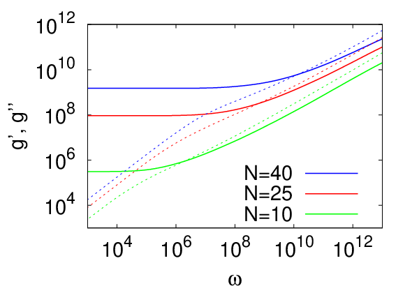
This gives , as expected from the dispersion () of the bending modes. The full numerical solution of Eq. (17) is presented in Fig. 2 for various crosslink densities . On small frequencies the static solution is recovered and leads to a plateau in the storage modulus, , where the value of the exponent depends on the type of quenched local network structure (angular brackets). The associated loss modulus scales linear with frequency and characterizes the viscous losses of a filament that moves with a velocity through the solvent.
IV Finite crosslink lifetime
If thermal fluctuations are comparable to the strength of a crosslink, then the bond will have a finite lifetime. In biological systems the crosslink-induced bonds between filaments usually have a lifetime in the range of seconds. The binding kinetics can therefore be picked up in standard rheological measurements. In fact, some systems display a pronounced peak in the loss modulus at the respective frequencies [29, 30].
In the following we explain how crosslink binding and unbinding can be introduced into the theory. Alternative theoretical developments are presented, for example, in Refs. [31, 32, 33]. We think of the crosslink to live in a one-dimensional periodic energy landscape that represents the binding states along the filament backbone (see Fig. 3). In f-actin the double-helical repeat implies a periodicity of roughly nm. While being bound at one site the crosslink stays in the respective minimum of the energy landscape, unbinding corresponds to Kramers escape from this minimum. In the fast-rebinding regime we can assume the crosslink to immediately fall in the neighboring minimum a distance away.
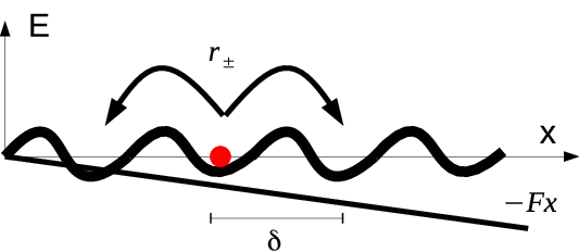
Via a force-dependent escape rate one direction is favored over the other. In linear response the crosslink then moves with a velocity and friction coefficient , as imposed by the fluctuation dissipation relation and a diffusion constant .
We thus conclude that crosslink binding/rebinding processes can be envisioned as a dash-pot that introduces viscous forces on the filaments, the friction coefficient being given in terms of microscopic properties of the crosslink and the binding domain of the filament.
With this insight the response function on the right side of Eqs. (13) and (14) have to be substituted (in frequency-space) by
| (20) |
representing a serial connection of crosslink binding domain and visco-elastic medium (Maxwell element).
This modifies Eq. (17) as follows
| (21) |
the diagonal matrix containing the Maxwell elements of the crosslink, .
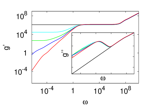
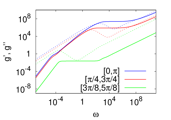
The result of this calculation can be seen in Figs. 4 and 5. Primarily, crosslink binding leads to the appearance of a Maxwell-like peak at small frequencies , where is the respective plateau modulus.
In Fig. 4 we display the rheology for a mixture of reversible and quenched (permanent) crosslinks. If there is a minimum number of quenched crosslinks per filament, there is a second plateau modulus at low frequencies. This indicates that these quenched crosslinks are sufficient in number to form a rigid structure – rigidity percolates.
In Fig. 5 we vary the structural randomness of the network. In particular, the distribution of crosslink angles is changed. As a result, a broad intermediate regime develops for the loss modulus, whenever the angles are broadly distributed. This regime reflects the spatial heterogeneity along the test filament. The ultimate low frequency regime () is only reached when all crosslinks along the test filament effectively behave equally.
V Nonlinear response
A full nonlinear theory has to include several factors, e.g. the reorientation of filaments under large strain [34] or the force-induced change in the polymer end-to-end distance. Also the effects of an applied prestress in combination with small amplitude oscillations is an important experimental probe. It is outside the scope of this work to fully combine all these aspects with our theoretical framework. However, progress is possible on a “schematic” level.
V.1 Prestress
To incorporate a constant prestress in our formalism, we make a “quasi-linear” approximation: We assume the linear theory to be valid, while we change the propagator
| (22) |
where the new -dependent term takes care of the reduction of transverse undulations by applying a tensile prestress. This results in a new stress-dependent plateau modulus , as well as a new regime at intermediate frequency (see Fig. 6). The frequency scale for this new scaling regime is , where is the wavelength of the relevant bending mode. In order for this regime to be accessible, the tension needs to be large enough to make , where is the relevant frequency scale without tension.

V.2 Schematic theory for strain ramp
Under large forces, the polymer will no longer behave as inextensible rod. Rather the specific form of the force-extension relation will become important. We can include this factor in a schematic model for the behavior under a strain ramp [35], where the strain linearly increases in time, .
This schematic model utilizes the key assumptions of Sects. II-IV: network strains translate into non-affine filament bending modes via a deformation of the tube; the amplitude of these bends grows linearly with strain (see Eq. (3)); the wavelengths of the bends are slaved to the surrounding network structure (factors ; see Fig. 1). The bending wavelengths are thus set by the typical inter-crosslink spacing. That is, if we consider a filament with crosslinks, the average bending wavelength will be .
Under larger strain, beyond the linear regime, two processes compete: first, non-linear filament elasticity (nonlinear force-extension relation) leads to strain-stiffening; second, cross- link unbinding leads to an increase in the wavelength of the bending modes and subsequently to strain-softening.
For a given bending amplitude , an associated longitudinal extension (increase of end-to-end distance) can be calculated via Pythagoras’ law, .
In response to large elastic deformations the crosslinks start to unbind (neglecting rebinding). Thus, the bending wavelength gets longer, as , and the elastic energy decreases. The interplay between stiffening and softening is then a competition between elastic stiffening (embodied in the non-linear longitudinal response) and softening via unbinding. To implement the softening part, we need a model for the elastic energy as well as a dynamical evolution equation for the crosslink number . The bending energy of the filament scales where we have used the bending spring constant of an elastic filament with bending stiffness . For the stretching energy we take the linearized force-extension relation of a wormlike chain with spring constant and the persistence length . The total energy then is , the force is the first derivative, the modulus is the second derivative with respect to strain. Without crosslink unbinding, this describes a strain- stiffening system. The strain-dependence in the non-linear regime follows from the longitudinal response and will be different, for example, when one considers an exponential stiffening model as in [32].
The simplest description for the crosslink dynamics is in terms of a rate equation
| (23) |
with forward rate and backward rate . Neglecting rebinding, . Unbinding happens at any one of crosslinks, thus , with an off-rate that may be force dependent, , with the -dependent force as given above. Solving the combined problem then gives Fig. 7. Similar curves have been found experimentally, for example in [35, 36, 37].


VI Conclusions
In conclusion, we have presented a theoretical framework for the linear and nonlinear visco-elastic properties of reversibly connected networks of semiflexible polymers. In our model the network strain does not couple directly to the filament end-to-end distance, but rather serves to locally distort the network structure. This induces bending modes in the filaments the amplitude of which grow linearly in strain, and the wavelength of wich are slaved to the local network structure, e.g. the distance to the next crosslink etc. Specifically, we investigated the frequency-dependent linear rheology, in particular in combination with crosslink binding/unbinding processes. Furthermore, we devised a schematic model for the nonlinear response in a creep experiment. These tests show that our model is capable of reproducing many of the key experimental findings available in the literature.
VII Acknowledgments
We acknowledge financial support by the German Science Foundation via the Emmy Noether program (He 6322/1-1) and via the collaborative research center SFB 937 (project A16).
References
- [1] A. Bausch and K. Kroy, Nature Physics 2, 231 (2006).
- [2] C. P. Broedersz and F. C. MacKintosh, Rev. Mod. Phys. 86, 995 (2014).
- [3] K. Kroy, Curr. Op. Coll. Int. Sc. 11, 56 (2006).
- [4] F. Gittes and F. C. MacKintosh, Phys. Rev. E 58, R1241 (1998).
- [5] E. Frey, K. Kroy, J. Wilhelm, and E. Sackmann, “Dynamical networks in physics and biology,” (Springer, Berlin, 1998) Chap. 9.
- [6] D. C. Morse, Phys. Rev. E 63, 031502 (2001).
- [7] J. L. Jones and R. C. Ball, Macromolecules 24, 6369 (1991).
- [8] L. Wolff, P. Fernandez, and K. Kroy, New Journal of Physics 12, 053024 (2010).
- [9] C. Heussinger and E. Frey, Phys. Rev. Lett. 97, 105501 (2006).
- [10] R. C. Picu, Soft Matter 7, 6768 (2011).
- [11] J. Wilhelm and E. Frey, Physical Review Letters 91(10) (2003).
- [12] D. A. Head, A. J. Levine, and F. C. MacKintosh, Physical Review Letters 91(10) (2003).
- [13] J. A. Åstrom, P. B. S. Kumar, and M. Karttunen, Soft Matter 5, 2869 (2009).
- [14] P. Müller and J. Kierfeld, Phys. Rev. Lett. 112, 094303 (2014).
- [15] M. Bai, A. R. Missel, W. S. Klug, and A. J. Levine, Soft Matter 7, 907 (2011).
- [16] F. C. MacKintosh, J. Käs, and P. A. Janmey, Phys. Rev. Lett. 75, 4425 (1995).
- [17] C. Storm, J. J. Pastore, F. C. MacKintosh, T. C. Lubensky, and P. A. Janmey, Nature 435, 191 (2005).
- [18] K. Kroy and J. Glaser, New J. Phys. 9, 416 (2007).
- [19] M. Das, D. A. Quint, and J. M. Schwarz, PLoS One 7, 35939 (2012).
- [20] X. Mao, O. Stenull, and T. C. Lubensky, Phys. Rev. E 87, 042601 (2013).
- [21] M. Sheinman, C. P. Broedersz, and F. C. MacKintosh, Phys. Rev. E 85, 021801 (2012).
- [22] C. P. Broedersz, X. Mao, T. C. Lubensky, and F. C. MacKintosh, Nat. Phys. 7, 983 (2011).
- [23] A. J. Liu, S. R. Nagel, W. van Saarloos, and M.Wyart, “The jamming scenario – an introduction and outlook,” (Oxford University Press, 2010) Chap. 9.
- [24] C. Heussinger, B. Schaefer, and E. Frey, Phys. Rev. E 76, 031906 (2007).
- [25] C. Heussinger and E. Frey, Eur. Phys. J. E 24, 47 (2007).
- [26] C. P. Broedersz, M. Sheinman, and F. C. MacKintosh, Phys. Rev. Lett. 108, 078102 (2012).
- [27] E. M. Huisman, C. Heussinger, C. Storm, and G. T. Barkema, Phys. Rev. Lett. 105, 118101 (2010).
- [28] In the following we will neglect the axial damping as well as the noise terms and . This does not qualitatively change the observed behavior.
- [29] O. Lieleg, M. M. A. E. Claessens, Y. Luan, and A. R. Bausch, Phys. Rev. Lett. 101, 108101 (2008).
- [30] C. P. Broedersz, M. Depken, N. Y. Yao, M. R. Pollak, D. A. Weitz, and F. C. MacKintosh, Phys. Rev. Lett. 105, 238101 (2010).
- [31] C. Vaca, R. Shlomovitz, Y. Yang, M. T. Valentine, and A. J. Levine, Soft Matter 11, 4899 (2015).
- [32] L. Wolff and K. Kroy, Phys. Rev. E 86, 040901 (2012).
- [33] C. Heussinger, New J. Phys. 14, 095029 (2012).
- [34] H. E. Amuasi, C. Heussinger, R. L. C. Vink, and A. Zippelius, New Journal of Physics 17, 083035 (2015).
- [35] M. Maier, K. Müller, C. Heussinger, S. Köhler, W. Wall, A. Bausch, and O. Lieleg, The European Physical Journal E 38, 50 (2015), 10.1140/epje/i2015-15050-3.
- [36] O. Lieleg, M. M. A. E. Claessens, and A. R. Bausch, Soft Matter 6, 218 (2010).
- [37] C. Semmrich, T. Storz, J. Glaser, R. Merkel, A. R. Bausch, and K. Kroy, Proceedings of the National Academy of Sciences 104, 20199 (2007), http://www.pnas.org/content/104/51/20199.full.pdf+html .