跳到论文正文
W Papers独立论文阅读器 arXiv:1602.03257 论文正文 计算阅读时间 · 0%
引用这篇论文根据当前论文元数据生成,正式投稿前建议核对。


License: arXiv.org perpetual non-exclusive license
arXiv:1602.03257v2 [math-ph] 01 May 2016

Asymptotics of mean-field O⁡(N)O(N) models

Kay Kirkpatrick Affiliation: Department of Mathematics, University of Illinois at Urbana-Champaign    Tayyab Nawaz ††thanks: Both authors partially supported by National Science Foundation (NSF) CAREER award DMS-1254791, and NSF grant 0932078 000 while in residence at Mathematical Sciences Research Institute (MSRI) during Fall 2015. Affiliation: 1409 W. Green Street, Urbana, IL 61801, USA
Abstract

We study mean-field classical NN-vector models, for integers N≥2N\geq 2. We use the theory of large deviations and Stein’s method to study the total spin and its typical behavior, specifically obtaining non-normal limit theorems at the critical temperatures and central limit theorems away from criticality. Important special cases of these models are the XY (N=2N=2) model of superconductors, the Heisenberg (N=3N=3) model (previously studied in [19] but with a correction to the critical distribution here), and the Toy (N=4N=4) model of the Higgs sector in particle physics.

keywords: Mean-field, Rate function, Total spin, Limit theorem, Phase transition.

1 Introduction

In statistical mechanics, mean-field models are often the starting point for understanding the behavior of the underlying physical systems, at least in high dimensions. In particular, we can use large deviations to study the asymptotics of physical quantities such as magnetization (total spin in our terminology) in models such as XY for superconductors, Heisenberg for ferromagnets [19], or the Toy model for particle physics. There is a family of models generalizing these important special cases, namely the mean-field classical NN-vector spin models, where each spin σi\sigma_{i} is in an NN-dimensional unit hypersphere, at a lattice site or in our case at a complete graph vertex ii among nn vertices. Then in the absence of an external field, each microstate or spin configuation σ=(σ1,σ2,…,σn)\sigma={(\sigma_{1},\sigma_{2},...,\sigma_{n})} in the configuration space Ωn=(𝕊N−1)n\Omega_{n}=(\mathbb{S}^{N-1})^{n} has a Hamiltonian defined by:

Hn(σ)=−∑i,jJi,j⟨σi,σj⟩.H_{n}(\sigma)=-\sum_{i,j}J_{i,j}\left\langle\sigma_{i},\sigma_{j}\right\rangle.

For the mean-field models defined on the complete graph, every two vertices (i,j)(i,j) are adjacent and the interaction between σi\sigma_{i} and σj\sigma_{j} is given by the constant Ji,j=12​nJ_{i,j}=\frac{1}{2n}, which can be viewed as an averaged interaction.

The N=1N=1 case of the mean-field NN-vector model is the Curie-Weiss model, which approximates the Ising model well for higher dimensions. The normalized total spin in the Curie-Weiss model has a non-Gaussian law in the non-critical regimes, and a law that converges to the distribution with density proportional to e−x4/12e^{-x^{4}/12} at the critical temperature (Ellis and Newman [14]). Chatterjee and Shao proved that the total spin at the critical temperature for this non-central limit theorem satisfies an error bound of order 1/n1/\sqrt{n} [6]. The XY model on a two-dimensional lattice is especially interesting for applications to superconductors [1], but challenging to study its phase transition rigorously.

For instance, the Mermin-Wagner theorem states that in two spatial dimensions, such a continuous symmetry cannot be broken spontaneously at any finite temperature [7]. This implies that the XY model on a two-dimensional lattice cannot have an ordered phase at low temperature like the Ising model does. Stanley and Moore provided some evidence that this system has a phase transition but it can’t be of usual type with finite mean magnetization below the critical temperature [17, 16]. But still in two dimensions it has an infinite-order transition names after Kosterlitz and Thouless (KT), who proved that there is phase transition from bound vortex-antivortex pairs at low temperature to unpaired vortices and anti-vortices at some critical temperature [15]. Above the transition temperature TK​TT_{KT} correlations between spins decay exponentially as usual, with some correlation length. They also showed that this system does not have any long-range order as the ground state is unstable against low-energy spin-wave excitations. They further proved that this is a low-temperature quasi-ordered phase with a correlation function that decreases with the distance like a power, which depends on the temperature.

Because the two-dimensional lattice XY model is challenging, the mean-field case is often the starting point for rigorous analysis of these spin models, a case that can be thought of as a large-dimensional limit of nearest-neighbor lattice models, or as an infinite limit for complete graph models. It is known that the classical NN-vector model with spins in 𝕊N−1\mathbb{S}^{N-1}, in the large-dimensional (d→∞d\to\infty) limit on the lattice ℤd\mathbb{Z}^{d}, has the critical inverse temperature βc=N\beta_{c}=N [21]. This limiting case is thought to approximate high-dimensional models well because magnetization goes to zero below the critical temperature for all dd, and the magnetization goes to the correct limit above the critical temperature as d→∞d\to\infty.

In this paper we study mean-field NN-vector models for positive integers NN, in the infinite limit for complete graphs. One reason for studying different dimensions collectively is because we can generate a family of solutions expressed in terms of modified Bessel functions, which can then be used for asymptotic analysis of the mean-field models. We have the following results:

  1. (a)

    Section 2 contains Large deviation principles (LDPs) for the total spin (with rate functions) and the empirical spin distribution (with relative entropies) for each non-negative inverse temperature.

  2. (b)

    Section 3 states the limit theorems for total spin in each phase, which are proved in sections 4 through 6.

  3. (c)

    Section 4 proves a central limit theorem in the subcritical (disordered) phase for the total spin, with Stein’s method.

  4. (d)

    Section 5 proves a CLT in the supercritical (ordered) phase for the total spin with a different scaling, again with Stein’s method.

  5. (e)

    Section 6 we derive a non-normal limit theorem for the total spin at the critical temperature, with limiting density of the squared length proportional to tN−22​e−14​N2​(N+2)​t2t^{\frac{N-2}{2}}e^{-\frac{1}{4N^{2}(N+2)}t^{2}}.

  6. (f)

    The Appendix contains some technical details including calculus for the free energy, and abstract results for the non-normal Stein’s method application.

2 The Setup and Large Deviations

We consider, for NN which is a fixed positive integer, the mean-field classical NN-vector, or O⁡(N)O(N), model on a complete graph KnK_{n} with nn vertices (these are isotropic models, meaning no external magnetic field). At each site ii on the graph is a spin σi\sigma_{i} in Ω=𝕊N−1\Omega=\mathbb{S}^{N-1}, so the state (or configuration) space is Ωn=(𝕊N−1)n\Omega_{n}=(\mathbb{S}^{N-1})^{n} with product measure PnP_{n} from the uniform probability measure on 𝕊N−1\mathbb{S}^{N-1}. For these models, and then the mean-field Hamiltonian energy Hn:Ωn→ℝH_{n}:\Omega_{n}\to\mathbb{R} is defined by:

Hn(σ):=−12​n∑i,j=1n⟨σi,σj⟩.H_{n}(\sigma):=-\frac{1}{2n}\sum_{i,j=1}^{n}\left\langle\sigma_{i},\sigma_{j}\right\rangle.

The energy per particle is hn​(σ)=1n​Hn​(σ)h_{n}(\sigma)=\frac{1}{n}H_{n}(\sigma), and the canonical ensemble, or Gibbs measure, is the probability measure Pn,βP_{n,\beta} on Ωn\Omega_{n} with density (with respect to PnP_{n}):

f⁡(σ):=1Z​e−β​Hn​(σ)=1Z​exp⁡(β2​n​∑i,j=1n⟨σi,σj⟩).f(\sigma):=\frac{1}{Z}e^{-\beta H_{n}(\sigma)}=\frac{1}{Z}\exp\left(\frac{\beta}{2n}\sum_{i,j=1}^{n}\left\langle\sigma_{i},\sigma_{j}\right\rangle\right).

The (normalizing) partition function is given by:

Z=Zn​(β)=∫Ωnexp⁡(β2​n​∑i,j=1n⟨σi,σj⟩)​d​Pn.Z=Z_{n}(\beta)=\int_{\Omega_{n}}\exp\left(\frac{\beta}{2n}\sum_{i,j=1}^{n}\left\langle\sigma_{i},\sigma_{j}\right\rangle\right)dP_{n}.

We will call M1​(𝕊N−1)M_{1}(\mathbb{S}^{N-1}) the space of probability measures on 𝕊N−1\mathbb{S}^{N-1} with the weak-* topology.

Now we are interested in studying the behavior of the important physical quantity of total spin Sn:=∑i=1nσiS_{n}:=\sum_{i=1}^{n}\sigma_{i} in terms of the inverse temperature β\beta, distributed according to the Gibbs measures. First we present a proposition stating the large deviation principle for the empirical spin distribution for non-interacting particles (disordered infinite-temperature case) β=0\beta=0, a proposition that is a special case of Sanov’s theorem.

Proposition 1.

If PnP_{n} is the nn-fold product of uniform measure on 𝕊N−1\mathbb{S}^{N-1}, μn,σ=1n​∑i=1nδσi\mu_{n,\sigma}=\frac{1}{n}\sum_{i=1}^{n}\delta_{\sigma_{i}} is the empirical spin distribution, and Γ\Gamma a Borel subset of M1​(𝕊N−1)M_{1}(\mathbb{S}^{N-1}), then

−infν∈Γ∘H(ν∣μ)\displaystyle-\inf_{\nu\in\Gamma^{\circ}}H(\nu\mid\mu) ≤lim infn→∞1nlogPn[μn,σ∈Γ]\displaystyle\leq\liminf_{n\to\infty}\frac{1}{n}\log P_{n}[\mu_{n,\sigma}\in\Gamma]
≤lim supn→∞1nlogPn[μn,σ∈Γ]≤−infν∈Γ¯H(ν∣μ);\displaystyle\leq\limsup_{n\to\infty}\frac{1}{n}\log P_{n}[\mu_{n,\sigma}\in\Gamma]\leq-\inf_{\nu\in\overline{\Gamma}}H(\nu\mid\mu);

i.e., the random measures μn,σ\mu_{n,\sigma} satisfy an LDP with rate function H(⋅∣μ)H(\cdot\mid\mu), the relative entropy, defined for a probability measure ν\nu on 𝕊N−1\mathbb{S}^{N-1}, with respect to uniform measure μ\mu, by:

H(ν∣μ):={∫𝕊N−1f​log⁡(f)​𝑑μif​f:=d​νd​μ​exists;∞otherwise.H(\nu\mid\mu):=\begin{cases}\int_{\mathbb{S}^{N-1}}f\log(f)d\mu&\text{if}\,\,f:=\frac{d\nu}{d\mu}\,\,\text{exists};\\ \infty&\text{otherwise}.\end{cases}

In particular, at infinite temperature β=0\beta=0, the unique minimizer of the rate function is the uniform measure μ\mu, meaning that spins are uniformly and independently distributed on the sphere, with no preferred direction in this disordered phase.

Now we state the general case β≥0\beta\geq 0, which follows from abstract results of Ellis, Haven, and Turkington ([13], Theorems 2.4 and 2.5):

Theorem 2.

If β≥0\beta\geq 0 then the empirical spin distributions μn,σ\mu_{n,\sigma} satisfy an LDP on M1​(𝕊N−1)M_{1}(\mathbb{S}^{N-1}) with rate function:

Iβ​(ν):=H⁡(ν∣μ)−β2​|∫𝕊N−1x​𝑑ν​(x)|2−φ⁡(β),I_{\beta}(\nu):=H(\nu\mid\mu)-\frac{\beta}{2}\left|\int_{\mathbb{S}^{N-1}}xd\nu(x)\right|^{2}-\varphi(\beta), (1)

where φ\varphi is the free energy defined by φ(β):=−limn→∞1nlogZn(β)\varphi(\beta):=-\lim_{n\to\infty}\frac{1}{n}\log Z_{n}(\beta), which exists and is given by the alternative formula:

φ⁡(β)=infν∈M1​(𝕊N−1)[H⁡(ν∣μ)−β2​|∫𝕊N−1x​𝑑ν​(x)|2].\varphi(\beta)=\inf_{\nu\in M_{1}(\mathbb{S}^{N-1})}\left[H(\nu\mid\mu)-\frac{\beta}{2}\left|\int_{\mathbb{S}^{N-1}}xd\nu(x)\right|^{2}\right]. (2)

Remarks on notation:

  1. (a)

    Throughout this paper we will write the rate function as IβI_{\beta} where the subscript is the real, non-negative inverse temperature β=1/(kB​T)\beta=1/(k_{B}T), where TT is temperature and kBk_{B} is the Boltzmann constant; we will write the modified Bessel function of the first kind as InI_{n} where nn is an integer.

  2. (b)

    The average magnetization m=𝔼⁡[1n​Sn]=𝔼⁡[1n​∑iσi]m=\mathbb{E}[\frac{1}{n}S_{n}]=\mathbb{E}[\frac{1}{n}\sum_{i}\sigma_{i}] for the NN-vector spin model can be calculated by differentiating the partition function and comes out to be, in terms of Bessel functions:

    |m|=IN2​(|x|)IN2−1​(|x|).|m|=\frac{I_{\frac{N}{2}}(|x|)}{I_{\frac{N}{2}-1}(|x|)}.
  3. (c)

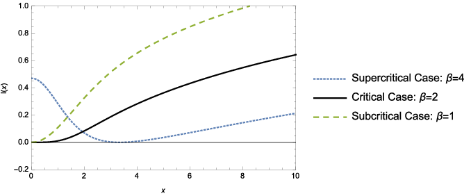
    We can also verify that the rate functions IβI_{\beta} are always nonnegative, as illustrated in Figure 1 below for N=2N=2 in three representative cases of β\beta.

    Refer to caption
    Figure 1: Rate Function IβI_{\beta} for the mean-field XY Model
Theorem 3.

For dimension NN , the free energy φ\varphi has the formula:

φ⁡(β)={0, if ​β<N,Φβ​(Υ−1​(β)), if ​β≥N,\varphi(\beta)=\begin{cases}0,\quad\quad\quad\quad\quad\quad\quad\quad\text{ if }\beta<N,\\ \Phi_{\beta}(\Upsilon^{-1}(\beta)),\quad\quad\quad\;\,\text{ if }\beta\geq N,\end{cases}

where for r=Υ−1​(β)r=\Upsilon^{-1}(\beta),

Φβ​(r)=r​IN2​(r)IN2−1​(r)+log⁡[ANAN−1​rN2−1BN​π​IN2−1​(r)]−β2​(IN2​(r)IN2−1​(r))2,\Phi_{\beta}(r)=r\frac{I_{\frac{N}{2}}(r)}{I_{\frac{N}{2}-1}(r)}+\log\left[\frac{A_{N}}{A_{N-1}}\frac{r^{\frac{N}{2}-1}}{B_{N}\pi I_{\frac{N}{2}-1}(r)}\right]-\frac{\beta}{2}\left(\frac{I_{\frac{N}{2}}(r)}{I_{\frac{N}{2}-1}(r)}\right)^{2},

with

AN:=2​πN2Γ⁡(N2),Υ⁡(r)=ΥN​(r):=r​IN2−1​(r)IN2​(r)=β,A_{N}:=\frac{2\pi^{\frac{N}{2}}}{\Gamma{\left(\frac{N}{2}\right)}},\quad\quad\Upsilon(r)=\Upsilon_{N}(r):=r\frac{I_{\frac{N}{2}-1}(r)}{I_{\frac{N}{2}}(r)}=\beta,

and

BN={∏k=0N2−1|2​k−1|, if N even,2N−32​(1)N−32, if N odd,B_{N}=\begin{cases}\prod_{k=0}^{\frac{N}{2}-1}|2k-1|,\quad\quad\quad\quad\quad\quad\quad\quad\text{ if N even},\\ \\ 2^{\frac{N-3}{2}}(1)_{\frac{N-3}{2}},\quad\quad\quad\quad\quad\quad\quad\quad\quad\;\,\text{ if N odd},\end{cases}

where (a)n(a)_{n} is pochhammer symbol. In particular, we find the critical threshold β=N\beta=N, and we can check by calculating limits that φ\varphi and φ′\varphi^{\prime} are continuous, implying that the phase transition is continuous.

We can precisely describe the phase transition in free energy as follows:

  • •

    For 0≤β≤βc=N0\leq\beta\leq\beta_{c}=N, we obtain unique global minima for free energy at the origin with a zero magnetization.

  • •

    For β≥βc=N\beta\geq\beta_{c}=N, we have infinitely many global minima for the free energy which can be approximated graphically. Furthermore, the minima in this case are identical with non-zero magnetization.

We can deduce from Proposition 1 the following Cramér-type LDP for the average spin Mn:=1n​Sn=1n​∑i=1nσiM_{n}:=\frac{1}{n}S_{n}=\frac{1}{n}\sum_{i=1}^{n}\sigma_{i} in the noninteracting case β=0\beta=0 (or alternatively prove this Cramér theorem directly for random vectors on the hypersphere).

Corollary 4.

If {σi}i=1n\{\sigma_{i}\}_{i=1}^{n} are i.i.d. uniform random points on 𝕊N−1⊆ℝN\mathbb{S}^{N-1}\subseteq\mathbb{R}^{N}, then for r=|x|r=|x|, the average spins MnM_{n} satisfy an LDP with rate function II:

Pn​(Mn≃x)≃e−n​I​(r),P_{n}\left(M_{n}\simeq x\right)\simeq e^{-nI(r)},

where I​(r)=Φ0​(r)I(r)=\Phi_{0}(r) from Theorem 3.

Similarly we have a Cramér-type result for the interacting case β>0\beta>0 as follows:

Proposition 5.

If Mn=Mn​(σ):=1n​∑i=1nσiM_{n}=M_{n}(\sigma):=\frac{1}{n}\sum_{i=1}^{n}\sigma_{i} and Pn,βP_{n,\beta} is the Gibbs measure as defined above, then for a Borel set Γ∈ℝ\Gamma\in\mathbb{R},

−infx∈Γ∘Iβ(x)\displaystyle-\inf_{x\in\Gamma^{\circ}}I_{\beta}(x) ≤lim infn→∞1nlogPn,β[βMn∈Γ]\displaystyle\leq\liminf_{n\to\infty}\frac{1}{n}\log P_{n,\beta}\left[\beta M_{n}\in\Gamma\right]
≤lim supn→∞1nlogPn,β[βMn∈Γ]≤−infx∈Γ¯Iβ(x)\displaystyle\leq\limsup_{n\to\infty}\frac{1}{n}\log P_{n,\beta}\left[\beta M_{n}\in\Gamma\right]\leq-\inf_{x\in\overline{\Gamma}}I_{\beta}(x)

where for r=|x|r=|x|,

Iβ​(r)=Φβ​(r)−infν∈M1​(𝕊N−1)Φβ​(r),I_{\beta}(r)=\Phi_{\beta}(r)-\inf_{\nu\in M_{1}(\mathbb{S}^{N-1})}\Phi_{\beta}(r),

and Φβ​(r)\Phi_{\beta}(r) is defined in Theorem 3.

Using similar reasoning as [19], we consider the measure νg\nu_{g} with the density function

f⁡(x1,x2,…,xN)=g⁡(xN)f(x_{1},x_{2},...,x_{N})=g(x_{N})

which is increasing in xNx_{N}. This gives:

H⁡(νg∣μ)=∫𝕊N−1f⁡(x1,x2,…,xN)​log⁡[f⁡(x1,x2,…,xN)]​d​x1​d​x2​…​d​xN=1AN​∫0π∫0π…​∫0π∫02​πg⁡(cos⁡(θN−1))​log⁡[g⁡(cos⁡(θN−1))]∏k=2N−1S​i​nk−1​(θk)​d​θ1​d​θ2​…​d​θN−1=AN−1AN​∫0πg⁡(cos⁡(θN−1))​log⁡[g⁡(cos⁡(θN−1))]​S​i​nN−2​(θN−1)​d​θN−1=AN−1AN​∫−11g⁡(xN)​log⁡[g⁡(xN)]​(1−xN2)N−32​d​xN.\begin{split}H(\nu_{g}\mid\mu)&=\int_{\mathbb{S}_{N-1}}f(x_{1},x_{2},...,x_{N})\log[f(x_{1},x_{2},...,x_{N})]dx_{1}dx_{2}...dx_{N}\\ &=\frac{1}{A_{N}}\int_{0}^{\pi}\int_{0}^{\pi}...\int_{0}^{\pi}\int_{0}^{2\pi}g(\cos(\theta_{N-1}))\log[g(\cos(\theta_{N-1}))]\\ &~~~~~~~~~~~~~~~~~~~~~~~~~~~~~~~~~~\prod_{k=2}^{N-1}Sin^{k-1}(\theta_{k})d\theta_{1}d\theta_{2}...d\theta_{N-1}\\ &=\frac{A_{N-1}}{A_{N}}\int_{0}^{\pi}g(\cos(\theta_{N-1}))\log[g(\cos(\theta_{N-1}))]Sin^{N-2}(\theta_{N-1})d\theta_{N-1}\\ &=\frac{A_{N-1}}{A_{N}}\int_{-1}^{1}g(x_{N})\log[g(x_{N})]\left(1-x_{N}^{2}\right)^{\frac{N-3}{2}}dx_{N}.\end{split}

Similarly, if eNe_{N} is the unit coordinate vector in direction xNx_{N}, then

∫𝕊N−1v​d​νg​(v)=eN​AN−1AN​∫−11xN​g​(xN)​(1−xN2)N−32​d​xN.\int_{\mathbb{S}^{N-1}}vd\nu_{g}(v)=e_{N}\frac{A_{N-1}}{A_{N}}\int_{-1}^{1}x_{N}g(x_{N})\left(1-x_{N}^{2}\right)^{\frac{N-3}{2}}dx_{N}.

Now we are interested in minimizing the functional

AN−1AN​∫−11g⁡(xN)​log⁡[g⁡(xN)]​(1−xN2)N−32​d​xN−β2​(AN−1AN​∫−11xN​g​(xN)​(1−xN2)N−32​d​xN)2\frac{A_{N-1}}{A_{N}}\int_{-1}^{1}g(x_{N})\log[g(x_{N})]\left(1-x_{N}^{2}\right)^{\frac{N-3}{2}}dx_{N}-\frac{\beta}{2}\left(\frac{A_{N-1}}{A_{N}}\int_{-1}^{1}x_{N}g(x_{N})\left(1-x_{N}^{2}\right)^{\frac{N-3}{2}}dx_{N}\right)^{2}

under the following constraint: g:[−1,1]→ℝ+g:[-1,1]\to\mathbb{R}_{+} increasing and such that

AN−1AN​∫−11g⁡(xN)​(1−xN2)N−32​d​xN=1.\frac{A_{N-1}}{A_{N}}\int_{-1}^{1}g(x_{N})\left(1-x_{N}^{2}\right)^{\frac{N-3}{2}}dx_{N}=1.

We can also write the functional under consideration in terms of entropy as follows:

AN−1AN​∫−11g⁡(xN)​log⁡[g⁡(xN)]​(1−xN2)N−32​d​xN=AN−1AN​∫−11g⁡(xN)​log⁡[g⁡(xN)​ANAN−1]​(1−xN2)N−32​d​xN+log⁡[AN−1AN]=−ξ⁡(g​ANAN−1)+log⁡[AN−1AN],\begin{split}&\frac{A_{N-1}}{A_{N}}\int_{-1}^{1}g(x_{N})\log[g(x_{N})]\left(1-x_{N}^{2}\right)^{\frac{N-3}{2}}dx_{N}\\ &=\frac{A_{N-1}}{A_{N}}\int_{-1}^{1}g(x_{N})\log\left[\frac{g(x_{N})A_{N}}{A_{N-1}}\right]\left(1-x_{N}^{2}\right)^{\frac{N-3}{2}}dx_{N}+\log\left[\frac{A_{N-1}}{A_{N}}\right]\\ &=-\xi\left(\frac{gA_{N}}{A_{N-1}}\right)+\log\left[\frac{A_{N-1}}{A_{N}}\right],\end{split}

where ξ⁡(ϕ)\xi\left(\phi\right) is the entropy of the density ϕ\phi.

Now using constrained entropy optimization (Theorem 12.1.1 in [9]), we fix c∈[0,1]c\in[0,1] and minimize the above quantity over the measures ν∈M1​(𝕊N−1)\nu\in M_{1}(\mathbb{S}^{N-1}) such that |∫𝕊N−1x​𝑑ν​(x)|=c.\left|\int_{\mathbb{S}^{N-1}}xd\nu(x)\right|=c.

Proposition 6.

Consider the set of functions h:[−1,1]→ℝ+h:[-1,1]\to\mathbb{R}_{+} such that

  1. (a)

    ∫−11h⁡(xN)​(1−xN2)N−32​d​xN=1\int_{-1}^{1}h(x_{N})\left(1-x_{N}^{2}\right)^{\frac{N-3}{2}}dx_{N}=1, and

  2. (b)

    |∫−11xN​h​(xN)​(1−xN2)N−32​d​xN|=c\left|\int_{-1}^{1}x_{N}h(x_{N})\left(1-x_{N}^{2}\right)^{\frac{N-3}{2}}dx_{N}\right|=c.

Then in the set of functions satisfying these conditions, h∗​(x)=a​eb​xh^{*}(x)=ae^{bx} uniquely minimizes the quantity

AN−1AN​∫−11g⁡(xN)​log⁡[g⁡(xN)]​(1−xN2)N−32​d​xN.\frac{A_{N-1}}{A_{N}}\int_{-1}^{1}g(x_{N})\log[g(x_{N})]\left(1-x_{N}^{2}\right)^{\frac{N-3}{2}}dx_{N}.

Now we will use the conditions (a)(a) and (b)(b) to find the values of the parameters aa and bb for the function h∗h^{*}. The first condition leads us to the following two subcases: for NN even,

1=∫−11a​eb​xN​(1−xN2)N−32​d​xN=(∏k=0N2−1|2​k−1|)​a​π​IN2−1​(b)bN2−1,1=\int_{-1}^{1}ae^{bx_{N}}\left(1-x_{N}^{2}\right)^{\frac{N-3}{2}}dx_{N}=\frac{\left(\prod_{k=0}^{\frac{N}{2}-1}|2k-1|\right)a\pi I_{\frac{N}{2}-1}(b)}{b^{\frac{N}{2}-1}},

which implies

a=bN2−1(∏k=0N2−1|2​k−1|)​π​IN2−1​(b)a=\frac{b^{\frac{N}{2}-1}}{\left(\prod_{k=0}^{\frac{N}{2}-1}|2k-1|\right)\pi I_{\frac{N}{2}-1}(b)}

Now using second condition, For NN even, we have

c=∫−11xN​h​(xN)​(1−xN2)N−32​d​xN=(∏k=0N2−1|2​k−1|)​a​π​IN2​(b)bN2−1=IN2​(b)IN2−1​(b).\begin{split}c&=\int_{-1}^{1}x_{N}h(x_{N})\left(1-x_{N}^{2}\right)^{\frac{N-3}{2}}dx_{N}=\frac{\left(\prod_{k=0}^{\frac{N}{2}-1}|2k-1|\right)a\pi I_{\frac{N}{2}}(b)}{b^{\frac{N}{2}-1}}=\frac{I_{\frac{N}{2}}(b)}{I_{\frac{N}{2}-1}(b)}.\end{split}

Let g∗=(AN−1AN)​h∗g^{*}=\left(\frac{A_{N-1}}{A_{N}}\right)h^{*}; and c∈[0,1]c\in[0,1] with g∗g^{*} increasing corresponds to considering all b∈[0,∞)b\in[0,\infty). Now we have to minimize for NN even,

AN−1AN​∫−11g⁡(xN)​log⁡[g⁡(xN)]​(1−xN2)N−32​d​xN−β2​(AN−1AN​∫−11xN​g​(xN)​(1−xN2)N−32​d​xN)2=b​IN2​(b)IN2−1​(b)+log⁡[ANAN−1​bN2−1(∏k=0N2−1|2​k−1|)​π​IN2−1​(b)]−β2​(IN2​(b)IN2−1​(b))2=:Φβ​(b)\begin{split}&\frac{A_{N-1}}{A_{N}}\int_{-1}^{1}g(x_{N})\log[g(x_{N})]\left(1-x_{N}^{2}\right)^{\frac{N-3}{2}}dx_{N}-\frac{\beta}{2}\left(\frac{A_{N-1}}{A_{N}}\int_{-1}^{1}x_{N}g(x_{N})\left(1-x_{N}^{2}\right)^{\frac{N-3}{2}}dx_{N}\right)^{2}\\ &=b\frac{I_{\frac{N}{2}}(b)}{I_{\frac{N}{2}-1}(b)}+\log\left[\frac{A_{N}}{A_{N-1}}\frac{b^{\frac{N}{2}-1}}{\left(\prod_{k=0}^{\frac{N}{2}-1}|2k-1|\right)\pi I_{\frac{N}{2}-1}(b)}\right]-\frac{\beta}{2}\left(\frac{I_{\frac{N}{2}}(b)}{I_{\frac{N}{2}-1}(b)}\right)^{2}\\ &=:\Phi_{\beta}(b)\end{split} (3)

over all b∈[0,∞)b\in[0,\infty). Using same approach we can derive the expression for Φβ​(b)\Phi_{\beta}(b), for NN odd and this comes out to be

Φβ​(b)=b​IN2​(b)IN2−1​(b)+log⁡[ANAN−1​bN2−1(2N−32​(1)N−32)​π​IN2−1​(b)]−β2​(IN2​(b)IN2−1​(b))2,\Phi_{\beta}(b)=b\frac{I_{\frac{N}{2}}(b)}{I_{\frac{N}{2}-1}(b)}+\log\left[\frac{A_{N}}{A_{N-1}}\frac{b^{\frac{N}{2}-1}}{\left(2^{\frac{N-3}{2}}(1)_{\frac{N-3}{2}}\right)\pi I_{\frac{N}{2}-1}(b)}\right]-\frac{\beta}{2}\left(\frac{I_{\frac{N}{2}}(b)}{I_{\frac{N}{2}-1}(b)}\right)^{2},

where (a)n(a)_{n} represents pochhammer symbol. This is now one-dimensional problem which is studied in Lemma 16 in Appendix. We deduce that βc=N\beta_{c}=N is the critical inverse temperature. Also for β<N\beta<N we have the uniform distribution as the only macrocanonical state whereas for β>N\beta>N we have a family (parametrized by the circle) of distributions with a preferred direction (and converging to a family of points masses, each concentrated on a perfectly preferred direction as β→∞\beta\to\infty). We can state the following theorem using our calculations from Lemma 16:

Theorem 7.
  1. (a)

    For β≤N\beta\leq N, the expression (3) is minimized for b=0b=0, then the corresponding a=1a=1, so that the minimizing function h∗=1h^{*}=1 and hence the canonical macrostates in the subcritical case are uniform: ℰβ={μ}\mathcal{E}_{\beta}=\{\mu\}.

  2. (b)

    In the supercritical case, β>N\beta>N, the minimizing bb for the expression (3) is the unique strictly positive solution to

    b=β⁡(IN2​(b)IN2−1​(b)),b=\beta\left(\frac{I_{\frac{N}{2}}(b)}{I_{\frac{N}{2}-1}(b)}\right),

    which moreover has limit limβ↓βcb=0\lim_{\beta\downarrow\beta_{c}}b=0.The macrostates ℰβ\mathcal{E}_{\beta} are given by {νx}x∈𝕊N−1,\{\nu_{x}\}_{x\in\mathbb{S}^{N-1}}, where νx\nu_{x} is the probability measure with density which is symmetric about the pole at xx, with density gx:[−1,1]→ℝg_{x}:[-1,1]\to\mathbb{R} in the xx-direction given by (AN−1AN)​a​eb​x\left(\frac{A_{N-1}}{A_{N}}\right)ae^{bx} with bb as above.

3 Limit Theorems for the Total Spin

We study the total spin in the subcritical, critical, and supercritical regimes, proving central and non-central limit theorems for the total spin, holding NN, the dimension of the spin, fixed. In this section we state these limit theorems for each regime and give the proofs of each one of these in next few sections.

In the subcritical regime 0≤β<N0\leq\beta<N, the spins are weakly correlated and hence can be treated similar to the independent case β=0\beta=0. The average magnetization of the system is very small and goes to zero with increasing number of spins n→∞n\to\infty for this high temperature regime. In this regime we have the following multivariate central limit theorem, and in particular, the macrostate is the uniform measure on the hypersphere.

Theorem 8.

In the subcritical regime β<N\beta<N, the random variable WnW_{n} is defined as follows: Wn=N−βn​∑i=1nσiW_{n}=\sqrt{\frac{N-\beta}{n}}\sum_{i=1}^{n}\sigma_{i} Then

supg:L⁡(g),M⁡(g)≤1|𝔼g(Wn)−𝔼g(Z)|≤cβn\sup_{g:L(g),M(g)\leq 1}|\mathbb{E}g(W_{n})-\mathbb{E}g(Z)|\leq\frac{c_{\beta}}{\sqrt{n}}

where cβc_{\beta} is a constant depending only on β\beta, L⁡(g)L(g) is the Lipschitz constant of gg, M⁡(g)M(g) is the maximum operator norm of the Hessian of gg, and ZZ is a standard Gaussian random vector in ℝN\mathbb{R}^{N}.

Remark: Our rate of convergence for Theorem 8 is sharper than [19], which had a factor of log⁡(n)\log(n) in the numerator, based on an argument of Leslie Ross [22]. The supremum in Theorem 8 is a metric for the topology of weak-* convergence and convergence in mean on the space M1​(𝕊N−1)M_{1}(\mathbb{S}^{N-1}) of probability measures on the hypersphere.

In the supercritical regime β>N\beta>N, the spins align to some extent: For smaller values of β>N\beta>N, the spins show a slight preference for a particular (random) direction, whereas for large β\beta, the spins align strongly. Consider a small interval Γ\Gamma containing bb, now using the fact that infx∈Γ¯Iβ​(x)=b\inf_{x\in\overline{\Gamma}}I_{\beta}(x)=b and Proposition 5, we conclude that |Sn||S_{n}| has a high probability of being close to b​n/βbn/\beta. Here all points on the hypersphere of radius b​n/βbn/\beta will have equal probability due to symmetry. Using an argument similar to [19], we consider the fluctuations of squared-length of total spin, i.e., we consider the following random variable:

Wn:=n​[β2n2​b2​|∑j=1nσj|2−1].W_{n}:=\sqrt{n}\left[\frac{\beta^{2}}{n^{2}b^{2}}\left|\sum_{j=1}^{n}\sigma_{j}\right|^{2}-1\right]. (4)

In Section 5, we prove that this WnW_{n} satisfies the following central limit theorem.

Theorem 9.

If WnW_{n} is as defined in (4) and bb is the solution of b−β​f​(b)=0,b-\beta f(b)=0, where

f⁡(b)=IN2​(b)IN2−1​(b),f(b)=\frac{I_{\frac{N}{2}}(b)}{I_{\frac{N}{2}-1}(b)},

then there is a constant cβc_{\beta} depending on β>N\beta>N only, such that if ZZ is a centered normal random variable with variance

V​a​r​(σ)=4​β2(1−β​f′​(b))​b2​[1−N−1N​(IN2−1​(b)+IN2+1​(b))IN2−1​(b)−(IN2​(b)IN2−1​(b))2]Var(\sigma)=\frac{4\beta^{2}}{\left(1-\beta f^{\prime}(b)\right)b^{2}}\left[1-\frac{N-1}{N}\frac{\left(I_{\frac{N}{2}-1}(b)+I_{\frac{N}{2}+1}(b)\right)}{I_{\frac{N}{2}-1}(b)}-\left(\frac{I_{\frac{N}{2}}(b)}{I_{\frac{N}{2}-1}(b)}\right)^{2}\right]

then

dB​L​(Wn,Z)≤cβ​(log⁡(n)n)1/4.d_{BL}(W_{n},Z)\leq c_{\beta}\left(\frac{\log(n)}{n}\right)^{1/4}.

Here the bounded Lipschitz distance dB​L​(X,Y)d_{BL}(X,Y) between random variables XX and YY is:

dB​L(X,Y):=sup{|𝔼h(X)−𝔼h(Y)|:∥h∥∞≤1,M1(h)≤1},d_{BL}(X,Y):=\sup\left\{\Big|\mathbb{E}h(X)-\mathbb{E}h(Y)\Big|:\|h\|_{\infty}\leq 1,M_{1}(h)\leq 1\right\}, (5)

where ∥⋅∥∞\|\cdot\|_{\infty} is the supremum norm and L⁡(⋅)L(\cdot) is the Lipschitz constant as before.

We can obtain the complete asymptotic behavior of the total spin without using conditioning (as in e.g., [14]) by using instead the rotational invariance of the total spin, a strategy adapted from [19].

In Section 6, we prove the following nonnormal limit theorem for the random variable defined by

Wn:=cN​|Sn|2n32.W_{n}:=\frac{c_{N}|S_{n}|^{2}}{n^{\frac{3}{2}}}. (6)

at the critical temperature β=N\beta=N. Because of symmetry of the total spin this leads us to the limiting picture in the critical case. The critical limiting density function pp (defined below) is obtained using Stein’s method similar to [6, 19].

Theorem 10.

If we consider the critical temperature β=N\beta=N, and WnW_{n} as defined by (6) , and if XX is the random variable with the density

p⁡(t)={1z​tN−22​e−14​N2​(N+2)​t2t≥0;0t<0,,p(t)=\begin{cases}\frac{1}{z}t^{\frac{N-2}{2}}e^{-\frac{1}{4N^{2}(N+2)}t^{2}}&t\geq 0;\\ 0&t<0,\end{cases},

where zz is normalizing constant and cNc_{N} is such that 𝔼​Wn=1\mathbb{E}W_{n}=1, then there exists a universal constant CC such that

sup‖h‖∞≤1,‖h′‖∞≤1‖h′′‖∞≤1|𝔼​h​(Wn)−𝔼​h​(X)|≤C​log⁡(n)n.\sup_{\begin{subarray}{c}\|h\|_{\infty}\leq 1,\,\|h^{\prime}\|_{\infty}\leq 1\\ \|h^{\prime\prime}\|_{\infty}\leq 1\end{subarray}}\big|\mathbb{E}h(W_{n})-\mathbb{E}h(X)\big|\leq\frac{C\log(n)}{\sqrt{n}}.

4 The Subcritical Phase

This section has the proof of Theorem 8, the limit theorem for SnS_{n} in the disordered phase. We start by calculating the variance of the total spin Sn:=∑i=1nσiS_{n}:=\sum_{i=1}^{n}\sigma_{i}. Since the density of the Gibbs measure is symmetric and in particular rotationally invariant, each of the spins σi\sigma_{i} has a uniform marginal distribution, and 𝔼⁡⟨σi,σi⟩=1\mathbb{E}\left\langle\sigma_{i},\sigma_{i}\right\rangle=1 for each ii and 𝔼⁡⟨σi,σj⟩\mathbb{E}\left\langle\sigma_{i},\sigma_{j}\right\rangle is the same for every pair i≠ji\neq j.

Following [19], the density of σ1\sigma_{1} with respect to uniform measure on 𝕊N−1\mathbb{S}^{N-1}, conditional on {σj}j≠1\{\sigma_{j}\}_{j\neq 1}, is

Z1−1​exp⁡[βn​∑j≠1⟨θ,σj⟩],Z_{1}^{-1}\exp\left[\frac{\beta}{n}\sum_{j\neq 1}\left\langle\theta,\sigma_{j}\right\rangle\right],

where Z1=∫𝕊N−1exp⁡[βn​∑j≠1⟨θ,σj⟩]​𝑑μ​(θ)Z_{1}=\int_{\mathbb{S}^{N-1}}\exp\left[\frac{\beta}{n}\sum_{j\neq 1}\left\langle\theta,\sigma_{j}\right\rangle\right]d\mu(\theta) is the normalization factor. If i∈{1,…,n}i\in\{1,\ldots,n\} is fixed, then call σ(i):=∑j≠iσj\sigma^{(i)}:=\sum_{j\neq i}\sigma_{j}. We use hyperspherical coordinates,

d​μ​(θ)=JNAN​d​θ1​…​d​θN−1,d\mu(\theta)=\frac{J_{N}}{A_{N}}d\theta_{1}\dots d\theta_{N-1},

where

JN=(−1)N−1​∏k=2N−1sink−1⁡(θk).J_{N}=\left(-1\right)^{N-1}\prod_{k=2}^{N-1}\sin^{k-1}(\theta_{k}).

Here AN=2​πN2/Γ⁡(N2)A_{N}=2\pi^{\frac{N}{2}}/\Gamma{\left(\frac{N}{2}\right)}, and we also use the notation κ=β​|σ(1)|n\kappa=\frac{\beta|\sigma^{(1)}|}{n}. Therefore the normalization factor is

Z1\displaystyle Z_{1} =1AN​∫0π…​∫0π∫02​πeκ​cos⁡(θN−1)​JN​d​θ1​…​d​θN−2​d​θN−1\displaystyle=\frac{1}{A_{N}}\int_{0}^{\pi}...\int_{0}^{\pi}\int_{0}^{2\pi}e^{\kappa\cos(\theta_{N-1})}J_{N}d\theta_{1}...d\theta_{N-2}d\theta_{N-1}
=1AN​∫0π…​∫0π∫02​πeκ​cos⁡(θN−1)​sin⁡(θ2)​sin2⁡(θ3)​…​sinN−2⁡(θN−1)​d​θ1​…​d​θN−2​d​θN−1\displaystyle=\frac{1}{A_{N}}\int_{0}^{\pi}...\int_{0}^{\pi}\int_{0}^{2\pi}e^{\kappa\cos(\theta_{N-1})}\sin(\theta_{2})\sin^{2}(\theta_{3})...\sin^{N-2}(\theta_{N-1})d\theta_{1}...d\theta_{N-2}d\theta_{N-1}
=AN−1AN​∫0πeκ​cos⁡(θN−1)​sinN−2⁡(θN−1)​d​θN−1.\displaystyle=\frac{A_{N-1}}{A_{N}}\int_{0}^{\pi}e^{\kappa\cos(\theta_{N-1})}\sin^{N-2}(\theta_{N-1})d\theta_{N-1}.

The conditional expectation can be calculated using the conditional density as follows:

𝔼⁡[σ1|{σj}j≠1]\displaystyle\mathbb{E}\left[\sigma_{1}\big|\{\sigma_{j}\}_{j\neq 1}\right] =1Z1​∫𝕊N−1θ​exp⁡[βn​∑j≠1⟨θ,σj⟩]​𝑑μ​(θ)\displaystyle=\frac{1}{Z_{1}}\int_{\mathbb{S}^{N-1}}\theta\exp\left[\frac{\beta}{n}\sum_{j\neq 1}\left\langle\theta,\sigma_{j}\right\rangle\right]d\mu(\theta)
=1Z1​∫𝕊N−1⟨θ,σ(1)|σ(1)|⟩​(σ(1)|σ(1)|)​exp⁡[βn​⟨θ,σ(1)⟩]​𝑑μ​(θ)\displaystyle=\frac{1}{Z_{1}}\int_{\mathbb{S}^{N-1}}\left\langle\theta,\frac{\sigma^{(1)}}{|\sigma^{(1)}|}\right\rangle\left(\frac{\sigma^{(1)}}{|\sigma^{(1)}|}\right)\exp\left[\frac{\beta}{n}\left\langle\theta,\sigma^{(1)}\right\rangle\right]d\mu(\theta)
=[1AN​Z1​∫0π…​∫0π∫02​πcos⁡(θN−1)​eκ​cos⁡(θN−1)​JN​d​θ1​…​d​θN−2​d​θN−1]⋅σ(1)|σ(1)|\displaystyle=\left[\frac{1}{A_{N}Z_{1}}\int_{0}^{\pi}...\int_{0}^{\pi}\int_{0}^{2\pi}\cos(\theta_{N-1})e^{\kappa\cos(\theta_{N-1})}J_{N}d\theta_{1}...d\theta_{N-2}d\theta_{N-1}\right]\cdot\frac{\sigma^{(1)}}{|\sigma^{(1)}|}
=[1Z1​AN−1AN​∫0πcos⁡(θN−1)​eκ​cos⁡(θN−1)​sinN−2⁡(θN−1)​d​θN−1]⋅σ(1)|σ(1)|\displaystyle=\left[\frac{1}{Z_{1}}\frac{A_{N-1}}{A_{N}}\int_{0}^{\pi}\cos(\theta_{N-1})e^{\kappa\cos(\theta_{N-1})}\sin^{N-2}(\theta_{N-1})d\theta_{N-1}\right]\cdot\frac{\sigma^{(1)}}{|\sigma^{(1)}|}
=IN2​(κ)IN2−1​(κ)⋅σ(1)|σ(1)|.\displaystyle=\frac{I_{\frac{N}{2}}(\kappa)}{I_{\frac{N}{2}-1}(\kappa)}\cdot\frac{\sigma^{(1)}}{|\sigma^{(1)}|}.

Here again IN2I_{\frac{N}{2}} is the modified Bessel function of the first kind. A series expansion about zero gives IN2​(κ)IN2−1​(κ)≈κN\frac{I_{\frac{N}{2}}(\kappa)}{I_{\frac{N}{2}-1}(\kappa)}\approx\frac{\kappa}{N} for small κ\kappa, hence for β<N\beta<N, we have

𝔼⁡[σ1|{σj}j≠1]≈κN=β​σ(1)N​n=βN​n​∑i≠1σi,\mathbb{E}\left[\sigma_{1}\big|\{\sigma_{j}\}_{j\neq 1}\right]\approx\frac{\kappa}{N}=\frac{\beta\sigma^{(1)}}{Nn}=\frac{\beta}{Nn}\sum_{i\neq 1}\sigma_{i},

and taking an inner product with σ2\sigma_{2}, taking expectation, and using symmetry we obtain:

𝔼⁡⟨σ1,σ2⟩=𝔼⁡[𝔼⁡[⟨σ1,σ2⟩|{σj}j≠1]]≈βN​n​𝔼​⟨∑j≠1σj,σ2⟩=βN​n​[1+(n−2)​𝔼​⟨σ1,σ2⟩],\begin{split}\mathbb{E}\left\langle\sigma_{1},\sigma_{2}\right\rangle&=\mathbb{E}\left[\mathbb{E}\left[\left\langle\sigma_{1},\sigma_{2}\right\rangle|\{\sigma_{j}\}_{j\neq 1}\right]\right]\approx\frac{\beta}{Nn}\mathbb{E}\left\langle\sum_{j\neq 1}\sigma_{j},\sigma_{2}\right\rangle=\frac{\beta}{Nn}\left[1+(n-2)\mathbb{E}\left\langle\sigma_{1},\sigma_{2}\right\rangle\right],\end{split}

and thus

𝔼⁡⟨σ1,σ2⟩≈βN​n−β⁡(n−2)≈βn⁡(N−β).\mathbb{E}\left\langle\sigma_{1},\sigma_{2}\right\rangle\approx\frac{\beta}{Nn-\beta(n-2)}\approx\frac{\beta}{n(N-\beta)}. (7)

Finally,

𝔼​|Sn|2=n​𝔼​|σ1|2+n⁡(n−1)​𝔼​⟨σ1,σ2⟩≈2​nN−β.\mathbb{E}|S_{n}|^{2}=n\mathbb{E}|\sigma_{1}|^{2}+n(n-1)\mathbb{E}\left\langle\sigma_{1},\sigma_{2}\right\rangle\approx\frac{2n}{N-\beta}.

Theorem 8 is an application of an abstract normal approximation theorem from [24], a version of Stein’s method of exchangeable pairs [27]. The specific version used on the analogous mean-field Heisenberg model is Theorem 14 in [19].

We need to construct an exchangeable pair (Wn,Wn′)(W_{n},W_{n}^{\prime}) for applying these theorems [19, 24]. Using Gibbs sampling, we start with a configuration σ\sigma and construct a new configuration σ′\sigma^{\prime} that differs at only one site by picking II uniformly at random in {1,…,n}\{1,\dots,n\} and replacing the original spin σI\sigma_{I} by the new spin σI′\sigma_{I}^{\prime}. The total spin of the original configuration is Wn=N−βn​∑i=1nσiW_{n}=\sqrt{\frac{N-\beta}{n}}\sum_{i=1}^{n}\sigma_{i} and the total spin of the new configuration is

Wn′=Wn​(σ′)=Wn−N−βn​σI+N−βn​σI′.W_{n}^{\prime}=W_{n}(\sigma^{\prime})=W_{n}-\sqrt{\frac{N-\beta}{n}}\sigma_{I}+\sqrt{\frac{N-\beta}{n}}\sigma_{I}^{\prime}.

The lemma below gives expressions for the quantities R,R′,R,R^{\prime}, and Λ\Lambda appearing in the cited theorems [19, 24].

Lemma 11.

If the exchangeable pair (Wn,Wn′)(W_{n},W_{n}^{\prime}) is obtained using the Gibbs sampling construction above, and f⁡(κ)=IN2​(κ)IN2−1​(κ)f(\kappa)=\frac{I_{\frac{N}{2}}(\kappa)}{I_{\frac{N}{2}-1}(\kappa)} and Λ=(1−βNn)​I​d,\Lambda=\left(\frac{1-\frac{\beta}{N}}{n}\right)Id, then

  1. (a)
    𝔼⁡[Wn′−Wn|σ]=−Λ​Wn+R,\mathbb{E}\left[W_{n}^{\prime}-W_{n}\big|\sigma\right]=-\Lambda W_{n}+R,

    where

    R=−βN​n2​Wn−β3N2​(N+2)​n2​Wn+an3/2​∑i=1n[f⁡(κ)−κN+κ3N2​(N+2)]​σ(i)|σ(i)|.R=-\frac{\beta}{Nn^{2}}W_{n}-\frac{\beta^{3}}{N^{2}(N+2)n^{2}}W_{n}+\frac{a}{n^{3/2}}\sum_{i=1}^{n}\left[f(\kappa)-\frac{\kappa}{N}+\frac{\kappa^{3}}{N^{2}(N+2)}\right]\frac{\sigma^{(i)}}{|\sigma^{(i)}|}.
  2. (b)
    𝔼⁡[(Wn′−Wn)​(Wn′−Wn)T|σ]=2​Λ+R′,\mathbb{E}\left[(W_{n}^{\prime}-W_{n})(W_{n}^{\prime}-W_{n})^{T}\big|\sigma\right]=2\Lambda+R^{\prime},

    with

    R′=a2N​n​[1n​∑i=1nN​σi​σiT−I​d]−[2​βN​n2​Wn​WnT−2​a2​βN​n3​∑i=1nσi​σiT]+a2n2∑i=1n{[IN2​(κ)+κ​IN2+1​(κ)κ​IN2−1​(κ)−1N]Pi+[IN2​(κ)c​IN2−1​(κ)−1N]Pi⟂−[IN2​(κ)IN2−1​(κ)−κN](riσiT+σiriT)}.\begin{split}R^{\prime}&=\frac{a^{2}}{Nn}\left[\frac{1}{n}\sum_{i=1}^{n}N\sigma_{i}\sigma_{i}^{T}-Id\right]-\left[\frac{2\beta}{Nn^{2}}W_{n}W_{n}^{T}-\frac{2a^{2}\beta}{Nn^{3}}\sum_{i=1}^{n}\sigma_{i}\sigma_{i}^{T}\right]\\ &\qquad\qquad+\frac{a^{2}}{n^{2}}\sum_{i=1}^{n}\left\{\left[\frac{I_{\frac{N}{2}}(\kappa)+\kappa I_{\frac{N}{2}+1}(\kappa)}{\kappa I_{\frac{N}{2}-1}(\kappa)}-\frac{1}{N}\right]P_{i}+\left[\frac{I_{\frac{N}{2}}(\kappa)}{cI_{\frac{N}{2}-1}(\kappa)}-\frac{1}{N}\right]P_{i}^{\perp}\right.\\ &\qquad\qquad\qquad\qquad\qquad\qquad\qquad\left.-\left[\frac{I_{\frac{N}{2}}(\kappa)}{I_{\frac{N}{2}-1}(\kappa)}-\frac{\kappa}{N}\right](r_{i}\sigma_{i}^{T}+\sigma_{i}r_{i}^{T})\right\}.\end{split}

Now we will give the bounds for RR and R′R^{\prime} calculated as above. Theorem 8 follows from the theorem in [24] and Lemmas 11 and 12.

Lemma 12.

For the exchangable pair (Wn,Wn′)(W_{n},W_{n}^{\prime}) which is constructed using Gibbs sampling and R,R′R,R^{\prime} as in the previous lemma, there is a constant cβc_{\beta} such that

  1. (a)

    𝔼​|R|≤cβ​(N)n3/2;\mathbb{E}|R|\leq\frac{c_{\beta}(N)}{n^{3/2}};

  2. (b)

    𝔼​‖R′‖H​S≤cβ​(N)n3/2;\mathbb{E}\|R^{\prime}\|_{HS}\leq\frac{c_{\beta}(N)}{n^{3/2}};

  3. (c)

    𝔼​|Wn′−Wn|3≤cβ​(N)n3/2.\mathbb{E}|W_{n}^{\prime}-W_{n}|^{3}\leq\frac{c_{\beta}(N)}{n^{3/2}}.

Proof of Lemma 11: Let us denote a:=N−βa:=\sqrt{N-\beta}.

For part (a), first define f⁡(κ)=IN2​(κ)IN2−1​(κ)f(\kappa)=\frac{I_{\frac{N}{2}}(\kappa)}{I_{\frac{N}{2}-1}(\kappa)}. Then

𝔼⁡[Wn′−Wn|σ]=−an3/2∑i=1n[σi−𝔼[σi|{σj}j≠i]]=−1n​Wn+an3/2​∑i=1nf⁡(κ)​(σ(i)|σ(i)|).\begin{split}\mathbb{E}\left[W_{n}^{\prime}-W_{n}\big|\sigma\right]&=-\frac{a}{n^{3/2}}\sum_{i=1}^{n}\left[\sigma_{i}-\mathbb{E}\left[\sigma_{i}\big|\{\sigma_{j}\}_{j\neq i}\right]\right]\\ &=-\frac{1}{n}W_{n}+\frac{a}{n^{3/2}}\sum_{i=1}^{n}f(\kappa)\left(\frac{\sigma^{(i)}}{|\sigma^{(i)}|}\right).\end{split}

For β<N\beta<N, we have β​|σ(i)|n=o⁡(1)\frac{\beta|\sigma^{(i)}|}{n}=o(1) with probability exponentially close to 1. We therefore use the expansion of f⁡(c)f(c) near zero to write

𝔼⁡[Wn′−Wn|σ]=−1n​Wn+(aN​n5/2​∑i=1n∑j≠iβ​σj)−(aN2​(N+2)​n9/2​∑i=1n∑j≠iβ3​(σj)3)+an3/2∑i=1n[f(κ)−κN+κ3N2​(N+2)](σ(i)|σ(i)|).\begin{split}\mathbb{E}\left[W_{n}^{\prime}-W_{n}\big|\sigma\right]&=-\frac{1}{n}W_{n}+\left(\frac{a}{Nn^{5/2}}\sum_{i=1}^{n}\sum_{j\neq i}\beta\sigma_{j}\right)-\left(\frac{a}{N^{2}(N+2)n^{9/2}}\sum_{i=1}^{n}\sum_{j\neq i}\beta^{3}(\sigma_{j})^{3}\right)\\ &\qquad\qquad\qquad+\frac{a}{n^{3/2}}\sum_{i=1}^{n}\left[f(\kappa)-\frac{\kappa}{N}+\frac{\kappa^{3}}{N^{2}(N+2)}\right]\left(\frac{\sigma^{(i)}}{|\sigma^{(i)}|}\right).\end{split}

Since

aN​n5/2​∑i=1n∑j≠iβ​σj=1N​n2​∑i=1n(β​Wn−a​β​σin)=1n​(βN−βN​n)​Wn.\frac{a}{Nn^{5/2}}\sum_{i=1}^{n}\sum_{j\neq i}\beta\sigma_{j}=\frac{1}{Nn^{2}}\sum_{i=1}^{n}\left(\beta W_{n}-\frac{a\beta\sigma_{i}}{\sqrt{n}}\right)=\frac{1}{n}\left(\frac{\beta}{N}-\frac{\beta}{Nn}\right)W_{n}. (8)

and

aN2​(N+2)​n9/2​∑i=1n∑j≠iβ3​(σj)3=a​β3N2​(N+2)​n9/2​((n−1)+(n−2)​(n−1)​𝔼​⟨σ1,σ2⟩)​∑i=1n∑j≠iσj.\begin{split}\frac{a}{N^{2}(N+2)n^{9/2}}\sum_{i=1}^{n}\sum_{j\neq i}\beta^{3}(\sigma_{j})^{3}=\frac{a\beta^{3}}{N^{2}(N+2)n^{9/2}}\left((n-1)+(n-2)(n-1)\mathbb{E}\left\langle\sigma_{1},\sigma_{2}\right\rangle\right)\sum_{i=1}^{n}\sum_{j\neq i}\sigma_{j}.\end{split}

Rewriting the right hand side of the last equation:

[a​βN​n5/2​∑i=1n∑j≠iσj]​[β2N⁡(N+2)​n2​((n−1)+(n−2)​(n−1)​𝔼​⟨σ1,σ2⟩)].\begin{split}\left[\frac{a\beta}{Nn^{5/2}}\sum_{i=1}^{n}\sum_{j\neq i}\sigma_{j}\right]\left[\frac{\beta^{2}}{N(N+2)n^{2}}\left((n-1)+(n-2)(n-1)\mathbb{E}\left\langle\sigma_{1},\sigma_{2}\right\rangle\right)\right].\end{split}

Using (7) and (8) the last equation leads us to

aN2​(N+2)​n9/2​∑i=1n∑j≠iβ3​(σj)3≈β3N2​(N+2)​n2​(Wn−Wnn).\begin{split}\frac{a}{N^{2}(N+2)n^{9/2}}\sum_{i=1}^{n}\sum_{j\neq i}\beta^{3}(\sigma_{j})^{3}\approx\frac{\beta^{3}}{N^{2}(N+2)n^{2}}\left(W_{n}-\frac{W_{n}}{n}\right)\end{split}.

Therefore,

𝔼⁡[Wn′−Wn|σ]=−1n​Wn+Wnn​(βN−βN​n)−β3N2​(N+2)​n2​Wn+an3/2∑i=1n[f(κ)−κN+κ3N2​(N+2)](σ(i)|σ(i)|).\begin{split}\mathbb{E}\left[W_{n}^{\prime}-W_{n}\big|\sigma\right]&=-\frac{1}{n}W_{n}+\frac{W_{n}}{n}\left(\frac{\beta}{N}-\frac{\beta}{Nn}\right)-\frac{\beta^{3}}{N^{2}(N+2)n^{2}}W_{n}\\ &\qquad\qquad\qquad+\frac{a}{n^{3/2}}\sum_{i=1}^{n}\left[f(\kappa)-\frac{\kappa}{N}+\frac{\kappa^{3}}{N^{2}(N+2)}\right]\left(\frac{\sigma^{(i)}}{|\sigma^{(i)}|}\right).\end{split}
𝔼⁡[Wn′−Wn|σ]=−(1n−βN​n)​Wn−βN​n2​Wn−β3N2​(N+2)​n2​Wn+an3/2∑i=1n[f(κ)−κN+κ3N2​(N+2)](σ(i)|σ(i)|).\begin{split}\mathbb{E}\left[W_{n}^{\prime}-W_{n}\big|\sigma\right]&=-\left(\frac{1}{n}-\frac{\beta}{Nn}\right)W_{n}-\frac{\beta}{Nn^{2}}W_{n}-\frac{\beta^{3}}{N^{2}(N+2)n^{2}}W_{n}\\ &\qquad\qquad\qquad+\frac{a}{n^{3/2}}\sum_{i=1}^{n}\left[f(\kappa)-\frac{\kappa}{N}+\frac{\kappa^{3}}{N^{2}(N+2)}\right]\left(\frac{\sigma^{(i)}}{|\sigma^{(i)}|}\right).\end{split}

The matrix Λ\Lambda of the theorem from [24] is thus N−βN​n​I​d\frac{N-\beta}{Nn}Id and

R=−βN​n2​Wn−β3N2​(N+2)​n2​Wn+an3/2​∑i=1n[f⁡(κ)−κN+κ3N2​(N+2)]​(σ(i)|σ(i)|).R=-\frac{\beta}{Nn^{2}}W_{n}-\frac{\beta^{3}}{N^{2}(N+2)n^{2}}W_{n}+\frac{a}{n^{3/2}}\sum_{i=1}^{n}\left[f(\kappa)-\frac{\kappa}{N}+\frac{\kappa^{3}}{N^{2}(N+2)}\right]\left(\frac{\sigma^{(i)}}{|\sigma^{(i)}|}\right).

This completes the proof of part(a).
For part (b), similarly we have,

𝔼[(Wn′−Wn)​(Wn′−Wn)T|σ]=a2n2​∑i=1n1Zi​∫𝕊N−1(θ−σi)​(θ−σi)T​exp⁡[βn​∑j≠i⟨σj,θ⟩]​dμ​(θ)=a2n2​∑i=1n1Zi​∫𝕊N−1[θ​θT−σi​θT−θ​σiT+σi​σiT]​exp⁡[βn​∑j≠i⟨σj,θ⟩]​dμ​(θ).\begin{split}\mathbb{E}&\left[(W_{n}^{\prime}-W_{n})(W_{n}^{\prime}-W_{n})^{T}\big|\sigma\right]\\ &\qquad=\frac{a^{2}}{n^{2}}\sum_{i=1}^{n}\frac{1}{Z_{i}}\int_{\mathbb{S}^{N-1}}(\theta-\sigma_{i})(\theta-\sigma_{i})^{T}\exp\left[\frac{\beta}{n}\sum_{j\neq i}\left\langle\sigma_{j},\theta\right\rangle\right]d\mu(\theta)\\ &\qquad=\frac{a^{2}}{n^{2}}\sum_{i=1}^{n}\frac{1}{Z_{i}}\int_{\mathbb{S}^{N-1}}\left[\theta\theta^{T}-\sigma_{i}\theta^{T}-\theta\sigma_{i}^{T}+\sigma_{i}\sigma_{i}^{T}\right]\exp\left[\frac{\beta}{n}\sum_{j\neq i}\left\langle\sigma_{j},\theta\right\rangle\right]d\mu(\theta).\end{split}

Due to symmetry we have, Zi=Z1Z_{i}=Z_{1} for all i. Now letting θ=θ1+θ2\theta=\theta_{1}+\theta_{2}, where θ1\theta_{1} is the projection of θ\theta onto the direction σ(i)\sigma^{(i)}, the first term of the it​hi^{th} summand is

1Z1​∫𝕊N−1[θ​θT]​exp​[βn​⟨σ(i),θ⟩]​𝑑μ​(θ)=1Z1​∫𝕊N−1[θ1​θ1T+θ2​θ2T]​exp​[βn​⟨σ(i),θ⟩]​𝑑μ​(θ).\frac{1}{Z_{1}}\int_{\mathbb{S}^{N-1}}\big[\theta\theta^{T}\big]\exp\left[\frac{\beta}{n}\left\langle\sigma^{(i)},\theta\right\rangle\right]d\mu(\theta)=\frac{1}{Z_{1}}\int_{\mathbb{S}^{N-1}}\big[\theta_{1}\theta_{1}^{T}+\theta_{2}\theta_{2}^{T}\big]\exp\left[\frac{\beta}{n}\left\langle\sigma^{(i)},\theta\right\rangle\right]d\mu(\theta). (9)

To compute it, write ri=σ(i)|σ(i)|r_{i}=\frac{\sigma^{(i)}}{|\sigma^{(i)}|}, this implies θ1=⟨θ,ri⟩​ri,\theta_{1}=\left\langle\theta,r_{i}\right\rangle r_{i}, and θ1​θ1T=|⟨θ,ri⟩|2​ri​riT.\theta_{1}\theta_{1}^{T}=\left|\left\langle\theta,r_{i}\right\rangle\right|^{2}r_{i}r_{i}^{T}. Define c:=β​|σ(i)|n,c:=\frac{\beta|\sigma^{(i)}|}{n},

1Z1​∫𝕊N−1θ1​θ1T​exp⁡[βn​⟨σ(i),θ⟩]​dμ​(θ)=1Z1​(∫𝕊N−1|⟨θ,ri⟩|2​exp⁡[c⁡⟨ri,θ⟩]​𝑑μ​(θ))​ri​riT=1Z1​AN−1AN​[∫0π(cos⁡(θN−1))2​eκ​cos⁡(θN−1)​sinN−2⁡(θN−1)​d​θN−1]​ri​riT=1Z1​AN−1AN​[∫−11u2​eκ​u​(1−u2)N−32​du]​ri​riT.\begin{split}\frac{1}{Z_{1}}\int_{\mathbb{S}^{N-1}}\theta_{1}\theta_{1}^{T}\exp\left[\frac{\beta}{n}\left\langle\sigma^{(i)},\theta\right\rangle\right]d\mu(\theta)&=\frac{1}{Z_{1}}\left(\int_{\mathbb{S}^{N-1}}\left|\left\langle\theta,r_{i}\right\rangle\right|^{2}\exp\left[c\left\langle r_{i},\theta\right\rangle\right]d\mu(\theta)\right)r_{i}r_{i}^{T}\\ &=\frac{1}{Z_{1}}\frac{A_{N-1}}{A_{N}}\left[\int_{0}^{\pi}\left(\cos(\theta_{N-1})\right)^{2}e^{\kappa\cos(\theta_{N-1})}\sin^{N-2}(\theta_{N-1})d\theta_{N-1}\right]r_{i}r_{i}^{T}\\ &=\frac{1}{Z_{1}}\frac{A_{N-1}}{A_{N}}\left[\int_{-1}^{1}u^{2}e^{\kappa u}\left(1-u^{2}\right)^{\frac{N-3}{2}}du\right]r_{i}r_{i}^{T}.\end{split}

Using the definition of ZiZ_{i} we obtain

1Z1​∫𝕊N−1θ1​θ1T​exp⁡[βn​⟨σ(i),θ⟩]​𝑑μ​(θ)\displaystyle\frac{1}{Z_{1}}\int_{\mathbb{S}^{N-1}}\theta_{1}\theta_{1}^{T}\exp\left[\frac{\beta}{n}\left\langle\sigma^{(i)},\theta\right\rangle\right]d\mu(\theta) =∫−11u2​eκ​u​(1−u2)N−32​𝑑u∫−11eκ​u​(1−u2)N−32​𝑑u\displaystyle=\frac{\int_{-1}^{1}u^{2}e^{\kappa u}\left(1-u^{2}\right)^{\frac{N-3}{2}}du}{\int_{-1}^{1}e^{\kappa u}\left(1-u^{2}\right)^{\frac{N-3}{2}}du}
=IN2​(κ)+κ​IN2+1​(κ)κ​IN2−1​(κ)​Pi,\displaystyle=\frac{I_{\frac{N}{2}}(\kappa)+\kappa I_{\frac{N}{2}+1}(\kappa)}{\kappa I_{\frac{N}{2}-1}(\kappa)}P_{i},

where PiP_{i} is the orthogonal projection onto rir_{i}. Let θ2\theta_{2} = (x1,x2,…,xN−1)(x_{1},x_{2},...,x_{N-1}) be the orthonormal coordinate representation for θ2\theta_{2} within r1⟂r_{1}^{\perp}.

Note that using symmetry, i≠ji\neq j we have

∫𝕊N−1xi​xj​ec​⟨ri,θ⟩​𝑑μ​(θ)=0\int_{\mathbb{S}^{N-1}}x_{i}x_{j}e^{c\left\langle r_{i},\theta\right\rangle}d\mu(\theta)=0

A polar coordinate expansion yields:

∫𝕊N−1xN−12​ec​⟨ri,θ⟩​dμ​(θ)=1AN​∫0π…​∫02​π(cos⁡(θN−2)​sin⁡(θN−1))2​eκ​cos⁡(θN−1)​JN​d​θ1​…​d​θN−1=AN−2AN​∫0π∫0π(cos⁡(θN−2)​sin⁡(θN−1))2​eκ​cos⁡(θN−1)​sinN−3⁡(θN−2)​sinN−2⁡(θN−1)​d​θN−2​d​θN−1=AN−2AN​2​∏j=1N2−2(2​j)∏j=0N2−1(2​j+1)​∫0πeκ​cos⁡(θN−1)​sinN⁡(θN−1)​d​θN−1=AN−2AN​2​∏j=1N2−2(2​j)∏j=0N2−1(2​j+1)​[∫−11eκ​u​(1−u2)N−12​du].\begin{split}&\int_{\mathbb{S}^{N-1}}x_{N-1}^{2}e^{c\left\langle r_{i},\theta\right\rangle}d\mu(\theta)\\ &=\frac{1}{A_{N}}\int_{0}^{\pi}...\int_{0}^{2\pi}\left(\cos(\theta_{N-2})\sin(\theta_{N-1})\right)^{2}e^{\kappa\cos(\theta_{N-1})}J_{N}d\theta_{1}...d\theta_{N-1}\\ &=\frac{A_{N-2}}{A_{N}}\int_{0}^{\pi}\int_{0}^{\pi}\left(\cos(\theta_{N-2})\sin(\theta_{N-1})\right)^{2}e^{\kappa\cos(\theta_{N-1})}\sin^{N-3}(\theta_{N-2})\sin^{N-2}(\theta_{N-1})d\theta_{N-2}d\theta_{N-1}\\ &=\frac{A_{N-2}}{A_{N}}\frac{2\prod_{j=1}^{\frac{N}{2}-2}\left(2j\right)}{\prod_{j=0}^{\frac{N}{2}-1}\left(2j+1\right)}\int_{0}^{\pi}e^{\kappa\cos(\theta_{N-1})}\sin^{N}(\theta_{N-1})d\theta_{N-1}\\ &=\frac{A_{N-2}}{A_{N}}\frac{2\prod_{j=1}^{\frac{N}{2}-2}\left(2j\right)}{\prod_{j=0}^{\frac{N}{2}-1}\left(2j+1\right)}\left[\int_{-1}^{1}e^{\kappa u}\left(1-u^{2}\right)^{\frac{N-1}{2}}du\right].\end{split}

We notice by a series expansion that for 1≤j≤N−11\leq j\leq N-1, the values of ∫𝕊N−1xj2​ec​⟨ri,θ⟩​𝑑μ​(θ)\int_{\mathbb{S}^{N-1}}x_{j}^{2}e^{c\left\langle r_{i},\theta\right\rangle}d\mu(\theta) are the same for very small κ\kappa. Therefore,

1Z1​∫𝕊N−1θ2​θ2T​exp⁡[βn​⟨σ(i),θ⟩]​dμ​(θ)=[IN2​(κ)κ​IN2−1​(κ)]​Pi⟂,\begin{split}\frac{1}{Z_{1}}\int_{\mathbb{S}^{N-1}}\theta_{2}\theta_{2}^{T}\exp\left[\frac{\beta}{n}\left\langle\sigma^{(i)},\theta\right\rangle\right]d\mu(\theta)&=\left[\frac{I_{\frac{N}{2}}(\kappa)}{\kappa I_{\frac{N}{2}-1}(\kappa)}\right]P_{i}^{\perp},\end{split}

where Pi⟂P_{i}^{\perp} is the orthogonal projection onto r1⟂r_{1}^{\perp}.

Similarly we can obtain,

1Z1​∫𝕊N−1θ​σiT​exp⁡[βn​⟨σ(i),θ⟩]​dμ​(θ)=[IN2​(κ)IN2−1​(κ)]​ri​σiT.\begin{split}\frac{1}{Z_{1}}\int_{\mathbb{S}^{N-1}}\theta\sigma_{i}^{T}\exp\left[\frac{\beta}{n}\left\langle\sigma^{(i)},\theta\right\rangle\right]d\mu(\theta)&=\left[\frac{I_{\frac{N}{2}}(\kappa)}{I_{\frac{N}{2}-1}(\kappa)}\right]r_{i}\sigma_{i}^{T}.\end{split}
1Z1​∫𝕊N−1θT​σi​exp⁡[βn​⟨σ(i),θ⟩]​dμ​(θ)=[IN2​(κ)IN2−1​(κ)]​ri​σiT.\begin{split}\frac{1}{Z_{1}}\int_{\mathbb{S}^{N-1}}\theta^{T}\sigma_{i}\exp\left[\frac{\beta}{n}\left\langle\sigma^{(i)},\theta\right\rangle\right]d\mu(\theta)&=\left[\frac{I_{\frac{N}{2}}(\kappa)}{I_{\frac{N}{2}-1}(\kappa)}\right]r_{i}\sigma_{i}^{T}.\end{split}
1Z1​∫𝕊N−1σi​σiT​exp⁡[βn​⟨σ(i),θ⟩]​𝑑μ​(θ)=σi​σiT.\frac{1}{Z_{1}}\int_{\mathbb{S}^{N-1}}\sigma_{i}\sigma_{i}^{T}\exp\left[\frac{\beta}{n}\left\langle\sigma^{(i)},\theta\right\rangle\right]d\mu(\theta)=\sigma_{i}\sigma_{i}^{T}.

Collecting all terms we obtain:

𝔼[(Wn′−Wn)​(Wn′−Wn)T|σ]=a2n2​∑i=1n{[IN2​(κ)+κ​IN2+1​(κ)κ​IN2−1​(κ)]​Pi+[IN2​(κ)κ​IN2−1​(κ)]​Pi⟂−[IN2​(κ)IN2−1​(κ)]​(ri​σiT+σi​riT)+σi​σiT}.\begin{split}\mathbb{E}&\left[(W_{n}^{\prime}-W_{n})(W_{n}^{\prime}-W_{n})^{T}\big|\sigma\right]\\ &\qquad=\frac{a^{2}}{n^{2}}\sum_{i=1}^{n}\left\{\left[\frac{I_{\frac{N}{2}}(\kappa)+\kappa I_{\frac{N}{2}+1}(\kappa)}{\kappa I_{\frac{N}{2}-1}(\kappa)}\right]P_{i}+\left[\frac{I_{\frac{N}{2}}(\kappa)}{\kappa I_{\frac{N}{2}-1}(\kappa)}\right]P_{i}^{\perp}-\left[\frac{I_{\frac{N}{2}}(\kappa)}{I_{\frac{N}{2}-1}(\kappa)}\right](r_{i}\sigma_{i}^{T}+\sigma_{i}r_{i}^{T})+\sigma_{i}\sigma_{i}^{T}\right\}.\end{split}

Remembering that κ=β​|σ(i)|n\kappa=\frac{\beta|\sigma^{(i)}|}{n}, we have

𝔼⁡[(Wn′−Wn)​(Wn′−Wn)T|σ]=a2n2​∑i=1n{1N​Pi+1N​Pi⟂−κN​(ri​σiT+σi​riT)+σi​σiT}+R′′=a2N​n​I​d+a2N​n2​∑i=1nN​σi​σiT−a2​κN​n2​∑i=1n(ri​σiT+σi​riT)+R′′,\begin{split}\mathbb{E}\left[(W_{n}^{\prime}-W_{n})(W_{n}^{\prime}-W_{n})^{T}\big|\sigma\right]&=\frac{a^{2}}{n^{2}}\sum_{i=1}^{n}\left\{\frac{1}{N}P_{i}+\frac{1}{N}P_{i}^{\perp}-\frac{\kappa}{N}(r_{i}\sigma_{i}^{T}+\sigma_{i}r_{i}^{T})+\sigma_{i}\sigma_{i}^{T}\right\}+R^{\prime\prime}\\ &=\frac{a^{2}}{Nn}Id+\frac{a^{2}}{Nn^{2}}\sum_{i=1}^{n}N\sigma_{i}\sigma_{i}^{T}-\frac{a^{2}\kappa}{Nn^{2}}\sum_{i=1}^{n}(r_{i}\sigma_{i}^{T}+\sigma_{i}r_{i}^{T})+R^{\prime\prime},\end{split} (10)

where the remainder term R′′R^{\prime\prime} is given by

R′′=a2n2∑i=1n{[IN2​(κ)+κ​IN2+1​(κ)κ​IN2−1​(κ)−1N]Pi+[IN2​(κ)c​IN2−1​(κ)−1N]Pi⟂−[IN2​(κ)IN2−1​(κ)−κN](riσiT+σiriT)}.\begin{split}R^{\prime\prime}&=\frac{a^{2}}{n^{2}}\sum_{i=1}^{n}\left\{\left[\frac{I_{\frac{N}{2}}(\kappa)+\kappa I_{\frac{N}{2}+1}(\kappa)}{\kappa I_{\frac{N}{2}-1}(\kappa)}-\frac{1}{N}\right]P_{i}+\left[\frac{I_{\frac{N}{2}}(\kappa)}{cI_{\frac{N}{2}-1}(\kappa)}-\frac{1}{N}\right]P_{i}^{\perp}\right.\\ &\qquad\qquad\qquad\qquad\qquad\qquad\qquad\left.-\left[\frac{I_{\frac{N}{2}}(\kappa)}{I_{\frac{N}{2}-1}(\kappa)}-\frac{\kappa}{N}\right](r_{i}\sigma_{i}^{T}+\sigma_{i}r_{i}^{T})\right\}.\end{split}

Using ri=σ(i)|σ(i)|r_{i}=\frac{\sigma^{(i)}}{|\sigma^{(i)}|} and κ=β​|σ(i)|n\kappa=\frac{\beta|\sigma^{(i)}|}{n}, the third term of (10) simplifies:

a2​κN​n2​∑i=1n(ri​σiT+σi​riT)=a2​βN​n3​∑i=1n∑j≠i(σj​σiT+σi​σjT)=2​βN​n2​Wn​WnT−2​a2​βN​n3​∑i=1nσi​σiT.\begin{split}\frac{a^{2}\kappa}{Nn^{2}}\sum_{i=1}^{n}(r_{i}\sigma_{i}^{T}+\sigma_{i}r_{i}^{T})&=\frac{a^{2}\beta}{Nn^{3}}\sum_{i=1}^{n}\sum_{j\neq i}(\sigma_{j}\sigma_{i}^{T}+\sigma_{i}\sigma_{j}^{T})=\frac{2\beta}{Nn^{2}}W_{n}W_{n}^{T}-\frac{2a^{2}\beta}{Nn^{3}}\sum_{i=1}^{n}\sigma_{i}\sigma_{i}^{T}.\end{split}

Collecting all terms,

𝔼[(Wn′−Wn)​(Wn′−Wn)T|σ]=(N−βN​n)​[I​d+1n​∑i=1nN​σi​σiT]−2​βN​n2​Wn​WnT+2​a2​βN​n3​∑i=1nσi​σiT+R′′+a2N​n​I​d−a2N​n​I​d=2​(N−βN​n)​I​d+R′′′=2​Λ+R′′′,\begin{split}\mathbb{E}&\left[(W_{n}^{\prime}-W_{n})(W_{n}^{\prime}-W_{n})^{T}\big|\sigma\right]\\ &\qquad=\left(\frac{N-\beta}{Nn}\right)\left[Id+\frac{1}{n}\sum_{i=1}^{n}N\sigma_{i}\sigma_{i}^{T}\right]-\frac{2\beta}{Nn^{2}}W_{n}W_{n}^{T}+\frac{2a^{2}\beta}{Nn^{3}}\sum_{i=1}^{n}\sigma_{i}\sigma_{i}^{T}+R^{\prime\prime}+\frac{a^{2}}{Nn}Id-\frac{a^{2}}{Nn}Id\\ &\qquad=2\left(\frac{N-\beta}{Nn}\right)Id+R^{\prime\prime\prime}\\ &\qquad=2\Lambda+R^{\prime\prime\prime},\end{split}

where

R′′′=a2N​n​[1n​∑i=1nN​σi​σiT−I​d]−[2​βN​n2​Wn​WnT−2​a2​βN​n3​∑i=1nσi​σiT]+R′′\begin{split}R^{\prime\prime\prime}&=\frac{a^{2}}{Nn}\left[\frac{1}{n}\sum_{i=1}^{n}N\sigma_{i}\sigma_{i}^{T}-Id\right]-\left[\frac{2\beta}{Nn^{2}}W_{n}W_{n}^{T}-\frac{2a^{2}\beta}{Nn^{3}}\sum_{i=1}^{n}\sigma_{i}\sigma_{i}^{T}\right]+R^{\prime\prime}\end{split}

∎

Proof of Lemma 12:
Recall that Λ=(N−βN​n)​I​d\Lambda=\left(\frac{N-\beta}{Nn}\right)Id, and thus ‖Λ−1‖o​p=N​nN−β.\|\Lambda^{-1}\|_{op}=\frac{Nn}{N-\beta}. Now, from Lemma 11,

R=−βN​n2​Wn−β3N2​(N+2)​n2​Wn+an3/2​∑i=1n[f⁡(κ)−κN+κ3N2​(N+2)]​(σ(i)|σ(i)|).R=-\frac{\beta}{Nn^{2}}W_{n}-\frac{\beta^{3}}{N^{2}(N+2)n^{2}}W_{n}+\frac{a}{n^{3/2}}\sum_{i=1}^{n}\left[f(\kappa)-\frac{\kappa}{N}+\frac{\kappa^{3}}{N^{2}(N+2)}\right]\left(\frac{\sigma^{(i)}}{|\sigma^{(i)}|}\right).

From our earlier heuristic approach, 𝔼​|Wn|2≈N\mathbb{E}|W_{n}|^{2}\approx N. We can use the same argument together with the fact that IN2​(κ)IN2−1​(κ)≤κN−κ3N2​(N+2)\frac{I_{\frac{N}{2}}(\kappa)}{I_{\frac{N}{2}-1}(\kappa)}\leq\frac{\kappa}{N}-\frac{\kappa^{3}}{N^{2}(N+2)} to prove that 𝔼​|Wn|2≤N\mathbb{E}|W_{n}|^{2}\leq N. Using this condition we can bound the first two terms on R.H.S. of RR as follows:

𝔼⁡[−βN​n2​Wn−β3N2​(N+2)​n2​Wn]≤(−βN−β3N2​(N+2))​Nn2\mathbb{E}\left[-\frac{\beta}{Nn^{2}}W_{n}-\frac{\beta^{3}}{N^{2}(N+2)n^{2}}W_{n}\right]\leq\left(-\frac{\beta}{N}-\frac{\beta^{3}}{N^{2}(N+2)}\right)\frac{\sqrt{N}}{n^{2}}

For third term estimation of RR, fix ϵ=ϵ⁡(n)∈(0,1)\epsilon=\epsilon(n)\in(0,1) which will be defined later. Define r~​(κ):=IN2​(κ)IN2−1​(κ)−κN+κ3N2​(N+2);\widetilde{r}(\kappa):=\frac{I_{\frac{N}{2}}(\kappa)}{I_{\frac{N}{2}-1}(\kappa)}-\frac{\kappa}{N}+\frac{\kappa^{3}}{N^{2}(N+2)}; observe that for bb a universal constant, if t≤ϵt\leq\epsilon then |r~​(t)|<b​ϵ4|\widetilde{r}(t)|<b\epsilon^{4}. Therefore

an3/2​|∑i=1n[r~​(β​|σ(i)|n)]​(σ(i)|σ(i)|)|≤b​a​ϵ4n+an3/2​∑i=1n𝟙​(β​|σ(i)|n>ϵ),\begin{split}\frac{a}{n^{3/2}}\left|\sum_{i=1}^{n}\left[\widetilde{r}\left(\frac{\beta|\sigma^{(i)}|}{n}\right)\right]\left(\frac{\sigma^{(i)}}{|\sigma^{(i)}|}\right)\right|\leq\frac{ba\epsilon^{4}}{\sqrt{n}}+\frac{a}{n^{3/2}}\sum_{i=1}^{n}\mathbbm{1}\left(\frac{\beta|\sigma^{(i)}|}{n}>\epsilon\right),\end{split} (11)

where we used |r~​(β​|σ(i)|n)|≤1\big|\widetilde{r}\left(\frac{\beta|\sigma^{(i)}|}{n}\right)\big|\leq 1 for any configuration σ\sigma. From an adaptation of proposition 5, since Mn=σ(i)+σinM_{n}=\frac{\sigma^{(i)}+\sigma_{i}}{n} the LDP for MnM_{n}, we deduce

ℙ[β​|σ(i)|n>ϵ]≤Cexp[−n2inf{Iβ(r):r≥ϵ}],\mathbb{P}\left[\frac{\beta|\sigma^{(i)}|}{n}>\epsilon\right]\leq C\exp\left[-\frac{n}{2}\inf\{I_{\beta}(r):r\geq\epsilon\}\right],

where for r=|x|r=|x|, from proposition 5 and (3) we have

Iβ​(r)=r​IN2​(r)IN2−1​(r)+log⁡[ANAN−1​rN2−1BN​π​IN2−1​(r)]−β2​(IN2​(r)IN2−1​(r))2,I_{\beta}(r)=r\frac{I_{\frac{N}{2}}(r)}{I_{\frac{N}{2}-1}(r)}+\log\left[\frac{A_{N}}{A_{N-1}}\frac{r^{\frac{N}{2}-1}}{B_{N}\pi I_{\frac{N}{2}-1}(r)}\right]-\frac{\beta}{2}\left(\frac{I_{\frac{N}{2}}(r)}{I_{\frac{N}{2}-1}(r)}\right)^{2},

with

BN={∏k=0N2−1|2​k−1|, if N even,2N−32​(1)N−32, if N odd,B_{N}=\begin{cases}\prod_{k=0}^{\frac{N}{2}-1}|2k-1|,\quad\quad\quad\quad\quad\quad\quad\quad\text{ if N even},\\ \\ 2^{\frac{N-3}{2}}(1)_{\frac{N-3}{2}},\quad\quad\quad\quad\quad\quad\quad\quad\quad\;\,\text{ if N odd},\end{cases}

where (a)n(a)_{n} represents pochhammer symbol. Using Taylor series expansion, we can deduce that there is a universal constant q>0q>0 such that for ϵ∈(0,1)\epsilon\in(0,1), Iβ​(ϵ)≥ϵ22​N​(1−βN)−q​ϵ3I_{\beta}(\epsilon)\geq\frac{\epsilon^{2}}{2N}\left(1-\frac{\beta}{N}\right)-q\epsilon^{3}. It follows that

ℙ[β​|σ(i)|n>ϵ]≤Cexp[−n2(ϵ22​N(1−βN)−qϵ3)].\mathbb{P}\left[\frac{\beta|\sigma^{(i)}|}{n}>\epsilon\right]\leq C\exp\left[-\frac{n}{2}\left(\frac{\epsilon^{2}}{2N}\left(1-\frac{\beta}{N}\right)-q\epsilon^{3}\right)\right].

Choose ϵ=ϵ⁡(n)\epsilon=\epsilon(n) such that ϵ2=4​N​log⁡(n)n⁡(1−βN)\epsilon^{2}=\frac{4N\log(n)}{n\left(1-\frac{\beta}{N}\right)}. Then ℙ[β​|σ(i)|n>ϵ]≤C′n,\mathbb{P}\left[\frac{\beta|\sigma^{(i)}|}{n}>\epsilon\right]\leq\frac{C^{\prime}}{n}, from the bound in (11) we notice that the second term is bounded by n−3/2n^{-3/2}. Now we would be interested in bounding the first term. Notice that

limn→∞n​ϵ4=limn→∞16​N2​log⁡(n)2n​(1−βN)2=0\lim_{n\to\infty}n\epsilon^{4}=\lim_{n\to\infty}\frac{16N^{2}\log(n)^{2}}{n\left(1-\frac{\beta}{N}\right)^{2}}=0

which implies that ϵ4\epsilon^{4} is bounded above by 1n\frac{1}{n}. This leads us to the conclusion that the first term of (11) is also bounded by n−3/2n^{-3/2}. Therefore,

an3/2​𝔼​|∑i=1n[r~​(β​|σ(i)|n)]​(σ(i)|σ(i)|)|≤b​a​ϵ4n+anℙ[β​|σ(1)|n>ϵ]≤cβ​(N)n3/2.\begin{split}\frac{a}{n^{3/2}}\mathbb{E}\left|\sum_{i=1}^{n}\left[\widetilde{r}\left(\frac{\beta|\sigma^{(i)}|}{n}\right)\right]\left(\frac{\sigma^{(i)}}{|\sigma^{(i)}|}\right)\right|&\,\leq\,\frac{ba\epsilon^{4}}{\sqrt{n}}+\frac{a}{\sqrt{n}}\mathbb{P}\left[\frac{\beta|\sigma^{(1)}|}{n}>\epsilon\right]\,\leq\,\frac{c_{\beta}(N)}{n^{3/2}}.\end{split}

This completes the proof of part (a).

For part (b), the value of R′R^{\prime} from Lemma 11 is given by

R′=a2N​n​[1n​∑i=1nN​σi​σiT−I​d]−[2​βN​n2​Wn​WnT−2​a2​βN​n3​∑i=1nσi​σiT]+a2n2∑i=1n{[IN2​(κ)+κ​IN2+1​(κ)κ​IN2−1​(κ)−1N]Pi+[IN2​(κ)c​IN2−1​(κ)−1N]Pi⟂−[IN2​(κ)IN2−1​(κ)−κN](riσiT+σiriT)}.\begin{split}R^{\prime}&=\frac{a^{2}}{Nn}\left[\frac{1}{n}\sum_{i=1}^{n}N\sigma_{i}\sigma_{i}^{T}-Id\right]-\left[\frac{2\beta}{Nn^{2}}W_{n}W_{n}^{T}-\frac{2a^{2}\beta}{Nn^{3}}\sum_{i=1}^{n}\sigma_{i}\sigma_{i}^{T}\right]\\ &\qquad\qquad+\frac{a^{2}}{n^{2}}\sum_{i=1}^{n}\left\{\left[\frac{I_{\frac{N}{2}}(\kappa)+\kappa I_{\frac{N}{2}+1}(\kappa)}{\kappa I_{\frac{N}{2}-1}(\kappa)}-\frac{1}{N}\right]P_{i}+\left[\frac{I_{\frac{N}{2}}(\kappa)}{cI_{\frac{N}{2}-1}(\kappa)}-\frac{1}{N}\right]P_{i}^{\perp}\right.\\ &\qquad\qquad\qquad\qquad\qquad\qquad\qquad\left.-\left[\frac{I_{\frac{N}{2}}(\kappa)}{I_{\frac{N}{2}-1}(\kappa)}-\frac{\kappa}{N}\right](r_{i}\sigma_{i}^{T}+\sigma_{i}r_{i}^{T})\right\}.\end{split}

For x∈ℝnx\in\mathbb{R}^{n}, ‖x​xT‖H​S=|x|2\|xx^{T}\|_{HS}=|x|^{2}, and thus 𝔼​‖σi​σiT‖H​S=𝔼​|σi|2=1\mathbb{E}\|\sigma_{i}\sigma_{i}^{T}\|_{HS}=\mathbb{E}|\sigma_{i}|^{2}=1, also

𝔼​‖Wn​WnT‖H​S=𝔼​|Wn|2≤N.\mathbb{E}\|W_{n}W_{n}^{T}\|_{HS}=\mathbb{E}|W_{n}|^{2}\leq N.

For estimating 𝔼​‖1n​∑i=1n(N​σi​σiT−I​d)‖H​S\mathbb{E}\|\frac{1}{n}\sum_{i=1}^{n}(N\sigma_{i}\sigma_{i}^{T}-Id)\|_{HS}, recall that ‖A‖H​S=Tr⁡(A​AT),\|A\|_{HS}=\sqrt{\mathrm{Tr\,}(AA^{T})}, and then by the Cauchy-Schwarz inequality,

𝔼​‖1n​∑i=1n(N​σi​σiT−I​d)‖H​S≤1n​∑i,j=1n𝔼​Tr​[(N​σi​σiT−I​d)​(N​σj​σjT−I​d)].\mathbb{E}\left\|\frac{1}{n}\sum_{i=1}^{n}(N\sigma_{i}\sigma_{i}^{T}-Id)\right\|_{HS}\leq\frac{1}{n}\sqrt{\sum_{i,j=1}^{n}\mathbb{E}\mathrm{Tr\,}\big[(N\sigma_{i}\sigma_{i}^{T}-Id)(N\sigma_{j}\sigma_{j}^{T}-Id)\big]}.

So,

𝔼​Tr​[(N​σi​σiT−I​d)2]=N2​𝔼​|σi|4−2​N​𝔼​|σi|2+2=N2−2​N+N.\begin{split}\mathbb{E}\mathrm{Tr\,}\big[(N\sigma_{i}\sigma_{i}^{T}-Id)^{2}\big]=N^{2}\mathbb{E}|\sigma_{i}|^{4}-2N\mathbb{E}|\sigma_{i}|^{2}+2=N^{2}-2N+N.\end{split}

Similarly, for i≠ji\neq j,

𝔼​Tr​[(N​σi​σiT−I​d)​(N​σj​σjT−I​d)]=N2​𝔼​[⟨σi,σj⟩2]−N.\begin{split}\mathbb{E}\mathrm{Tr\,}\big[(N\sigma_{i}\sigma_{i}^{T}-Id)(N\sigma_{j}\sigma_{j}^{T}-Id)\big]&=N^{2}\mathbb{E}\left[\left\langle\sigma_{i},\sigma_{j}\right\rangle^{2}\right]-N.\end{split}

Notice that

𝔼⁡[⟨σ1,σ2⟩2|{σi}i≠1]=σ2T​𝔼​[σ1​σ1T|{σi}i≠1]​σ2=σ2T​(1Z1​∫𝕊N−1θ​θT​exp⁡[βn​⟨θ,σ(1)⟩]​dμ​(θ))​σ2=σ2T​([IN2​(κ)+κ​IN2+1​(κ)κ​IN2−1​(κ)]​Pi+[IN2​(κ)κ​IN2−1​(κ)]​Pi⟂)​σ2,\begin{split}\mathbb{E}\left[\left\langle\sigma_{1},\sigma_{2}\right\rangle^{2}\big|\{\sigma_{i}\}_{i\neq 1}\right]&=\sigma_{2}^{T}\mathbb{E}\left[\sigma_{1}\sigma_{1}^{T}\big|\{\sigma_{i}\}_{i\neq 1}\right]\sigma_{2}\\ &=\sigma_{2}^{T}\left(\frac{1}{Z_{1}}\int_{\mathbb{S}^{N-1}}\theta\theta^{T}\exp\left[\frac{\beta}{n}\left\langle\theta,\sigma^{(1)}\right\rangle\right]d\mu(\theta)\right)\sigma_{2}\\ &=\sigma_{2}^{T}\left(\left[\frac{I_{\frac{N}{2}}(\kappa)+\kappa I_{\frac{N}{2}+1}(\kappa)}{\kappa I_{\frac{N}{2}-1}(\kappa)}\right]P_{i}+\left[\frac{I_{\frac{N}{2}}(\kappa)}{\kappa I_{\frac{N}{2}-1}(\kappa)}\right]P_{i}^{\perp}\right)\sigma_{2},\end{split}

Again since κ=o⁡(1)\kappa=o(1) with high probability, IN2​(κ)IN2−1​(κ)≤κN−κ3N2​(N+2)\frac{I_{\frac{N}{2}}(\kappa)}{I_{\frac{N}{2}-1}(\kappa)}\leq\frac{\kappa}{N}-\frac{\kappa^{3}}{N^{2}(N+2)} and

𝔼⁡[⟨σ1,σ2⟩2|{σi}i≠1]≈σ2T​((1N+(N−1)​κ2N2​(N+2))​Pi+(1N−κ2N2​(N+2))​Pi⟂)​σ2,\begin{split}\mathbb{E}\left[\left\langle\sigma_{1},\sigma_{2}\right\rangle^{2}\big|\{\sigma_{i}\}_{i\neq 1}\right]\approx\sigma_{2}^{T}\left(\left(\frac{1}{N}+\frac{(N-1)\kappa^{2}}{N^{2}(N+2)}\right)P_{i}+\left(\frac{1}{N}-\frac{\kappa^{2}}{N^{2}(N+2)}\right)P_{i}^{\perp}\right)\sigma_{2},\end{split}
𝔼⁡[⟨σ1,σ2⟩2|{σi}i≠1]≈1N−κ2N2​(N+2)+N​κ2N2​(N+2)​𝔼​[σ2T​σ1​σ1T​σ2|{σi}i≠1],\begin{split}\mathbb{E}\left[\left\langle\sigma_{1},\sigma_{2}\right\rangle^{2}\big|\{\sigma_{i}\}_{i\neq 1}\right]\approx\frac{1}{N}-\frac{\kappa^{2}}{N^{2}(N+2)}+\frac{N\kappa^{2}}{N^{2}(N+2)}\mathbb{E}\left[\sigma_{2}^{T}\sigma_{1}\sigma_{1}^{T}\sigma_{2}\big|\{\sigma_{i}\}_{i\neq 1}\right],\end{split}
𝔼⁡[⟨σ1,σ2⟩2]≈1N+𝔼⁡[−κ2N2​(N+2)+N​κ2N2​(N+2)​⟨σ1,σ2⟩2].\mathbb{E}\left[\left\langle\sigma_{1},\sigma_{2}\right\rangle^{2}\right]\approx\frac{1}{N}+\mathbb{E}\left[-\frac{\kappa^{2}}{N^{2}(N+2)}+\frac{N\kappa^{2}}{N^{2}(N+2)}\left\langle\sigma_{1},\sigma_{2}\right\rangle^{2}\right].

This implies

𝔼​Tr​[(N​σi​σiT−I​d)​(N​σj​σjT−I​d)]≈−κ2(N+2)+N​κ2(N+2)​𝔼​[⟨σ1,σ2⟩2].\mathbb{E}\mathrm{Tr\,}\big[(N\sigma_{i}\sigma_{i}^{T}-Id)(N\sigma_{j}\sigma_{j}^{T}-Id)\big]\approx-\frac{\kappa^{2}}{(N+2)}+\frac{N\kappa^{2}}{(N+2)}\mathbb{E}\left[\left\langle\sigma_{1},\sigma_{2}\right\rangle^{2}\right].

For each pair i≠ji\neq j and r1r_{1} being a universal constant, the error in this approximation is represented by

𝔼​|N2​σ2T​([IN2​(κ)+κ​IN2+1​(κ)κ​IN2−1​(κ)−1N−(N−1)​κ2N2​(N+2)]​Pi+[IN2​(κ)κ​IN2−1​(κ)−1N+κ2N2​(N+2)]​Pi⟂)​σ2|\begin{split}\mathbb{E}\left|N^{2}\sigma_{2}^{T}\left(\left[\frac{I_{\frac{N}{2}}(\kappa)+\kappa I_{\frac{N}{2}+1}(\kappa)}{\kappa I_{\frac{N}{2}-1}(\kappa)}-\frac{1}{N}-\frac{(N-1)\kappa^{2}}{N^{2}(N+2)}\right]P_{i}+\left[\frac{I_{\frac{N}{2}}(\kappa)}{\kappa I_{\frac{N}{2}-1}(\kappa)}-\frac{1}{N}+\frac{\kappa^{2}}{N^{2}(N+2)}\right]P_{i}^{\perp}\right)\sigma_{2}\right|\end{split}

and it is bounded by r1​𝔼​κ3r_{1}\mathbb{E}\kappa^{3}. Now,

𝔼​κ2=β2n2​∑i,j>1𝔼⁡⟨σi,σj⟩≤β2n2​[(n−1)+(n−1)​(n−2)​βn⁡(N−β)]≤N​β2n⁡(N−β),\mathbb{E}\kappa^{2}=\frac{\beta^{2}}{n^{2}}\sum_{i,j>1}\mathbb{E}\left\langle\sigma_{i},\sigma_{j}\right\rangle\leq\frac{\beta^{2}}{n^{2}}\left[(n-1)+(n-1)(n-2)\frac{\beta}{n(N-\beta)}\right]\leq\frac{N\beta^{2}}{n(N-\beta)},

and

𝔼​c3≤N​β3n⁡(N−β),\mathbb{E}c^{3}\leq\frac{N\beta^{3}}{n(N-\beta)},

therefore

𝔼​‖1n​∑i=1n(N​σi​σiT−I​d)‖H​S≤(N2−2​N+N)+r2​(β2+β3)(N−β)n.\mathbb{E}\left\|\frac{1}{n}\sum_{i=1}^{n}(N\sigma_{i}\sigma_{i}^{T}-Id)\right\|_{HS}\leq\sqrt{\frac{(N^{2}-2N+N)+\frac{r_{2}(\beta^{2}+\beta^{3})}{(N-\beta)}}{n}}.

Using Taylor expansion for R′′R^{\prime\prime} (which is remaining term of the error R′R^{\prime} in Lemma 11) and for a universal constant c∗c_{*},we obtain:

𝔼​‖R′′‖H​S≤a2n2∑i=1n𝔼{‖[IN2​(κ)+κ​IN2+1​(κ)κ​IN2−1​(κ)−1N]Pi‖H​S+‖[IN2​(κ)κ​IN2−1​(κ)−1N]Pi⟂‖H​S−‖[IN2​(κ)IN2−1​(κ)−κN](riσiT+σiriT)‖H​S}≤c∗​(N−β)​βn3​∑i=1n𝔼​|σ(i)|≤c∗​N⁡(N−β)​βn3/2≤cβ​(N)n3/2,\begin{split}\mathbb{E}\|R^{\prime\prime}\|_{HS}&\leq\frac{a^{2}}{n^{2}}\sum_{i=1}^{n}\mathbb{E}\left\{\left\|\left[\frac{I_{\frac{N}{2}}(\kappa)+\kappa I_{\frac{N}{2}+1}(\kappa)}{\kappa I_{\frac{N}{2}-1}(\kappa)}-\frac{1}{N}\right]P_{i}\right\|_{HS}+\left\|\left[\frac{I_{\frac{N}{2}}(\kappa)}{\kappa I_{\frac{N}{2}-1}(\kappa)}-\frac{1}{N}\right]P_{i}^{\perp}\right\|_{HS}\right.\\ &\qquad\qquad\qquad\qquad\qquad\qquad\qquad\left.-\left\|\left[\frac{I_{\frac{N}{2}}(\kappa)}{I_{\frac{N}{2}-1}(\kappa)}-\frac{\kappa}{N}\right](r_{i}\sigma_{i}^{T}+\sigma_{i}r_{i}^{T})\right\|_{HS}\right\}\\ &\leq\frac{c_{*}(N-\beta)\beta}{n^{3}}\sum_{i=1}^{n}\mathbb{E}|\sigma^{(i)}|\\ &\leq\frac{c_{*}\sqrt{N(N-\beta)}\beta}{n^{3/2}}\leq\frac{c_{\beta}(N)}{n^{3/2}},\end{split}

where we used the facts that ‖Pi‖H​S\|P_{i}\|_{HS}, ‖Pi⟂‖H​S\|P_{i}^{\perp}\|_{HS} and ‖ri​σiT‖H​S\|r_{i}\sigma_{i}^{T}\|_{HS} are all bounded by N\sqrt{N} or smaller and that 𝔼​|σ(i)|≤N​nN−β\mathbb{E}|\sigma^{(i)}|\leq\sqrt{\frac{Nn}{N-\beta}}.This completes the proof of part (b).

Finally, part (c) is trivial and identical to [19] with different σ\sigma belonging to the sphere. ∎

5 The Total Spin in the supercritical Phase

For proving theorem 9, we will use a version of Stein’s abstract normal approximation theorem [27] (p.35). The formulation given below is a univariate analog of abstract normal approximation theorem from [24].

Consider the random variable Wn=n​[β2n2​b2​|∑j=1nσj|2−1]W_{n}=\sqrt{n}\left[\frac{\beta^{2}}{n^{2}b^{2}}\left|\sum_{j=1}^{n}\sigma_{j}\right|^{2}-1\right], for supercritical case as explained in section 3. Now construct an exchangable pair (Wn,Wn′)(W_{n},W_{n}^{\prime}) using Glauber dynamics in order to apply Stein’s abstract normal approximation theorem to WnW_{n}. We will describe the lemma which contains the bounds needed to obtain Theorem 9 from Stein abstract theorem. This will lead us to proof of Theorem 9.

Lemma 13.

Define f⁡(r)=IN2​(r)IN2−1​(r)f(r)=\frac{I_{\frac{N}{2}}(r)}{I_{\frac{N}{2}-1}(r)}, and let bb be the positive solution of

b−β​f​(b)=0.b-\beta f(b)=0.

Then for the exchangable pair (Wn,Wn′)(W_{n},W_{n}^{\prime}) as constructed above,

  1. (a)

    For λ=1−β​f′​(b)n\lambda=\frac{1-\beta f^{\prime}(b)}{n},

    𝔼⁡[Wn′−Wn|σ]=−λ​Wn+Ra​n​d𝔼|R|≤cβ​(N)​log⁡(n)n3/2;\mathbb{E}\left[W_{n}^{\prime}-W_{n}\big|\sigma\right]=-\lambda W_{n}+R\qquad and\qquad\mathbb{E}|R|\leq\frac{c_{\beta}(N)\log(n)}{n^{3/2}};
  2. (b)

    For V​a​r​(σ)=4​β2(1−β​f′​(b))​b2​[1−N−1N​(IN2−1​(b)+IN2+1​(b))IN2−1​(b)−(IN2​(b)IN2−1​(b))2],Var(\sigma)=\frac{4\beta^{2}}{\left(1-\beta f^{\prime}(b)\right)b^{2}}\left[1-\frac{N-1}{N}\frac{\left(I_{\frac{N}{2}-1}(b)+I_{\frac{N}{2}+1}(b)\right)}{I_{\frac{N}{2}-1}(b)}-\left(\frac{I_{\frac{N}{2}}(b)}{I_{\frac{N}{2}-1}(b)}\right)^{2}\right],

    𝔼​|σ2−12​λ​𝔼​[(Wn′−Wn)2|σ]|≤cβ​(N)​(log⁡(n))1/4n1/4;\mathbb{E}\left|\sigma^{2}-\frac{1}{2\lambda}\mathbb{E}\left[(W_{n}^{\prime}-W_{n})^{2}\big|\sigma\right]\right|\leq\frac{c_{\beta}(N)(\log(n))^{1/4}}{n^{1/4}};
  3. (c)

    𝔼​|Wn′−Wn|3≤cβn3/2.\mathbb{E}|W_{n}^{\prime}-W_{n}|^{3}\leq\frac{c_{\beta}}{n^{3/2}}.

Proof.

First of all λ\lambda and σ\sigma defined above are always strictly positive. For par (a), first we found the bounds for f⁡(x)f(x) and then using LDP for |Sn||S_{n}| along with taylor series expansion we can deduce the result. Consider,

𝔼⁡[Wn′−Wn|σ]=−β2n5/2​b2∑i=1n[2∑b≠i⟨σi,σk⟩−𝔼[2∑k≠i⟨σi,σk⟩|{σj}j≠i]]=−2​β2n5/2​b2​(|∑i=1nσi|2−n)+2​β2n5/2​b2​∑i=1nf⁡(β​|σ(i)|n)​|σ(i)|=−2n​Wn−2n+2​β2n3/2​b2+2​β2n5/2​b2​∑i=1nf⁡(β​|σ(i)|n)​|σ(i)|.\begin{split}\mathbb{E}\left[W_{n}^{\prime}-W_{n}\big|\sigma\right]&=-\frac{\beta^{2}}{n^{5/2}b^{2}}\sum_{i=1}^{n}\left[2\sum_{b\neq i}\left\langle\sigma_{i},\sigma_{k}\right\rangle-\mathbb{E}\left[2\sum_{k\neq i}\left\langle\sigma_{i},\sigma_{k}\right\rangle\big|\{\sigma_{j}\}_{j\neq i}\right]\right]\\ &=-\frac{2\beta^{2}}{n^{5/2}b^{2}}\left(\left|\sum_{i=1}^{n}\sigma_{i}\right|^{2}-n\right)+\frac{2\beta^{2}}{n^{5/2}b^{2}}\sum_{i=1}^{n}f\left(\frac{\beta|\sigma^{(i)}|}{n}\right)|\sigma^{(i)}|\\ &=-\frac{2}{n}W_{n}-\frac{2}{\sqrt{n}}+\frac{2\beta^{2}}{n^{3/2}b^{2}}+\frac{2\beta^{2}}{n^{5/2}b^{2}}\sum_{i=1}^{n}f\left(\frac{\beta|\sigma^{(i)}|}{n}\right)|\sigma^{(i)}|.\end{split} (12)

For f⁡(r)f(r), using the same approach as in section 5 of [19], we have

2​β2n5/2​b2∑i=1n𝔼​|f⁡(β​|σ(i)|n)​|σ(i)​|−f⁡(β​|Sn|n)|​Sn||≤2​‖f′‖∞​β3+2​‖f‖∞​β2n3/2​b2;\begin{split}\frac{2\beta^{2}}{n^{5/2}b^{2}}\sum_{i=1}^{n}&\mathbb{E}\left|f\left(\frac{\beta|\sigma^{(i)}|}{n}\right)|\sigma^{(i)}|-f\left(\frac{\beta|S_{n}|}{n}\right)|S_{n}|\right|\\ &\leq\frac{2\|f^{\prime}\|_{\infty}\beta^{3}+2\|f\|_{\infty}\beta^{2}}{n^{3/2}b^{2}};\end{split}

that is,

𝔼⁡[Wn′−Wn|σ]=−2n​Wn−2n+2​β2n3/2​b2​f​(β​|Sn|n)​|Sn|+R1,\begin{split}\mathbb{E}\left[W_{n}^{\prime}-W_{n}\big|\sigma\right]&=-\frac{2}{n}W_{n}-\frac{2}{\sqrt{n}}+\frac{2\beta^{2}}{n^{3/2}b^{2}}f\left(\frac{\beta|S_{n}|}{n}\right)|S_{n}|+R_{1},\end{split} (13)

where 𝔼​|R1|≤cβn3/2.\mathbb{E}|R_{1}|\leq\frac{c_{\beta}}{n^{3/2}}.

Now we will use Taylor expansion to approximate f⁡(β​|Sn|n)f\left(\frac{\beta|S_{n}|}{n}\right) using the LDP for |Sn||S_{n}| (Proposition 5). For r=|x|r=|x|, we obtain

lim supn→∞1nPn,β[||Sn|n−bβ|≥ϵ]≤−inf|r−bβ|≥ϵIβ(r),\limsup_{n\to\infty}\frac{1}{n}P_{n,\beta}\left[\left|\frac{|S_{n}|}{n}-\frac{b}{\beta}\right|\geq\epsilon\right]\leq-\inf_{\left|r-\frac{b}{\beta}\right|\geq\epsilon}I_{\beta}(r), (14)

where

Iβ​(r)=Φβ​(y)−φ⁡(β),I_{\beta}(r)=\Phi_{\beta}(y)-\varphi(\beta),

with

Φβ​(y)=r​y+log⁡[ANAN−1​yN2−1BN​π​IN2−1​(y)]−β2​r2,\Phi_{\beta}(y)=r~y+\log\left[\frac{A_{N}}{A_{N-1}}\frac{y^{\frac{N}{2}-1}}{B_{N}\pi I_{\frac{N}{2}-1}(y)}\right]-\frac{\beta}{2}r^{2},
BN={∏k=0N2−1|2​k−1|, if N even,2N−32​(1)N−32, if N odd,B_{N}=\begin{cases}\prod_{k=0}^{\frac{N}{2}-1}|2k-1|,\quad\quad\quad\quad\quad\quad\quad\quad\text{ if N even},\\ \\ 2^{\frac{N-3}{2}}(1)_{\frac{N-3}{2}},\quad\quad\quad\quad\quad\quad\quad\quad\quad\;\,\text{ if N odd},\end{cases}

here yy is calculated from

IN2​(y)IN2−1​(y)=r,\frac{I_{\frac{N}{2}}(y)}{I_{\frac{N}{2}-1}(y)}=r,

and

φ⁡(β)=infx≥0Φβ​(y)\varphi(\beta)=\inf_{x\geq 0}\Phi_{\beta}(y)

In the Appendix, using Mathematica, we prove that Φβ​(r)\Phi_{\beta}(r) is decreasing on [0,bβ]\left[0,\frac{b}{\beta}\right] and increasing on [bβ,∞)\left[\frac{b}{\beta},\infty\right). Also at y=by=b, r=bβr=\frac{b}{\beta} is the unique minimizing set for Φβ\Phi_{\beta}. That is, for Iβ​(y⁡(t))=Iβ​(f−1​(t))I_{\beta}(y(t))=I_{\beta}(f^{-1}(t)), we have

inf|r−bβ|≥ϵIβ​(r)=min⁡{Iβ​(y⁡(bβ−ϵ)),Iβ​(y⁡(bβ+ϵ))}.\inf_{\left|r-\frac{b}{\beta}\right|\geq\epsilon}I_{\beta}(r)=\min\left\{I_{\beta}\left(y\left(\frac{b}{\beta}-\epsilon\right)\right),I_{\beta}\left(y\left(\frac{b}{\beta}+\epsilon\right)\right)\right\}.

This implies Φβ′​(b)=0\Phi_{\beta}^{\prime}\left(b\right)=0. Furthermore, using Mathematica we can verify that Φβ′′​(b)>0\Phi_{\beta}^{\prime\prime}\left(b\right)>0, which implies that there is a constant Cβ​(N)C_{\beta}(N) such that

inf|r−bβ|≥ϵIβ​(r)≥Cβ​(N)​ϵ2,\inf_{\left|r-\frac{b}{\beta}\right|\geq\epsilon}I_{\beta}(r)\geq C_{\beta}(N)\epsilon^{2},

which leads to

Pn,β[||Sn|n−bβ|≥ϵ]≤e−Cβ​(N)​n​ϵ2.P_{n,\beta}\left[\left|\frac{|S_{n}|}{n}-\frac{b}{\beta}\right|\geq\epsilon\right]\leq e^{-C_{\beta}(N)n\epsilon^{2}}.

Now the approach similar to section 5 of [19], where we apply above estimates along with |Sn|≤n|S_{n}|\leq n and f⁡(r)=rβf(r)=\frac{r}{\beta} in equation (13) leads to

𝔼⁡[Wn′−Wn|σ]=−1−β​f′​(b)n​Wn+R,\begin{split}\mathbb{E}\left[W_{n}^{\prime}-W_{n}\big|\sigma\right]&=-\frac{1-\beta f^{\prime}(b)}{n}W_{n}+R,\end{split} (15)

where again 𝔼​|R|≤cβ​(N)​log⁡(n)n3/2.\mathbb{E}|R|\leq\frac{c_{\beta}(N)\log(n)}{n^{3/2}}. This completes the proof of part (a)(a).

For part (b)(b), we will show the positivity of σ2\sigma^{2} and then we will use the asymptotics expanion of |σi||\sigma_{i}| and ⟨σi,σ(i)⟩\left\langle\sigma_{i},\sigma^{(i)}\right\rangle in order to write the bound for second moment. Observe that by definition,

𝔼⁡[(Wn′−Wn)2|σ]=β4n4​b4∑i=1n𝔼[(2∑j≠i⟨σi∗−σi,σj⟩)2|σ,I=i]=4​β4n4​b4∑i=1n∑j,k≠i𝔼[σjT(σi∗−σi)(σi∗−σi)Tσk|σ,I=i].\begin{split}\mathbb{E}\left[(W_{n}^{\prime}-W_{n})^{2}\big|\sigma\right]&=\frac{\beta^{4}}{n^{4}b^{4}}\sum_{i=1}^{n}\mathbb{E}\left[\left.\left(2\sum_{j\neq i}\left\langle\sigma_{i}^{*}-\sigma_{i},\sigma_{j}\right\rangle\right)^{2}\right|\sigma,I=i\right]\\ &=\frac{4\beta^{4}}{n^{4}b^{4}}\sum_{i=1}^{n}\sum_{j,k\neq i}\mathbb{E}\left[\sigma_{j}^{T}(\sigma_{i}^{*}-\sigma_{i})(\sigma_{i}^{*}-\sigma_{i})^{T}\sigma_{k}\big|\sigma,I=i\right].\end{split} (16)

Notice that here σi∗\sigma_{i}^{*} is coming from the definition of the exchangabale pair (Wn,Wn′)(W_{n},~W_{n}^{\prime}). From the subcritical case calculations we have

𝔼[(σi∗−σi)(σi∗−σi)T|σ,I=i]={[IN2​(κ)+κ​IN2+1​(κ)κ​IN2−1​(κ)]​Pi+[IN2​(κ)κ​IN2−1​(κ)]​Pi⟂−[IN2​(κ)IN2−1​(κ)]​(ri​σiT+σi​riT)+σi​σiT}.\begin{split}\mathbb{E}&\left[(\sigma_{i}^{*}-\sigma_{i})(\sigma_{i}^{*}-\sigma_{i})^{T}\big|\sigma,I=i\right]\\ &\qquad=\left\{\left[\frac{I_{\frac{N}{2}}(\kappa)+\kappa I_{\frac{N}{2}+1}(\kappa)}{\kappa I_{\frac{N}{2}-1}(\kappa)}\right]P_{i}+\left[\frac{I_{\frac{N}{2}}(\kappa)}{\kappa I_{\frac{N}{2}-1}(\kappa)}\right]P_{i}^{\perp}-\left[\frac{I_{\frac{N}{2}}(\kappa)}{I_{\frac{N}{2}-1}(\kappa)}\right](r_{i}\sigma_{i}^{T}+\sigma_{i}r_{i}^{T})+\sigma_{i}\sigma_{i}^{T}\right\}.\end{split}

where κ=β​|σ(i)|n\kappa=\frac{\beta|\sigma^{(i)}|}{n}, ri=σ(i)|σ(i)|r_{i}=\frac{\sigma^{(i)}}{|\sigma^{(i)}|}, and PiP_{i} is orthogonal projection ontorir_{i}. Since WnW_{n} is defined differently for supercritical case, we will later substitute modification of above expression into (16).

In order to make sure that σ2>0\sigma^{2}>0, we rewrite the first term of the last expression as

IN2​(κ)+κ​IN2+1​(κ)κ​IN2−1​(κ)=1−κ​IN2−1​(κ)−IN2​(κ)−κ​IN2+1​(κ)κ​IN2−1​(κ).\frac{I_{\frac{N}{2}}(\kappa)+\kappa I_{\frac{N}{2}+1}(\kappa)}{\kappa I_{\frac{N}{2}-1}(\kappa)}=1-\frac{\kappa I_{\frac{N}{2}-1}(\kappa)-I_{\frac{N}{2}}(\kappa)-\kappa I_{\frac{N}{2}+1}(\kappa)}{\kappa I_{\frac{N}{2}-1}(\kappa)}.

Using series expansions of each term we have

𝔼[(σi∗−σi)(σi∗−σi)T|σ,I=i]=(1−N−1β)​Pi+1β​Pi⟂−bβ​(ri​σiT+σi​riT)+σi​σiT+Ri′=1β​I​d+(1−Nβ)​Pi−bβ​(ri​σiT+σi​riT)+σi​σiT+Ri′,\begin{split}\mathbb{E}\left[(\sigma_{i}^{*}-\sigma_{i})(\sigma_{i}^{*}-\sigma_{i})^{T}\big|\sigma,I=i\right]&=\left(1-\frac{N-1}{\beta}\right)P_{i}+\frac{1}{\beta}P_{i}^{\perp}-\frac{b}{\beta}(r_{i}\sigma_{i}^{T}+\sigma_{i}r_{i}^{T})+\sigma_{i}\sigma_{i}^{T}+R_{i}^{\prime}\\ &=\frac{1}{\beta}Id+\left(1-\frac{N}{\beta}\right)P_{i}-\frac{b}{\beta}(r_{i}\sigma_{i}^{T}+\sigma_{i}r_{i}^{T})+\sigma_{i}\sigma_{i}^{T}+R_{i}^{\prime},\end{split} (17)

where

Ri′={[IN2​(κ)+κ​IN2+1​(κ)κ​IN2−1​(κ)−1β]​Pi+[IN2​(κ)κ​IN2−1​(κ)−1β]​Pi⟂−[IN2​(κ)IN2−1​(κ)−bβ]​(ri​σiT+σi​riT)}.R_{i}^{\prime}=\left\{\left[\frac{I_{\frac{N}{2}}(\kappa)+\kappa I_{\frac{N}{2}+1}(\kappa)}{\kappa I_{\frac{N}{2}-1}(\kappa)}-\frac{1}{\beta}\right]P_{i}+\left[\frac{I_{\frac{N}{2}}(\kappa)}{\kappa I_{\frac{N}{2}-1}(\kappa)}-\frac{1}{\beta}\right]P_{i}^{\perp}-\left[\frac{I_{\frac{N}{2}}(\kappa)}{I_{\frac{N}{2}-1}(\kappa)}-\frac{b}{\beta}\right](r_{i}\sigma_{i}^{T}+\sigma_{i}r_{i}^{T})\right\}.

Using the main term of (17) into (16) yields

𝔼[(σi∗−σi)(σi∗−σi)T|σ,I=i]=4​β4n4​b4​∑i∑j,k≠i[1β​⟨σj,σk⟩+(1−Nβ)​σjT​Pi​σk−bβ​(σjT​ri​σiT​σk+σjT​σi​riT​σk)+σjT​σi​σiT​σk].\begin{split}&\mathbb{E}\left[(\sigma_{i}^{*}-\sigma_{i})(\sigma_{i}^{*}-\sigma_{i})^{T}\big|\sigma,I=i\right]\\ &\quad=\frac{4\beta^{4}}{n^{4}b^{4}}\sum_{i}\sum_{j,k\neq i}\left[\frac{1}{\beta}\left\langle\sigma_{j},\sigma_{k}\right\rangle+\left(1-\frac{N}{\beta}\right)\sigma_{j}^{T}P_{i}\sigma_{k}-\frac{b}{\beta}(\sigma_{j}^{T}r_{i}\sigma_{i}^{T}\sigma_{k}+\sigma_{j}^{T}\sigma_{i}r_{i}^{T}\sigma_{k})+\sigma_{j}^{T}\sigma_{i}\sigma_{i}^{T}\sigma_{k}\right].\end{split}

Following the calculations from section 5 of [19], we get the following simplified form

𝔼⁡[(Wn′−Wn)2|σ]=4​β4n4​b4​∑i[(1−N−1β)​|σ(i)|2−2​bβ​|σ(i)|​⟨σi,σ(i)⟩+⟨σi,σ(i)⟩2]+4​β4n4​b4∑i∑j,k≠iσjTRi′σk.\begin{split}\mathbb{E}\left[(W_{n}^{\prime}-W_{n})^{2}\big|\sigma\right]&=\frac{4\beta^{4}}{n^{4}b^{4}}\sum_{i}\left[\left(1-\frac{N-1}{\beta}\right)|\sigma^{(i)}|^{2}-\frac{2b}{\beta}|\sigma^{(i)}|\left\langle\sigma_{i},\sigma^{(i)}\right\rangle+\left\langle\sigma_{i},\sigma^{(i)}\right\rangle^{2}\right]\\ &\qquad\qquad+\frac{4\beta^{4}}{n^{4}b^{4}}\sum_{i}\sum_{j,k\neq i}\sigma_{j}^{T}R_{i}^{\prime}\sigma_{k}.\end{split}

Now we have to find the deterministic constant which will be used to approximate the above final expression. Since |σ(i)|≈b⁡(n−1)β|\sigma^{(i)}|\approx\frac{b(n-1)}{\beta} for each ii, and ⟨σi,σ(i)⟩=⟨σi,Sn⟩−1\left\langle\sigma_{i},\sigma^{(i)}\right\rangle=\left\langle\sigma_{i},S_{n}\right\rangle-1, this implies that ⟨σi,σ(i)⟩≈|Sn|2n−1≈n​b2β2−1.\left\langle\sigma_{i},\sigma^{(i)}\right\rangle\approx\frac{|S_{n}|^{2}}{n}-1\approx\frac{nb^{2}}{\beta^{2}}-1. We also have to rewrite the last expression in a deterministic way such that we can represent it in the form 2​λ​V​a​r​(σ)2\lambda Var(\sigma) plus a mean zero term. It is important to note that this will help us to find the value of V​a​r​(σ)Var(\sigma).

Therefore we rewrite the above expression as:

𝔼[(Wn′−Wn)2|σ]=4​β4n3​b4​[2​(1−N−1β)​(n−1)2​b2β2−2​n2​b4β4]+4​β4n4​b4​∑i(1−N−1β)​(|σ(i)|2−(n−1)2​b2β2)+4​β4n4​b4∑i[−2​bβ(|σ(i)|⟨σi,σ(i)⟩−n3​b3β4)+⟨σi,σ(i)⟩2−(1−N−1β)(n−1)2​b2β2]+4​β4n4​b4∑i∑j,k≠iσjTRi′σk,\begin{split}\mathbb{E}&\left[(W_{n}^{\prime}-W_{n})^{2}\big|\sigma\right]\\ &=\frac{4\beta^{4}}{n^{3}b^{4}}\left[2\left(1-\frac{N-1}{\beta}\right)\frac{(n-1)^{2}b^{2}}{\beta^{2}}-\frac{2n^{2}b^{4}}{\beta^{4}}\right]+\frac{4\beta^{4}}{n^{4}b^{4}}\sum_{i}\left(1-\frac{N-1}{\beta}\right)\left(|\sigma^{(i)}|^{2}-\frac{(n-1)^{2}b^{2}}{\beta^{2}}\right)\\ &\qquad\qquad+\frac{4\beta^{4}}{n^{4}b^{4}}\sum_{i}\left[-\frac{2b}{\beta}\left(|\sigma^{(i)}|\left\langle\sigma_{i},\sigma^{(i)}\right\rangle-\frac{n^{3}b^{3}}{\beta^{4}}\right)+\left\langle\sigma_{i},\sigma^{(i)}\right\rangle^{2}-\left(1-\frac{N-1}{\beta}\right)\frac{(n-1)^{2}b^{2}}{\beta^{2}}\right]\\ &\qquad\qquad\qquad+\frac{4\beta^{4}}{n^{4}b^{4}}\sum_{i}\sum_{j,k\neq i}\sigma_{j}^{T}R_{i}^{\prime}\sigma_{k},\end{split} (18)

and similar to [19] we define σ\sigma such that

4​β4n3​b4​[2​(1−N−1β)​(n−1)2​b2β2−2​n2​b4β4]=2​λ​V​a​r​(σ),\frac{4\beta^{4}}{n^{3}b^{4}}\left[2\left(1-\frac{N-1}{\beta}\right)\frac{(n-1)^{2}b^{2}}{\beta^{2}}-\frac{2n^{2}b^{4}}{\beta^{4}}\right]=2\lambda Var(\sigma),

where λ=1−β​f′​(b)n\lambda=\frac{1-\beta f^{\prime}(b)}{n} defined as in part(a). First we know that f⁡(r)=IN2​(r)IN2−1​(r)≈rβf(r)=\frac{I_{\frac{N}{2}}(r)}{I_{\frac{N}{2}-1}(r)}\approx\frac{r}{\beta}, consider the first term inside of brackets on R.H.S. of 18 (leading order in nn),

2​n2​b2β2​[1−N−1β−b2β2]=2​n2​b2β2​[1−(N−1)​(IN2​(b)IN2−1​(b))b−(IN2​(b)IN2−1​(b))2]=2​n2​b2β2​[1−N−1N​(IN2−1​(b)+IN2+1​(b))IN2−1​(b)−(IN2​(b)IN2−1​(b))2]>0.\begin{split}\frac{2n^{2}b^{2}}{\beta^{2}}\left[1-\frac{N-1}{\beta}-\frac{b^{2}}{\beta^{2}}\right]&=\frac{2n^{2}b^{2}}{\beta^{2}}\left[1-\frac{(N-1)\left(\frac{I_{\frac{N}{2}}(b)}{I_{\frac{N}{2}-1}(b)}\right)}{b}-\left(\frac{I_{\frac{N}{2}}(b)}{I_{\frac{N}{2}-1}(b)}\right)^{2}\right]\\ &=\frac{2n^{2}b^{2}}{\beta^{2}}\left[1-\frac{N-1}{N}\frac{\left(I_{\frac{N}{2}-1}(b)+I_{\frac{N}{2}+1}(b)\right)}{I_{\frac{N}{2}-1}(b)}-\left(\frac{I_{\frac{N}{2}}(b)}{I_{\frac{N}{2}-1}(b)}\right)^{2}\right]>0.\end{split}

The last conclusion can be verified using Mathematica and implies that V​a​r​(σ)Var(\sigma) is positive and depends on NN and β\beta. Here we use the following recurrence relation for modified Bessel function of first kind with v=N2v=\frac{N}{2},

Iv+1​(x)=2​vx​Iv​(x)−Iv−1​(x)I_{v+1}(x)=\frac{2v}{x}I_{v}(x)-I_{v-1}(x)

This yield a strictly positive value of V​a​r​(σ)Var(\sigma) which depends only on β\beta and NN and is independent of nn. Now for applying Theorem from [27] (p.35) we need to estimate the expected absolute value of each of the terms above, which is straightforward and similar to [19], calculation for corresponding section [5] except all the 1−2β1-\frac{2}{\beta} are replaced with 1−N−1β1-\frac{N-1}{\beta} which only changes the vaue of cβc_{\beta}.

Finally, part (c)(c) is trivial and similar to [19] section 5, with a different variance V​a​r​(σ)Var(\sigma) coming from the corresponding hypersphere. ∎∎

6 The Critical Temperature

Theorem 14.

Consider an exchangable pair of positive random variables (W,W′)(W,W^{\prime}). Assume that there exists a σ\sigma-field ℱ⊇σ⁡(W)\mathcal{F}\supseteq\sigma(W), such that

𝔼⁡[W′−W|ℱ]=N​k​(1−c​W2)+R\mathbb{E}\big[W^{\prime}-W\big|\mathcal{F}\big]=Nk\big(1-cW^{2}\big)+R

and

𝔼⁡[(W′−W)2|ℱ]=k​W+R′.\mathbb{E}\big[(W^{\prime}-W)^{2}\big|\mathcal{F}\big]=kW+R^{\prime}.

where RR and R′R^{\prime} are ℱ\mathcal{F}-measurable random variables and k>0k>0 deterministic. Now consider a random variable XX with density function

p⁡(t)={1z​tN−22​e−t24​N2​(N+2)t≥0;0t<0,p(t)=\begin{cases}\frac{1}{z}t^{\frac{N-2}{2}}e^{-\frac{t^{2}}{4N^{2}(N+2)}}&t\geq 0;\\ 0&t<0,\end{cases}

where zz is normalizing constant. Then there are constants C1,C2,C3C_{1},C_{2},C_{3} such that for all h∈C2​(ℝ)h\in C^{2}(\mathbb{R}),

|𝔼​h​(W)−𝔼​h​(X)|≤C1​‖h‖∞k​𝔼​|R|+(C2​(‖h‖∞+‖h′‖∞)k)​𝔼​|R′|+(C3​(‖h‖∞+‖h′‖∞+‖h′′‖∞)k)​𝔼​|W′−W|3.\begin{split}\big|\mathbb{E}h(W)-\mathbb{E}h(X)\big|&\leq\frac{C_{1}\|h\|_{\infty}}{k}\mathbb{E}|R|+\left(\frac{C_{2}(\|h\|_{\infty}+\|h^{\prime}\|_{\infty})}{k}\right)\mathbb{E}|R^{\prime}|\\ &\qquad+\left(\frac{C_{3}(\|h\|_{\infty}+\|h^{\prime}\|_{\infty}+\|h^{\prime\prime}\|_{\infty})}{k}\right)\mathbb{E}|W^{\prime}-W|^{3}.\end{split}

Construct an exchangable pair (Wn,Wn′)(W_{n},W_{n}^{\prime}), using Glauber dynamics, for the random variable

Wn=cNn3/2​∑i,j=1n⟨σi,σj⟩,W_{n}=\frac{c_{N}}{n^{3/2}}\sum_{i,j=1}^{n}\left\langle\sigma_{i},\sigma_{j}\right\rangle,

which is defined in section 3. We obtain

Wn′=Wn−cNn3/2​∑j=1n⟨σI,σj⟩+cNn3/2​∑j=1n⟨σI′,σj⟩W_{n}^{\prime}=W_{n}-\frac{c_{N}}{n^{3/2}}\sum_{j=1}^{n}\left\langle\sigma_{I},\sigma_{j}\right\rangle+\frac{c_{N}}{n^{3/2}}\sum_{j=1}^{n}\left\langle\sigma_{I}^{\prime},\sigma_{j}\right\rangle

The following lemma gives the bounds needed to apply Theorem 14 in this setting, and then Theorem 10 follows immediately.

Lemma 15.

For a fixed NN, (Wn,Wn′)(W_{n},W_{n}^{\prime}) as constructed above, k=cNN​n3/2k=\frac{c_{N}}{Nn^{3/2}} and c=N(N+2)​cN2c=\frac{N}{(N+2)c_{N}^{2}}, we have

  1. (a)

    𝔼⁡[Wn′−Wn|σ]=N​k​(1−c​Wn2)+R\mathbb{E}\left[W_{n}^{\prime}-W_{n}\big|\sigma\right]=Nk\left(1-cW_{n}^{2}\right)+R and   𝔼​|R|≤C⁡(l​o​g​(n))n2\mathbb{E}|R|\leq\frac{C(log(n))}{n^{2}};

  2. (b)

    𝔼⁡[(Wn′−Wn)2|σ]=k​Wn+R′,\mathbb{E}\left[(W_{n}^{\prime}-W_{n})^{2}\big|\sigma\right]=kW_{n}+R^{\prime}, and   𝔼​|R′|≤C⁡(l​o​g​(n))n2\mathbb{E}|R^{\prime}|\leq\frac{C(log(n))}{n^{2}};

  3. (c)

    𝔼​|Wn′−Wn|3≤C⁡(l​o​g​(n))n9/4,\mathbb{E}|W_{n}^{\prime}-W_{n}|^{3}\leq\frac{C(log(n))}{n^{9/4}},

where C is a constant depending only on N, R and R’ are defined below in the proof.

Proof of Lemma 15:

For part (a)(a), similar to [19],

𝔼⁡[Wn′−Wn|σ]=−cNn5/2∑i=1n[∑k≠i⟨σi,σk⟩−𝔼[∑k≠i⟨σi,σk⟩|{σj}j≠i]]=−1n​Wn+cNn3/2+cNn5/2​∑i=1nf⁡(N​|σ(i)|n)​|σ(i)|,\begin{split}\mathbb{E}\left[W_{n}^{\prime}-W_{n}\big|\sigma\right]&=-\frac{c_{N}}{n^{5/2}}\sum_{i=1}^{n}\left[\sum_{k\neq i}\left\langle\sigma_{i},\sigma_{k}\right\rangle-\mathbb{E}\left[\sum_{k\neq i}\left\langle\sigma_{i},\sigma_{k}\right\rangle\big|\{\sigma_{j}\}_{j\neq i}\right]\right]\\ &=-\frac{1}{n}W_{n}+\frac{c_{N}}{n^{3/2}}+\frac{c_{N}}{n^{5/2}}\sum_{i=1}^{n}f\left(\frac{N|\sigma^{(i)}|}{n}\right)|\sigma^{(i)}|,\end{split} (19)

where f⁡(κ)=IN2​(κ)IN2−1​(κ)f(\kappa)=\frac{I_{\frac{N}{2}}(\kappa)}{I_{\frac{N}{2}-1}(\kappa)}. Near zero, f⁡(κ)≈κN−κ3N2​(N+2)f(\kappa)\approx\frac{\kappa}{N}-\frac{\kappa^{3}}{N^{2}(N+2)}, so substituting this value in the above equation yields

∑i=1nf⁡(N​|σ(i)|n)|σ(i)|=∑i=1n[|σ(i)|2n−N​|σ(i)|4(N+2)​n3+O⁡(|σ(i)|6n5)].\begin{split}\sum_{i=1}^{n}f\left(\frac{N|\sigma^{(i)}|}{n}\right)|\sigma^{(i)}|=\sum_{i=1}^{n}\left[\frac{|\sigma^{(i)}|^{2}}{n}-\frac{N|\sigma^{(i)}|^{4}}{(N+2)n^{3}}+O\left(\frac{|\sigma^{(i)}|^{6}}{n^{5}}\right)\right].\end{split} (20)

Note that

1n​∑i=1n|σ(i)|2=n3/2​WncN−2​n​WncN+1.\frac{1}{n}\sum_{i=1}^{n}|\sigma^{(i)}|^{2}=\frac{n^{3/2}W_{n}}{c_{N}}-\frac{2\sqrt{n}W_{n}}{c_{N}}+1.

Similarly the second term on the R.H.S. of equation (20) is

−n​N​Wn2(N+2)​cN2+4​N​Wn2(N+2)​cN2−4​N​∑i⟨σi,Sn⟩2(N+2)​n3−2​N​Wn(N+2)​cN​n+N​Wn(N+2)​n3/2​cN+N(N+2)​n2.-\frac{nNW_{n}^{2}}{(N+2)c_{N}^{2}}+\frac{4NW_{n}^{2}}{(N+2)c_{N}^{2}}-\frac{4N\sum_{i}\left\langle\sigma_{i},S_{n}\right\rangle^{2}}{(N+2)n^{3}}-\frac{2NW_{n}}{(N+2)c_{N}\sqrt{n}}+\frac{NW_{n}}{(N+2)n^{3/2}c_{N}}+\frac{N}{(N+2)n^{2}}.

Substituting these values into (20) and then simplified expression from there into (19) yields

𝔼⁡[Wn′−Wn|σ]=N​cNN​n3/2−N2​Wn2cN​N​(N+2)​n3/2+R,\mathbb{E}\left[W_{n}^{\prime}-W_{n}\big|\sigma\right]=\frac{Nc_{N}}{Nn^{3/2}}-\frac{N^{2}W_{n}^{2}}{c_{N}N(N+2)n^{3/2}}+R,

where

R=−2​Wnn2+cNn5/2+4​N​Wn2(N+2)​cN​n5/2−4​cN​N​∑i⟨σi,Sn⟩2(N+2)​n11/2−2​N​Wn(N+2)​n3+N​Wn(N+2)​n4+cN​N(N+2)​n9/2,R=-\frac{2W_{n}}{n^{2}}+\frac{c_{N}}{n^{5/2}}+\frac{4NW_{n}^{2}}{(N+2)c_{N}n^{5/2}}-\frac{4c_{N}N\sum_{i}\left\langle\sigma_{i},S_{n}\right\rangle^{2}}{(N+2)n^{11/2}}-\frac{2NW_{n}}{(N+2)n^{3}}+\frac{NW_{n}}{(N+2)n^{4}}+\frac{c_{N}N}{(N+2)n^{9/2}},

Therefore we have,

𝔼⁡[Wn′−Wn|σ]=N​k​(1−c​Wn2)+R,\mathbb{E}\left[W_{n}^{\prime}-W_{n}\big|\sigma\right]=Nk\left(1-cW_{n}^{2}\right)+R,

where k=cNN​n3/2k=\frac{c_{N}}{Nn^{3/2}} , c=N(N+2)​cN2c=\frac{N}{(N+2)c_{N}^{2}} and 𝔼​|R|≤C⁡(l​o​g​(n))n2.\mathbb{E}|R|\leq\frac{C(log(n))}{n^{2}}.

For part (b)(b), from the definition as before,

𝔼⁡[(Wn′−Wn)2|σ]=cN2n4∑i=1n∑j,k≠i𝔼[σjT(σi∗−σi)(σi∗−σi)Tσk|σ,I=i].\begin{split}\mathbb{E}\left[(W_{n}^{\prime}-W_{n})^{2}\big|\sigma\right]&=\frac{c_{N}^{2}}{n^{4}}\sum_{i=1}^{n}\sum_{j,k\neq i}\mathbb{E}\left[\sigma_{j}^{T}(\sigma_{i}^{*}-\sigma_{i})(\sigma_{i}^{*}-\sigma_{i})^{T}\sigma_{k}\big|\sigma,I=i\right].\end{split} (21)

Using a previous computation, the terms 𝔼[(σi∗−σi)(σi∗−σi)T|σ,I=i]\mathbb{E}\left[(\sigma_{i}^{*}-\sigma_{i})(\sigma_{i}^{*}-\sigma_{i})^{T}\big|\sigma,I=i\right] are

(a2n2)​∑i=1n{[IN2​(κ)+κ​IN2+1​(κ)κ​IN2−1​(κ)]​Pi+[IN2​(κ)κ​IN2−1​(κ)]​Pi⟂−[IN2​(κ)IN2−1​(κ)]​(ri​σiT+σi​riT)+σi​σiT}.\begin{split}\left(\frac{a^{2}}{n^{2}}\right)\sum_{i=1}^{n}\left\{\left[\frac{I_{\frac{N}{2}}(\kappa)+\kappa I_{\frac{N}{2}+1}(\kappa)}{\kappa I_{\frac{N}{2}-1}(\kappa)}\right]P_{i}+\left[\frac{I_{\frac{N}{2}}(\kappa)}{\kappa I_{\frac{N}{2}-1}(\kappa)}\right]P_{i}^{\perp}-\left[\frac{I_{\frac{N}{2}}(\kappa)}{I_{\frac{N}{2}-1}(\kappa)}\right](r_{i}\sigma_{i}^{T}+\sigma_{i}r_{i}^{T})+\sigma_{i}\sigma_{i}^{T}\right\}.\end{split}

Again near zero, f⁡(κ)≈κN−κ3N2​(N+2)f(\kappa)\approx\frac{\kappa}{N}-\frac{\kappa^{3}}{N^{2}(N+2)}, so

𝔼[(σi∗−σi)(σi∗−σi)T|σ,I=i]=1N​I​d−κiN​(ri​σiT+σi​riT)+σi​σiT+Ri′,\begin{split}\mathbb{E}\left[(\sigma_{i}^{*}-\sigma_{i})(\sigma_{i}^{*}-\sigma_{i})^{T}\big|\sigma,I=i\right]&=\frac{1}{N}Id-\frac{\kappa_{i}}{N}(r_{i}\sigma_{i}^{T}+\sigma_{i}r_{i}^{T})+\sigma_{i}\sigma_{i}^{T}+R_{i}^{\prime},\end{split} (22)

where

Ri′=(f⁡(κi)κi−1N)​I​d−(f⁡(κi)−κiN)​(ri​σiT+σi​riT).R_{i}^{\prime}=\left(\frac{f(\kappa_{i})}{\kappa_{i}}-\frac{1}{N}\right)Id-\left(f(\kappa_{i})-\frac{\kappa_{i}}{N}\right)\left(r_{i}\sigma_{i}^{T}+\sigma_{i}r_{i}^{T}\right).

Ignoring the Ri′R_{i}^{\prime} for the moment and putting the main term of (22) into (21) yields

cN2n4∑i∑j,k≠i[1N​⟨σj,σk⟩−κiN​(σjT​ri​σiT​σk+σjT​σi​riT​σk)+σjT​σi​σiT​σk].\begin{split}\frac{c_{N}^{2}}{n^{4}}\sum_{i}\sum_{j,k\neq i}&\left[\frac{1}{N}\left\langle\sigma_{j},\sigma_{k}\right\rangle-\frac{\kappa_{i}}{N}(\sigma_{j}^{T}r_{i}\sigma_{i}^{T}\sigma_{k}+\sigma_{j}^{T}\sigma_{i}r_{i}^{T}\sigma_{k})+\sigma_{j}^{T}\sigma_{i}\sigma_{i}^{T}\sigma_{k}\right].\end{split}
𝔼⁡[(Wn′−Wn)2|σ]=cN2n4​∑i[1N​|σ(i)|2−2n​|σ(i)|2​⟨σi,σ(i)⟩+⟨σi,σ(i)⟩2]+cN2n4∑i∑j,k≠iσjTRi′σk=cN2n4​∑i[2N​|σ(i)|2−2n​|σ(i)|2​⟨σi,σ(i)⟩]+cN2n4​∑i∑j,k≠iσjT​Ri′​σk=2​cN2N​n3​(n3/2​WncN−2​n​WncN+1)−2​cN2n5​∑i|σ(i)|2​⟨σi,σ(i)⟩+cN2n4∑i∑j,k≠iσjTRi′σk,\begin{split}\mathbb{E}\left[(W_{n}^{\prime}-W_{n})^{2}\big|\sigma\right]&=\frac{c_{N}^{2}}{n^{4}}\sum_{i}\left[\frac{1}{N}|\sigma^{(i)}|^{2}-\frac{2}{n}|\sigma^{(i)}|^{2}\left\langle\sigma_{i},\sigma^{(i)}\right\rangle+\left\langle\sigma_{i},\sigma^{(i)}\right\rangle^{2}\right]\\ &\qquad\qquad+\frac{c_{N}^{2}}{n^{4}}\sum_{i}\sum_{j,k\neq i}\sigma_{j}^{T}R_{i}^{\prime}\sigma_{k}\\ &=\frac{c_{N}^{2}}{n^{4}}\sum_{i}\left[\frac{2}{N}|\sigma^{(i)}|^{2}-\frac{2}{n}|\sigma^{(i)}|^{2}\left\langle\sigma_{i},\sigma^{(i)}\right\rangle\right]+\frac{c_{N}^{2}}{n^{4}}\sum_{i}\sum_{j,k\neq i}\sigma_{j}^{T}R_{i}^{\prime}\sigma_{k}\\ &=\frac{2c_{N}^{2}}{Nn^{3}}\left(\frac{n^{3/2}W_{n}}{c_{N}}-\frac{2\sqrt{n}W_{n}}{c_{N}}+1\right)-\frac{2c_{N}^{2}}{n^{5}}\sum_{i}|\sigma^{(i)}|^{2}\left\langle\sigma_{i},\sigma^{(i)}\right\rangle\\ +\frac{c_{N}^{2}}{n^{4}}\sum_{i}\sum_{j,k\neq i}\sigma_{j}^{T}R_{i}^{\prime}\sigma_{k},\end{split}

where the computation for 𝔼⁡[⟨σi,σ(i)⟩2]\mathbb{E}\left[\left\langle\sigma_{i},\sigma^{(i)}\right\rangle^{2}\right] from the supercritical case has been used. Recall that the main term should be 1N​k​Wn=cN​WnN​n3/2\frac{1}{N}kW_{n}=\frac{c_{N}W_{n}}{Nn^{3/2}} and indeed it is. It is a routine collection of arguments very similar to those in the previous sections to show that the remaining terms are bounded in expectation by C​log⁡(n)n2\frac{C\log(n)}{n^{2}}.

Finally, part (c)(c) is straightforward as usual and same as [19] section 06(c) with different σ\sigma belonging to corresponding unit hypersphere.

∎

7 Appendix

7.1 Calculus of Φβ\Phi_{\beta}

We will start this section by revisiting that the free energy can be obtained by minimizing the functional

Φβ​(r)=r​IN2​(r)IN2−1​(r)+log⁡[ANAN−1​rN2−1BN​π​IN2−1​(r)]−β2​(IN2​(r)IN2−1​(r))2.\Phi_{\beta}(r)=r\frac{I_{\frac{N}{2}}(r)}{I_{\frac{N}{2}-1}(r)}+\log\left[\frac{A_{N}}{A_{N-1}}\frac{r^{\frac{N}{2}-1}}{B_{N}\pi I_{\frac{N}{2}-1}(r)}\right]-\frac{\beta}{2}\left(\frac{I_{\frac{N}{2}}(r)}{I_{\frac{N}{2}-1}(r)}\right)^{2}.

where

BN={∏k=0N2−1|2​k−1|, if N even,2N−32​(1)N−32, if N odd,B_{N}=\begin{cases}\prod_{k=0}^{\frac{N}{2}-1}|2k-1|,\quad\quad\quad\quad\quad\quad\quad\quad\text{ if N even},\\ \\ 2^{\frac{N-3}{2}}(1)_{\frac{N-3}{2}},\quad\quad\quad\quad\quad\quad\quad\quad\quad\;\,\text{ if N odd},\end{cases}

and r=g−1​(β)r=g^{-1}(\beta), with

g⁡(r)=gN​(r):=r​IN2−1​(r)IN2​(r)g(r)=g_{N}(r):=r\frac{I_{\frac{N}{2}-1}(r)}{I_{\frac{N}{2}}(r)}
Lemma 16.

Consider the functional defined above:

  1. (a)

    For β≤N\beta\leq N, the infb≥0{Φβ​(b)}=0\inf_{b\geq 0}\left\{\Phi_{\beta}(b)\right\}=0 achieved only at b=0b=0.

  2. (b)

    For β>N\beta>N, there is a unique value of r∈(0,∞)r\in(0,\infty) which minimizes Φβ\Phi_{\beta} over [0,∞)[0,\infty).

  3. (c)

    Let bb denote the unique positive solution of b−β​f​(b)=0b-\beta f(b)=0 with

    f⁡(b)=IN2​(b)IN2−1​(b)f(b)=\frac{I_{\frac{N}{2}}(b)}{I_{\frac{N}{2}-1}(b)}

    Then β​f′​(b)<1.\beta f^{\prime}(b)<1. In particular, Φβ′​(b)=0\Phi_{\beta}^{\prime}(b)=0 and Φβ′′​(b)>0\Phi_{\beta}^{\prime\prime}(b)>0.

Proof of Lemma 16:

  1. (a)

    Using Mathematica we can check that Φβ​(b)\Phi_{\beta}(b) is increasing on (0,∞)(0,\infty) for β≤N\beta\leq N. Also

    limb→0IN2​(b)IN2−1​(b)=0\lim_{b\to 0}\frac{I_{\frac{N}{2}}(b)}{I_{\frac{N}{2}-1}(b)}=0

    and

    limb→0log⁡[ANAN−1​bN2−1BN​π​IN2−1​(b)]=0.\lim_{b\to 0}\log\left[\frac{A_{N}}{A_{N-1}}\frac{b^{\frac{N}{2}-1}}{B_{N}\pi I_{\frac{N}{2}-1}(b)}\right]=0.

    Therefore,

    limb→0Φβ​(b)=0.\lim_{b\to 0}\Phi_{\beta}(b)=0.
  2. (b)

    Since we have given the results for generalized dimensions, here we are giving graphical proof for N=2N=2 case (Figure 2). Using some mathemcatical software such as Mathematica we can verify similar for higher dimensions as well.

    Refer to caption
    Figure 2: Graphical representation of functional Φβ​(x)\Phi_{\beta}(x) for the mean-field XY Model
  3. (c)

    For this part, again we can check using Mathematica that this statement is true for all dimensions.

∎

7.2 Proof of Theorem 14

In this section we will give the proof for Theorem 14, with two lemmas which are needed. It is to be noted that for applicatons of Stein’s method we need to identify the characteristic operator and density of the distributions.

Lemma 17.

A random variable Y>0Y>0 has density

p⁡(t)={1Z​tN−22​e−k~​t2t≥00t<0p(t)=\begin{cases}\frac{1}{Z}t^{\frac{N-2}{2}}e^{-\widetilde{k}t^{2}}&t\geq 0\\ 0&t<0\end{cases}

if and only if

𝔼⁡[Y​f′​(Y)+(N2−2​k~​Y2)​f​(Y)]=0\mathbb{E}\left[Yf^{\prime}(Y)+\left(\frac{N}{2}-2\widetilde{k}Y^{2}\right)f(Y)\right]=0 (23)

for k~=1N2​(4​N+8)\widetilde{k}=\frac{1}{N^{2}(4N+8)} and all f∈C1​((0,∞))f\in C^{1}((0,\infty)) such that ∫0∞f⁡(t)​p​(t)​𝑑t<∞\int_{0}^{\infty}f(t)p(t)dt<\infty. The corresponding related distribution has a characterizing operator TpT_{p} which is invertible on space {h:𝔼​h​(x)=0}\{h:\mathbb{E}h(x)=0\} and defined by:

[Tp​f]​(x)=x​f′​(x)+(N2−2​k~​x2)​f​(x).[T_{p}f](x)=xf^{\prime}(x)+\left(\frac{N}{2}-2\widetilde{k}x^{2}\right)f(x).

Proof of Lemma 17:

Consider a positive random variable YY which has p⁡(t)p(t) as its density function, then using integration by parts it is straightforward to show that YY satisfies (23).

Conversely, consider a random variable XX having p⁡(t)p(t) as its density function. Then given h:(0,∞)→ℝh:(0,\infty)\to\mathbb{R}, we construct f=fhf=f_{h} so that

t​f′​(t)+(N2−2​k~​t2)​f​(t)=h⁡(t)−𝔼​h​(X).tf^{\prime}(t)+\left(\frac{N}{2}-2\widetilde{k}t^{2}\right)f(t)=h(t)-\mathbb{E}h(X).

We claim that the solution ff is given by

f⁡(t)=1t​p​(t)​∫0t[h⁡(s)−𝔼​h​(X)]​p​(s)​𝑑s=−1t​p​(t)∫t∞[h(s)−𝔼h(X)]p(s)ds.\begin{split}f(t)&=\frac{1}{tp(t)}\int_{0}^{t}\big[h(s)-\mathbb{E}h(X)\big]p(s)ds\\ &=-\frac{1}{tp(t)}\int_{t}^{\infty}\big[h(s)-\mathbb{E}h(X)\big]p(s)ds.\end{split}

To see this, we differentiate the expression similar to [19] and deduce that

h⁡(t)−𝔼​h​(X)=f⁡(t)+t​f′​(t)+t​f​(t)​p′​(t)p⁡(t)=(N2−2​k~​t2)​f​(t)+t​f′​(t).h(t)-\mathbb{E}h(X)=f(t)+tf^{\prime}(t)+\frac{tf(t)p^{\prime}(t)}{p(t)}=\left(\frac{N}{2}-2\widetilde{k}t^{2}\right)f(t)+tf^{\prime}(t).

Therefore for bounded ff and f′f^{\prime} and YY satisfying (23), then for given hh, f=fhf=f_{h} solves the Stein equation,

𝔼​h​(Y)−𝔼​h​(X)=𝔼⁡[Y​f′​(Y)+(N2−2​k~​Y2)​f​(Y)]=0,\mathbb{E}h(Y)-\mathbb{E}h(X)=\mathbb{E}\left[Yf^{\prime}(Y)+\left(\frac{N}{2}-2\widetilde{k}Y^{2}\right)f(Y)\right]=0,

thus Y​=𝑑​X.Y\overset{d}{=}X. ∎

Lemma 18.

The characteristic operator defined above has the following boundedness results: Let h:ℝ→ℝh:\mathbb{R}\to\mathbb{R} be given. Suppose that

f⁡(t)=fh​(t):=1t​p​(t)​∫0t[h⁡(s)−𝔼​h​(X)]​p​(s)​𝑑s,f(t)=f_{h}(t):=\frac{1}{tp(t)}\int_{0}^{t}\big[h(s)-\mathbb{E}h(X)\big]p(s)ds,

with pp as defined in the previous lemma and k~=1N2​(4​N+8)\widetilde{k}=\frac{1}{N^{2}(4N+8)}. Then [Tp​fh]​(x)=h⁡(x)−𝔼​h​(X)[T_{p}f_{h}](x)=h(x)-\mathbb{E}h(X) and

  1. (a)

    ‖fh‖∞≤(4​N5​e)N4​‖h‖∞.\|f_{h}\|_{\infty}\leq\left(4N^{5}e\right)^{\frac{N}{4}}\|h\|_{\infty}.

  2. (b)

    ‖fh′‖∞≤≤(2​(4​N5​e)N4+N)​k~​t0​‖h‖∞+N4​‖h′‖∞.\|f_{h}^{\prime}\|_{\infty}\leq\leq\left(2\left(4N^{5}e\right)^{\frac{N}{4}}+N\right)\widetilde{k}t_{0}\|h\|_{\infty}+\frac{N}{4}\|h^{\prime}\|_{\infty}.

  3. (c)

    ‖fh′′‖∞≤K1​‖h‖∞+K2​‖h′‖∞+K3​‖h′′‖∞,\|f_{h}^{\prime\prime}\|_{\infty}\leq K_{1}\|h\|_{\infty}+K_{2}\|h^{\prime}\|_{\infty}+K_{3}\|h^{\prime\prime}\|_{\infty}, where K1,K2,K3K_{1},K_{2},K_{3} are constants depending on dimension NN and cNc_{N}.

Proof of Lemma 18:

  1. (a)

    The first formula for fhf_{h}, gives the following bound:

    f⁡(t)≤2​‖h‖∞t​p​(t)​(∫0tp⁡(s)​𝑑s).f(t)\leq\frac{2\|h\|_{\infty}}{tp(t)}\left(\int_{0}^{t}p(s)ds\right).

    For t≤t0=N4​k~t\leq t_{0}=\sqrt{\frac{N}{4\widetilde{k}}}, using Mathematica we can check that

    ∫0tp⁡(s)​𝑑st​p​(t)≤(4​N5​e)N42\frac{\int_{0}^{t}p(s)ds}{tp(t)}\leq\frac{\left(4N^{5}e\right)^{\frac{N}{4}}}{2}

    Therefore we have

    f⁡(t)≤(4​N5​e)N4​‖h‖∞.f(t)\leq\left(4N^{5}e\right)^{\frac{N}{4}}\|h\|_{\infty}.

    Also using the fact that XX has density function p⁡(t)p(t) and from the definition of ff, similar approach as in [19] can be used to find bound on |f⁡(t)||f(t)|. For any fixed NN and t≥t0t\geq t_{0}, we have

    |f⁡(t)|≤‖h‖∞.|f(t)|\leq\|h\|_{\infty}.
  2. (b)

    We know that ff solves the Stein equation,

    t​f′​(t)=(2​k~​t2−N2)​f​(t)+h⁡(t)−𝔼​h​(X).tf^{\prime}(t)=\left(2\widetilde{k}t^{2}-\frac{N}{2}\right)f(t)+h(t)-\mathbb{E}h(X).

    For t≤t0t\leq t_{0}, we have

    h⁡(t)−𝔼​h​(X)−N2​f​(t)=h⁡(t)−𝔼​h​(X)−N2​t​p​(t)​∫0t[h⁡(s)−𝔼​h​(X)]​p​(s)​𝑑s=N2​t​p​(t)​∫0t([h⁡(t)−𝔼​h​(X)]​(sN−22tN−22)​p​(t)−[h⁡(s)−𝔼​h​(X)]​p​(s))​ds.\begin{split}h(t)-\mathbb{E}h(X)-\frac{N}{2}f(t)&=h(t)-\mathbb{E}h(X)-\frac{N}{2tp(t)}\int_{0}^{t}[h(s)-\mathbb{E}h(X)]p(s)ds\\ &=\frac{N}{2tp(t)}\int_{0}^{t}\Big([h(t)-\mathbb{E}h(X)]\left(\frac{s^{\frac{N-2}{2}}}{t^{\frac{N-2}{2}}}\right)p(t)-[h(s)-\mathbb{E}h(X)]p(s)\Big)ds.\end{split}

    Now, notice that p⁡(s)p⁡(t)≤1\frac{p(s)}{p(t)}\leq 1 so we have

    |1t​p​(t)​∫0t[h⁡(t)−𝔼​h​(X)]​((st)N−22​p​(t)−p⁡(s))​𝑑s|≤2​‖h‖∞t​p​(t)​∫0t|1−(st)N−22​p⁡(t)p⁡(s)|​p​(s)​𝑑s=2​‖h‖∞t​p​(t)​∫0t|1−ek~​(s2−t2)|​p​(s)​𝑑s≤2​k~​‖h‖∞​t2.\begin{split}&\left|\frac{1}{tp(t)}\int_{0}^{t}[h(t)-\mathbb{E}h(X)]\left(\left(\frac{s}{t}\right)^{\frac{N-2}{2}}p(t)-p(s)\right)ds\right|\leq\frac{2\|h\|_{\infty}}{tp(t)}\int_{0}^{t}\left|1-\left(\frac{s}{t}\right)^{\frac{N-2}{2}}\frac{p(t)}{p(s)}\right|p(s)ds\\ &\qquad\qquad\qquad\qquad\qquad\qquad\qquad\qquad\qquad=\frac{2\|h\|_{\infty}}{tp(t)}\int_{0}^{t}\left|1-e^{\widetilde{k}(s^{2}-t^{2})}\right|p(s)ds\\ &\qquad\qquad\qquad\qquad\qquad\qquad\qquad\qquad\qquad\leq 2\widetilde{k}\|h\|_{\infty}t^{2}.\end{split}

    Also,

    |1t​p​(t)​∫0t([h⁡(t)−𝔼​h​(X)]−[h⁡(s)−𝔼​h​(X)])​p​(s)​ds|≤‖h′‖∞t​p​(t)​∫0t(t−s)​p​(s)​ds≤‖h′‖∞​t2.\begin{split}\left|\frac{1}{tp(t)}\int_{0}^{t}\Big([h(t)-\mathbb{E}h(X)]-[h(s)-\mathbb{E}h(X)]\Big)p(s)ds\right|\leq\frac{\|h^{\prime}\|_{\infty}}{tp(t)}\int_{0}^{t}(t-s)p(s)ds\leq\frac{\|h^{\prime}\|_{\infty}t}{2}.\end{split}

    This implies for t≤t0t\leq t_{0}, we have

    1t​|h⁡(t)−𝔼​h​(X)−N2​f​(t)|≤N​k~​t0​‖h‖∞+N4​‖h′‖∞,\frac{1}{t}\Big|h(t)-\mathbb{E}h(X)-\frac{N}{2}f(t)\Big|\leq N\widetilde{k}t_{0}\|h\|_{\infty}+\frac{N}{4}\|h^{\prime}\|_{\infty},

    and since

    f′​(t)=2​k~​t​f​(t)+1t​(h⁡(t)−𝔼​h​(X)−f⁡(t)),f^{\prime}(t)=2\widetilde{k}tf(t)+\frac{1}{t}\left(h(t)-\mathbb{E}h(X)-f(t)\right),

    as a result, we have

    |f′​(t)|≤2​k~​t0​‖f‖∞+N​k~​t0​‖h‖∞+N4​‖h′‖∞≤2​k~​t0​(4​N5​e)N4​‖h‖∞+N​k~​t0​‖h‖∞+N4​‖h′‖∞≤(2​(4​N5​e)N4+N)​k~​t0​‖h‖∞+N4​‖h′‖∞.\begin{split}\big|f^{\prime}(t)\big|&\leq 2\widetilde{k}t_{0}\|f\|_{\infty}+N\widetilde{k}t_{0}\|h\|_{\infty}+\frac{N}{4}\|h^{\prime}\|_{\infty}\\ &\leq 2\widetilde{k}t_{0}\left(4N^{5}e\right)^{\frac{N}{4}}\|h\|_{\infty}+N\widetilde{k}t_{0}\|h\|_{\infty}+\frac{N}{4}\|h^{\prime}\|_{\infty}\\ &\leq\left(2\left(4N^{5}e\right)^{\frac{N}{4}}+N\right)\widetilde{k}t_{0}\|h\|_{\infty}+\frac{N}{4}\|h^{\prime}\|_{\infty}.\end{split}

    For t≥t0=N4​k~t\geq t_{0}=\sqrt{\frac{N}{4\widetilde{k}}}, from Stein equation we get:

    |f′​(t)|≤2​k~​t​|f⁡(t)|+N2​‖f‖∞+2​‖h‖∞t≤4k~∥h∥∞P[X≥t]p⁡(t)+N2​‖f‖∞+2​‖h‖∞t.\begin{split}|f^{\prime}(t)|&\leq 2\widetilde{k}t|f(t)|+\frac{\frac{N}{2}\|f\|_{\infty}+2\|h\|_{\infty}}{t}\\ &\leq\frac{4\widetilde{k}\|h\|_{\infty}P\left[X\geq t\right]}{p(t)}+\frac{\frac{N}{2}\|f\|_{\infty}+2\|h\|_{\infty}}{t}.\end{split}

    Using the estimate

    P[X≥t]≤Γ⁡(N4,t24​N2​(N+2))Γ⁡(N4)P\left[X\geq t\right]\leq\frac{\Gamma{\left(\frac{N}{4},\frac{t^{2}}{4N^{2}(N+2)}\right)}}{\Gamma{\left(\frac{N}{4}\right)}}

    along with some simplifications completes the proof.

  3. (c)

    Consider again the Stein equation

    f′​(t)=(2​k~​t−N2​t)​f​(t)+1t​(h⁡(t)−𝔼​h​(X)).f^{\prime}(t)=\left(2\widetilde{k}t-\frac{N}{2t}\right)f(t)+\frac{1}{t}\left(h(t)-\mathbb{E}h(X)\right).

    differentiating both sides with respect to tt and substituting value of f′​(t)f^{\prime}(t) from above, we obtain

    f′′​(t)\displaystyle f^{\prime\prime}(t) =2​k~​(f⁡(t)+t​f′​(t))+N2​t2​f​(t)−N2​t​f′​(t)−1t2​(h⁡(t)−𝔼​h​(X))+h′​(t)t\displaystyle=2\widetilde{k}\left(f(t)+tf^{\prime}(t)\right)+\frac{N}{2t^{2}}f(t)-\frac{N}{2t}f^{\prime}(t)-\frac{1}{t^{2}}\left(h(t)-\mathbb{E}h(X)\right)+\frac{h^{\prime}(t)}{t}
    =2​k~​(f⁡(t)+t​f′​(t))−N2​t​f′​(t)+1t​(h′​(t)+N2​f​(t)−[h⁡(t)−𝔼​h​(X)]t).\displaystyle=2\widetilde{k}\left(f(t)+tf^{\prime}(t)\right)-\frac{N}{2t}f^{\prime}(t)+\frac{1}{t}\left(h^{\prime}(t)+\frac{\frac{N}{2}f(t)-\left[h(t)-\mathbb{E}h(X)\right]}{t}\right).

    Using a similar approach to [19], the last term from above simplifies to

    h′​(t)−[h⁡(t)−𝔼​h​(X)]−N2​f​(t)t\displaystyle h^{\prime}(t)-\frac{\left[h(t)-\mathbb{E}h(X)\right]-\frac{N}{2}f(t)}{t}
    =h′​(t)−N2​t2​p​(t)​∫0t([h⁡(t)−𝔼​h​(X)]​(st)N−22​p​(t)−[h⁡(s)−𝔼​h​(X)]​p​(s))​𝑑s\displaystyle=h^{\prime}(t)-\frac{N}{2t^{2}p(t)}\int_{0}^{t}\Big([h(t)-\mathbb{E}h(X)]\left(\frac{s}{t}\right)^{\frac{N-2}{2}}p(t)-[h(s)-\mathbb{E}h(X)]p(s)\Big)ds
    =−N2​t2​p​(t)∫0t([h(t)−𝔼h(X)](st)N−22p(t)−[h(s)−𝔼h(X)]p(s)−(st)N−22(t−s)h′(t)p(t))ds\displaystyle=-\frac{N}{2t^{2}p(t)}\int_{0}^{t}\Big([h(t)-\mathbb{E}h(X)]\left(\frac{s}{t}\right)^{\frac{N-2}{2}}p(t)-[h(s)-\mathbb{E}h(X)]p(s)-\left(\frac{s}{t}\right)^{\frac{N-2}{2}}(t-s)h^{\prime}(t)p(t)\Big)ds
    =−N2​t2​p​(t)∫0t([h(t)−𝔼h(X)]−[h(s)−𝔼h(X)]−(t−s)h′(t))e−k~​t2​sN−22zds.\displaystyle=-\frac{N}{2t^{2}p(t)}\int_{0}^{t}\Big([h(t)-\mathbb{E}h(X)]-[h(s)-\mathbb{E}h(X)]-(t-s)h^{\prime}(t)\Big)\frac{e^{-\widetilde{k}t^{2}}s^{\frac{N-2}{2}}}{z}ds.

    Define

    H⁡(t)=[h⁡(t)−𝔼​h​(X)]​p​(t),H(t)=\left[h(t)-\mathbb{E}h(X)\right]p(t),

    then

    (t−s)​h′​(t)=(t−s)​H′​(t)+2​k~​t​[h⁡(t)−𝔼​h​(X)](t-s)h^{\prime}(t)=(t-s)H^{\prime}(t)+2\widetilde{k}t[h(t)-\mathbb{E}h(X)]

    Then the above simplifies to

    h′​(t)−[h⁡(t)−𝔼​h​(X)−N2​f​(t)]t\displaystyle h^{\prime}(t)-\frac{\left[h(t)-\mathbb{E}h(X)-\frac{N}{2}f(t)\right]}{t}
    =2t2​p​(t)​∫0t(H⁡(s)−H⁡(t)−(s−t)​H′​(t)+2​k~​t​[h⁡(t)−𝔼​h​(X)])​e−k~​t2​sN−22z​𝑑s.\displaystyle=\frac{2}{t^{2}p(t)}\int_{0}^{t}\left(H(s)-H(t)-(s-t)H^{\prime}(t)+2\widetilde{k}t\left[h(t)-\mathbb{E}h(X)\right]\right)\frac{e^{-\widetilde{k}t^{2}}s^{\frac{N-2}{2}}}{z}ds.

    The rest of this part is computing the bounds for all terms similar to [19], which we leave for the reader to check. ∎

Proof of Theorem 14:

Given hh, let ff be the solution to the Stein equation described above. Then by exchangeability and the conditions on (W,W′)(W,W^{\prime}),

0=𝔼⁡[(W′−W)​(f⁡(W′)+f⁡(W))]=𝔼⁡[(W′−W)​(f⁡(W′)−f⁡(W))+2​(W′−W)​f​(W)]=𝔼⁡[(W′−W)2​f′​(W)+E′′+2​N​k​(1−c​W2)​f​(W)+2​R​f​(W)]=𝔼⁡[k​W​f′​(W)+R′​f′​(W)+E′′+2​N​k​(1−c​W2)​f​(W)+2​R​f​(W)].\begin{split}0&=\mathbb{E}[(W^{\prime}-W)(f(W^{\prime})+f(W))]\\ &=\mathbb{E}[(W^{\prime}-W)(f(W^{\prime})-f(W))+2(W^{\prime}-W)f(W)]\\ &=\mathbb{E}[(W^{\prime}-W)^{2}f^{\prime}(W)+E^{\prime\prime}+2Nk(1-cW^{2})f(W)+2Rf(W)]\\ &=\mathbb{E}[kWf^{\prime}(W)+R^{\prime}f^{\prime}(W)+E^{\prime\prime}+2Nk(1-cW^{2})f(W)+2Rf(W)].\end{split}

where

E′′=∑n=2∞fn​(W)n!​(W′−W)n+1E^{\prime\prime}=\sum_{n=2}^{\infty}\frac{f^{n}(W)}{n!}(W^{\prime}-W)^{n+1}

Then

𝔼⁡[W​f′​(W)+2​N​(1−c​W2)​f​(W)]=−1k​𝔼​[R′​f′​(W)+2​R​f​(W)+E′′],\mathbb{E}[Wf^{\prime}(W)+2N(1-cW^{2})f(W)]=-\frac{1}{k}\mathbb{E}[R^{\prime}f^{\prime}(W)+2Rf(W)+E^{\prime\prime}],

and

|E′′|≤‖f′′‖∞2​|(W′−W)|3.|E^{\prime\prime}|\leq\frac{\|f^{\prime\prime}\|_{\infty}}{2}|(W^{\prime}-W)|^{3}.

The result is thus immediate from Lemma 18.

∎

7.3 Density Function Calculation

Consider the functional Gβ​(r)G_{\beta}(r) defined as:

Gβ​(r)=r​IN2​(r)IN2−1​(r)+log⁡[ANAN−1​rN2−1BN​π​IN2−1​(r)]−β2​(IN2​(r)IN2−1​(r))2,G_{\beta}(r)=r\frac{I_{\frac{N}{2}}(r)}{I_{\frac{N}{2}-1}(r)}+\log\left[\frac{A_{N}}{A_{N-1}}\frac{r^{\frac{N}{2}-1}}{B_{N}\pi I_{\frac{N}{2}-1}(r)}\right]-\frac{\beta}{2}\left(\frac{I_{\frac{N}{2}}(r)}{I_{\frac{N}{2}-1}(r)}\right)^{2},

where

BN={∏k=0N2−1|2​k−1|, if N even,2N−32​(1)N−32, if N odd.B_{N}=\begin{cases}\prod_{k=0}^{\frac{N}{2}-1}|2k-1|,\quad\quad\quad\quad\quad\quad\quad\quad\text{ if N even},\\ \\ 2^{\frac{N-3}{2}}(1)_{\frac{N-3}{2}},\quad\quad\quad\quad\quad\quad\quad\quad\quad\;\,\text{ if N odd}.\end{cases}

We can check that r=0r=0 is point of inflection for G⁡(r)G(r) at the critical value β=N\beta=N. We can write the Taylor expansion for the critical case as follows:

G⁡(r)=G⁡(m)+λ⁡(m)​(r−m)2​k+1(2​k+1)!+O​(r)5,G(r)=G(m)+\lambda(m)\frac{(r-m)^{2k+1}}{(2k+1)!}+O(r)^{5},

where m=0m=0 , k=32k=\frac{3}{2}, G⁡(0)=0G(0)=0 and λ⁡(0)=3!N2​(2+N)\lambda(0)=\frac{3!}{N^{2}(2+N)}. Finally from Theorem 5 of [29], our density function for r≥0r\geq 0 is given by

p⁡(r)=1z~​rN−1​e−k~​r4,\begin{split}p(r)=\frac{1}{\widetilde{z}}r^{N-1}e^{-\widetilde{k}r^{4}},\end{split} (24)

with k~=14​N2​(N+2)\widetilde{k}=\frac{1}{4N^{2}(N+2)}. Using substitution t=r2t=r^{2} we obtain:

p⁡(t)=1z​tN−22​e−k~​t2,\begin{split}p(t)=\frac{1}{z}t^{\frac{N-2}{2}}e^{-\widetilde{k}t^{2}},\end{split} (25)

Therefore, the density function at the critical temperature for the O⁡(N)O(N)-model is given by

p⁡(t)={1z​tN−22​e−k~​t2t≥0;0t<0,\begin{split}p(t)=\begin{cases}\frac{1}{z}t^{\frac{N-2}{2}}e^{-\widetilde{k}t^{2}}&t\geq 0;\\ 0&t<0,\end{cases}\end{split} (26)

The reader can also verify the above density function using an approach similar to [28]. acknowledgements The authors wish to thank Richard Ellis, Charles Newman, Enzo Marinari, and Leslie A. Ross for helpful discussions.

References

  • [1] Anderson, P.W. Random-Phase Approximation in the Theory of Superconductivity. Phys. Rev. 112 (1958), no. 6, 1900–1915.
  • [2] Barbour, Andrew; Chen, Louis. An Introduction to Stein’s Method. Lecture Notes Series, Institute for Mathematical Sciences, National University of Singapore, vol. 4 (2005).
  • [3] Biskup, Marek; Chayes, Lincoln. Rigorous analysis of discontinuous phase transitions via mean-field bounds. Comm. Math. Phys. 238 (2003), no. 1-2, 53–93.
  • [4] Costeniuc, Marius; Ellis, Richard S.; Touchette, Hugo. Complete analysis of phase transitions and ensemble equivalence for the Curie-Weiss-Potts model. J. Math. Phys. 46 (2005), no. 6, 063301, 25 pp.
  • [5] Dyson, Freeman J.; Lieb, Elliott H.; Simon, Barry. Phase transitions in quantum spin systems with isotropic and nonisotropic interactions. J. Stat. Phys. 18 (1978), no. 4, pp.335–383.
  • [6] Chatterjee, Sourav; Shao, Qi-Man. Nonnormal approximation by Stein’s method of exchangeable pairs with application to the Curie-Weiss model. Ann. Appl. Probab. 21 (2011), no. 2, 464–483.
  • [7] Mermin, N.D; Wagner, H. Absense of Ferromagnetism or Antiferromagnetism in One- or Two-Dimensional Isotropic Heisenberg Models Phys. Rev.Lett. 17,1307(1966)
  • [8] J M Kosterlitz. The critical properties of the two-dimensional xy model . J. Phys. C: Solid State Phys. 7 1046(1974)
  • [9] Cover, Thomas M. and Thomas, Joy A. Elements of information theory. Wiley-Interscience [John Wiley & Sons], Hoboken, NJ, second edition, 2006.
  • [10] Dembo, Amir; Zeitouni, Ofer. Large Deviations: Techniques and Applications, 2e. Springer, 1998.
  • [11] Dobrushin, R. L.; Shlosman, S. B. Absence of breakdown of continuous symmetry in two-dimensional models of statistical physics. Comm. Math. Phys. 42 (1975), 31–40.
  • [12] Eichelsbacher, Peter; Martschink, Bastian. On rates of convergence in the Curie-Weiss-Potts model with an external field. arXiv:1011.0319v1.
  • [13] Ellis, Richard S.; Haven, Kyle; Turkington, Bruce. Large deviation principles and complete equivalence and nonequivalence results for pure and mixed ensembles. J. Statist. Phys. 101 (2000), no. 5-6, 999–1064.
  • [14] Ellis, Richard S.; Newman, Charles M. Limit theorems for sums of dependent random variables occurring in statistical mechanics. Z. Wahrsch. Verw. Gebiete 44 (1978), no. 2, 117–139.
  • [15] Kosterlitz, J.M ; Thouless, D.J. Ordering, metastability and phase transitions in two-dimensional systems J.Phys. C : Solid State Phys., Vol. 6 , 1973
  • [16] Moore, M.A. Additional Evidence for a Phase Transition in the Plane-Rotator and Classical Heisenberg Models for Two-Dimensional Lattices. 1969 Phys. Rev. Lett. 23 861-3
  • [17] Stanley, H E. Dependence of Critical Properties on Dimensionality of Spins. 1968 Phys. Reo. Lett. 20 589-92
  • [18] Ellis, Richard S.; Newman, Charles M.; Rosen, Jay S. Limit theorems for sums of dependent random variables occurring in statistical mechanics. II. Conditioning, multiple phases, and metastability. Z. Wahrsch. Verw. Gebiete 51 (1980), no. 2.
  • [19] Kirkpatrick,K.; Meckes, E. Asymptotics of the mean-field Heisenberg model. J. Stat. Phys., 152:1, 2013, 54-92.
  • [20] Fröhlich, J.; Simon, B.; Spencer, Thomas. Infrared bounds, phase transitions and continuous symmetry breaking. Comm. Math. Phys. 50 (1976), no. 1, 79–95.
  • [21] Kesten, H.; Schonmann, R. H. Behavior in large dimensions of the Potts and Heisen- berg models. Rev. Math. Phys. 1 (1989), no. 2-3, 147–182.
  • [22] Ross, Leslie. Dynamics of the mean-field Heisenberg model. Doctoral dissertation in preparation, University of Illinois at Urbana-Champaign.
  • [23] Malyshev, V. A. Phase transitions in classical Heisenberg ferromagnets with arbitrary parameter of anisotropy. Comm. Math. Phys. 40 (1975), 75–82.
  • [24] Meckes, E. On Stein’s method for multivariate normal approximation. In High Dimensional Probability V: The Luminy Volume (2009).
  • [25] Meckes, M. Gaussian marginals of convex bodies with symmetries. Beiträge Algebra Geom. 50 (2009) no. 1, pp. 101–118.
  • [26] Rinott, Y.; Rotar, V. On coupling constructions and rates in the CLT for dependent summands with applications to the antivoter model and weighted UU-statistics. Ann. Appl. Probab 7 (1997), no. 4.
  • [27] Stein, C. Approximate Computation of Expectations. Institute of Mathematical Statistics Lecture Notes—Monograph Series, 7, 1986.
  • [28] Stein, C.; Diaconis, P.; Holmes, S.; Reinert, G. Use of exchangeable pairs in the analysis of simulations. In Stein’s method: expository lectures and applications, IMS Lecture Notes Monogr. Ser. 46, pp. 1–26, 2004.
  • [29] Richard S.Ellis and Charles M.Newman. The Statistics of Curie-Weiss Models. Journal of Statistical Physics, Vol. 19, No. 2, 1978