跳到论文正文
W Papers独立论文阅读器 arXiv:1602.03106 论文正文 计算阅读时间 · 0%
引用这篇论文根据当前论文元数据生成,正式投稿前建议核对。


License: arXiv.org perpetual non-exclusive license
arXiv:1602.03106v1 [math.OC] 09 Feb 2016

Optimal Entry to an Irreversible Investment Plan
with Non Convex Costs

Tiziano De Angelis    Giorgio Ferrari    Randall Martyr Affiliation: John Moriarty
Abstract

A problem of optimally purchasing electricity at a real-valued spot price (that is, with potentially negative cost) has been recently addressed in De Angelis, Ferrari and Moriarty (2015) [SIAM J. Control Optim. 53(3)]. This problem can be considered one of irreversible investment with a cost functional which is non convex with respect to the control variable. In this paper we study the optimal entry into this investment plan. The optimal entry policy can have an irregular boundary arising from this non convexity, with a kinked shape.

MSC2010 Classification: 60G40, 93E20, 35R35, 49L20, 65C05.

JEL Classification: C61, D92, E22, Q41.

Key words: continuous-time inventory, optimal stopping, singular stochastic control, irreversible investment, Ornstein-Uhlenbeck price process.

1 Introduction

In this paper we consider the question of optimal entry into a plan of irreversible investment with a cost functional which is non convex with respect to the control variable. The irreversible investment problem is that of [7], in which the investor commits to delivering a unit of electricity to a consumer at a future random time Θ\Theta and may purchase and store electricity in real time at the stochastic (and potentially negative) spot price (Xt)t≥0(X_{t})_{t\geq 0}. In the optimal entry problem considered here, the consumer is willing to offer a single fixed initial payment P0P_{0} in return for this commitment and the investor must choose a stopping time τ\tau at which to accept the initial premium and enter the contract. If Θ≤τ\Theta\leq\tau then the investor’s opportunity is lost and in this case no cashflows occur. If τ<Θ\tau<\Theta then the inventory must be full at the time Θ\Theta of demand, any deficit being met by a less efficient method whose additional cost is represented by a convex factor Φ\Phi of the undersupply. The investor seeks to minimise the total expected costs, net of the initial premium P0P_{0}, by choosing τ\tau optimally and by optimally filling the inventory from time τ\tau onwards.

Economic problems of optimal entry and exit under uncertain market prices have attracted significant interest. In the simplest formulation the timing of entry and/or exit is the only decision to be made and the planning horizon is infinite: see for example [8] and [19], in which the market price is a geometric Brownian motion (GBM), and related models in [9] and [22]. An extension of this problem to multiple types of economic activity is considered in [4] and solved using stochastic calculus. In addition to the choice of entry / exit time, the decision problem may also depend on another control variable representing for instance investment or production capacity. For example in [10] the rate of production is modeled as a progressively measurable process whereas in [13] the production capacity is a process of bounded variation. In this case the problem is usually solved by applying the dynamic programming principle to obtain an associated Hamilton-Jacobi-Bellman (HJB) equation. If the planning horizon is finite then the optimal stopping and control strategies are time-dependent and given by suitable curves, see for example [6].

Typically, although not universally, the costs in the aforementioned problems are assumed to be convex with respect to the control variable. In addition to being reasonable in a wide range of problems, this assumption usually simplifies the mathematical analysis. In the present problem the underlying commodity is electricity, for which negative prices have been observed in several markets (see, e.g., [12] and [18]). The spot price is modelled by an Ornstein-Uhlenbeck process which is mean reverting and may take negative values and, as shown in [7], this makes our control problem neither convex nor concave: to date such problems have received relatively little attention in the literature. In our setting the control variable represents the cumulative amount of electricity purchased by the investor in the spot market for storage. This control is assumed to be monotone, so that the sale of electricity back to the market is not possible, and also bounded to reflect the fact that the inventory used for storage has finite capacity. The investment problem falls into the class of singular stochastic control (SSC) problems (see [1], [15], [16], among others).

Borrowing ideas from [13], we begin by decoupling the control (investment) problem from the stopping (entry) problem. The value function of this mixed stopping-then-control problem is shown to coincide with that of an appropriate optimal stopping problem over an infinite time-horizon whose gain function is the value function of the optimal investment problem with fixed entry time equal to zero. Unlike the situation in [13], however, the gain function in the present paper is a function of two variables without an explicit representation. Indeed [7] identifies three regimes for the gain function, depending on the problem parameters, only two of which are solved rigorously: a reflecting regime, in which the control may be singularly continuous, and a repelling regime, in which the control is purely discontinuous. We therefore only address these two cases in this paper and leave the remaining open case for future work.

The optimal entry policies obtained below depend on the spot price and the inventory level and are described by suitable curves. On the one hand, for the reflecting case we prove that the optimal entry time is of a single threshold type as in [10] and [13]. On the other hand, the repelling case is interesting since it gives either a single threshold strategy or, alternatively, a complex optimal entry policy such that for any fixed value of the inventory level, the continuation region may be disconnected.

The paper is organised as follows. In Section 2 we set up the mixed irreversible investment-optimal entry problem, whose two-step formulation is then obtained in Section 3. Section 4 is devoted to the analysis of the optimal entry decision problem, with the repelling case studied separately in Section 5. Afterwards follows the conclusion, appendix, acknowledgements and references.

2 Problem Formulation

We begin by recalling the optimal investment problem introduced in [7]. Let (Ω,𝒜,𝖯)(\Omega,\mathcal{A},\mathsf{P}) be a complete probability space, on which is defined a one-dimensional standard Brownian motion (Bt)t≥0(B_{t})_{t\geq 0}. We denote by 𝔽:=(ℱt)t≥0\mathbb{F}:=({\mathcal{F}}_{t})_{t\geq 0} the filtration generated by (Bt)t≥0(B_{t})_{t\geq 0} and augmented by 𝖯\mathsf{P}-null sets. As in [7], the spot price of electricity XX follows a standard time-homogeneous Ornstein-Uhlenbeck process with positive volatility σ\sigma, positive adjustment rate θ\theta and positive asymptotic (or equilibrium) value μ\mu; i.e., XxX^{x} is the unique strong solution of

d​Xtx=θ⁡(μ−Xtx)​d​t+σ​d​Bt,for t>0,    with X0x=x∈ℝ.\displaystyle dX^{x}_{t}=\theta(\mu-X_{t}^{x})dt+\sigma dB_{t},\quad\text{for $t>0$,\,\,\, with $X^{x}_{0}=x\in\mathbb{R}$.} (2.1)

Note that this model allows negative prices, which is consistent with the requirement to balance supply and demand in real time in electrical power systems and also consistent with the observed prices in several electricity spot markets (see, e.g., [12] and [18]).

We denote by Θ\Theta the random time of a consumer’s demand for electricity. This is modelled as an 𝒜\mathcal{A}-measurable positive random variable independent of 𝔽\mathbb{F} and distributed according to an exponential law with parameter λ>0\lambda>0, so that effectively the time of demand is completely unpredictable. Note also that since Θ\Theta is independent of 𝔽\mathbb{F}, the Brownian motion (Bt)t≥0(B_{t})_{t\geq 0} remains a Brownian motion in the enlarged filtration 𝔾:=(𝒢t)t≥0\mathbb{G}:=(\mathcal{G}_{t})_{t\geq 0}, with 𝒢t:=ℱt∨σ({Θ≤s}:s≤t)\mathcal{G}_{t}:=\mathcal{F}_{t}\vee\sigma(\{\Theta\leq s\}:\,s\leq t), under which Θ\Theta becomes a stopping time (see, e.g., Chapter 5, Section 6 of [14]).

We will denote by τ\tau any element of 𝒯\mathcal{T}, the set of all (ℱt)(\mathcal{F}_{t})-stopping times. At any τ\tau the investor may enter the contract by accepting the initial premium P0P_{0} and committing to deliver a unit of electricity at the time Θ\Theta. At any time during [τ,Θ)[\tau,\Theta) electricity may be purchased in the spot market and stored, thus increasing the total inventory Cc,ν=(Cc,ν)t≥0C^{c,\nu}=(C^{c,\nu})_{t\geq 0}, which is defined as

Ctc,ν:=c+νt,t≥0.\displaystyle C^{c,\nu}_{t}:=c+\nu_{t}\,,\qquad t\geq 0. (2.2)

Here c∈[0,1]c\in[0,1] denotes the inventory at time zero and νt\nu_{t} is the cumulative amount of electricity purchased up to time tt. We specify the (convex) set of admissible investment strategies by requiring that ν∈𝒮τc\nu\in\mathcal{S}^{c}_{\tau}, where

𝒮τc\displaystyle\mathcal{S}^{c}_{\tau}\hskip-5.69046pt :⁣=\displaystyle:= {ν:Ω×ℝ+↦ℝ+,(νt(ω))t≥0 is nondecreasing,  left-continuous,\displaystyle\hskip-5.69046pt\{\nu:\Omega\times\mathbb{R}_{+}\mapsto\mathbb{R}_{+},(\nu_{t}(\omega))_{t\geq 0}\mbox{ is nondecreasing,\,\,left-continuous,}
(ℱt)−adapted, withc+νt≤1∀t≥0,ντ=0𝖯−a.s.}.\displaystyle\hskip 56.9055pt(\mathcal{F}_{t})-\mbox{adapted, with}\,\,c+\nu_{t}\leq 1\,\,\,\forall t\geq 0,\,\,\nu_{\tau}=0\,\,\,\,\mathsf{P}-\mbox{a.s.}\}.

The amount of energy in the inventory is bounded above by 1 to reflect the investor’s limited ability to store. The left continuity of ν\nu ensures that any electricity purchased at time Θ\Theta is irrelevant for the optimisation. The requirement that ν\nu be (ℱt)(\mathcal{F}_{t})-adapted guarantees that all investment decisions are taken only on the basis of the price information available up to time tt. The optimisation problem is given by

infτ≥0,ν∈𝒮τc𝖤[(∫τΘXtxdνt+XΘxΦ(CΘy,ν)−P0)𝟙{τ<Θ}].\displaystyle\inf_{\tau\geq 0,\>\nu\in\mathcal{S}^{c}_{\tau}}\mathsf{E}\Big[\Big(\int_{\tau}^{\Theta}{X^{x}_{t}}d\nu_{t}+X^{x}_{\Theta}\Phi(C^{y,\nu}_{\Theta})-P_{0}\Big)\mathds{1}_{\{\tau<\Theta\}}\Big]. (2.3)

Here the first term represents expenditure in the spot market and the second is a penalty function: if the inventory is not full at time Θ\Theta then it is filled by a less efficient method, so that the terminal spot price is weighted by a strictly convex function Φ\Phi. We make the following standing assumption:

Assumption 2.1.

Φ:ℝ↦ℝ+\Phi:\mathbb{R}\mapsto\mathbb{R}_{+} lies in C2​(ℝ)C^{2}(\mathbb{R}) and is decreasing and strictly convex in [0,1][0,1] with Φ⁡(1)=0\Phi(1)=0.

For simplicity we assume that costs are discounted at the rate r=0r=0. This involves no loss of generality since the independent random time of demand performs an effective discounting, as follows. Recalling that Θ\Theta is independent of 𝔽\mathbb{F} and distributed according to an exponential law with parameter λ>0\lambda>0, Fubini’s theorem gives that (2.3) may be rewritten as

V⁡(x,c):=infτ≥0,ν∈𝒮τc𝒥x,c​(τ,ν)\displaystyle V(x,c):=\inf_{\tau\geq 0,\>\nu\in\mathcal{S}^{c}_{\tau}}{\mathcal{J}}_{x,c}(\tau,\nu) (2.4)

with

𝒥x,c​(τ,ν):=𝖤⁡[∫τ∞e−λ​t​Xtx​d​νt+∫τ∞e−λ​t​λ​Xtx​Φ​(Ctc,ν)​𝑑t−e−λ​τ​P0],\displaystyle{\mathcal{J}}_{x,c}(\tau,\nu):=\mathsf{E}\Big[\int^{\infty}_{\tau}{\hskip-4.0pte^{-\lambda t}X^{x}_{t}\,d{\nu}_{t}}+\int_{\tau}^{\infty}\hskip-4.0pte^{-\lambda t}\lambda X^{x}_{t}\Phi(C^{c,\nu}_{t})dt-e^{-\lambda\tau}P_{0}\Big], (2.5)

adopting the convention that on the set {τ=+∞}\{\tau=+\infty\} we have ∫τ∞:=0\int_{\tau}^{\infty}:=0 and e−λ​τ:=0e^{-\lambda\tau}:=0. The discounting of costs may therefore be accomplished by appropriately increasing the exponential parameter λ\lambda.

3 Decoupling the Problem and Background Material

To deal with (2.4) we borrow arguments from [13] to show that the stopping (entry) problem can be split from the control (investment) problem, leading to a two-step formulation. We first briefly recall some results from [7], where the control problem has the value function

U⁡(x,c):=infν∈𝒮0c𝒥x,c0​(ν)\displaystyle U(x,c):=\inf_{\nu\in\mathcal{S}^{c}_{0}}{\mathcal{J}}^{0}_{x,c}(\nu) (3.1)

with

𝒥x,c0​(ν):=𝖤⁡[∫0∞e−λ​t​Xtx​d​νt+∫0∞e−λ​s​λ​Xtx​Φ​(Ctc,ν)​𝑑t].\displaystyle{\mathcal{J}}^{0}_{x,c}(\nu):=\mathsf{E}\Big[\int^{\infty}_{0}{e^{-\lambda t}X^{x}_{t}\,d{\nu}_{t}}+\int_{0}^{\infty}e^{-\lambda s}\lambda X^{x}_{t}\Phi(C^{c,\nu}_{t})dt\Big]\,. (3.2)

As was shown in [7, Sec. 2], the function

k⁡(c):=λ+θ+λ​Φ′​(c),c∈ℝ,\displaystyle k(c):=\lambda+\theta+\lambda\,\Phi^{\prime}(c),\qquad c\in\mathbb{R}, (3.3)

appears in an optimal stopping functional which may be associated with UU. For convenience we let c^∈ℝ\hat{c}\in\mathbb{R} denote the unique solution of k⁡(c)=0k(c)=0 if it exists and write

ζ⁡(c):=∫c1k⁡(y)​𝑑y=(λ+θ)​(1−c)−λ​Φ​(c),c∈[0,1].\displaystyle\zeta(c):=\int_{c}^{1}{k(y)dy}=(\lambda+\theta)(1-c)-\lambda\Phi(c),\qquad c\in[0,1]. (3.4)

We formally introduce the variational problem associated with UU:

max⁡{−𝕃X​U+λ​U−λ​x​Φ​(c),−Uc−x}=0,on ℝ×(0,1),\displaystyle\max\{-\mathbb{L}_{X}U+\lambda U-\lambda x\Phi(c),-U_{c}-x\}=0,\qquad\text{on $\mathbb{R}\times(0,1),$} (3.5)

where 𝕃X\mathbb{L}_{X} is the second order differential operator associated to the infinitesimal generator of XX:

𝕃X​f​(x):=12​σ2​f′′​(x)+θ⁡(μ−x)​f′​(x),for f∈Cb2​(ℝ) and x∈ℝ.\displaystyle\mathbb{L}_{X}f\,(x):=\frac{1}{2}\sigma^{2}f^{\prime\prime}(x)+\theta(\mu-x)f^{\prime}(x),\quad\text{for $f\in C^{2}_{b}(\mathbb{R})$ and $x\in\mathbb{R}$.} (3.6)

According to standard theory on control problems we define the inaction set for problem (3.1) by

𝒞:={(x,c)∈ℝ×[0,1]:Uc​(x,c)>−x}.\displaystyle\mathcal{C}:=\{(x,c)\in\mathbb{R}\times[0,1]\,:\,U_{c}(x,c)>-x\}. (3.7)

The non convexity of functional (3.2) with respect to the control variable ν\nu, which arises due to the real-valued factor XtxX^{x}_{t}, places it outside the standard existing literature on SSC problems. We therefore collect here the solutions proved in Sections 2 and 3 of [7].

Proposition 3.1.

We have |U⁡(x,c)|≤C⁡(1+|x|)|U(x,c)|\leq C(1+|x|) for (x,c)∈ℝ×[0,1](x,c)\in\mathbb{R}\times[0,1] and a suitable constant C>0C>0. Moreover the following holds

  • i)

    If c^<0\hat{c}<0 (i.e. k⁡(⋅)>0k(\,\cdot\,)>0 in [0,1][0,1]), then U∈C2,1​(ℝ×[0,1])U\in C^{2,1}(\mathbb{R}\times[0,1]) and it is a classical solution of (3.5). The inaction set (3.7) is given by

    𝒞={(x,c)∈ℝ×[0,1]:x>β∗​(c)}\displaystyle\mathcal{C}=\{(x,c)\in\mathbb{R}\times[0,1]\,:\,x>\beta_{*}(c)\} (3.8)

    for some function β∗∈C1​([0,1])\beta_{*}\in C^{1}([0,1]) which is decreasing and dominated from above by x0​(c)∧x^0​(c)x_{0}(c)\wedge\hat{x}_{0}(c), c∈[0,1]c\in[0,1], with

    x0(c):=−θμΦ′(c)/k(c)andx^0(c):=θμ/k(c),\displaystyle x_{0}(c):=-\theta\mu\Phi^{\prime}(c)/k(c)\quad\text{and}\quad\hat{x}_{0}(c):=\theta\mu/k(c), (3.9)

    (cf. [7, Prop. 2.5 and Thm. 2.8]). For c∈[0,1]c\in[0,1] the optimal control is given by

    νt∗=[g∗​(inf0≤s≤tXsx)−c]+,t>0,ν0∗=0,\displaystyle\nu_{t}^{*}=\left[g_{*}\left(\inf_{0\leq s\leq t}X^{x}_{s}\right)-c\right]^{+},\qquad t>0,\quad\nu_{0}^{*}=0, (3.10)

    with g∗​(x):=β∗−1​(x)g_{*}(x):=\beta_{*}^{-1}(x), x∈(β∗​(1),β∗​(0))x\in(\beta_{*}(1),\beta_{*}(0)), and g∗≡0g_{*}\equiv 0 on [β∗​(0),∞)[\beta_{*}(0),\infty), g∗≡1g_{*}\equiv 1 on (−∞,β∗(0)](-\infty,\beta_{*}(0)].

  • ii)

    If c^>1\hat{c}>1 (i.e. k⁡(⋅)<0k(\,\cdot\,)<0 in [0,1][0,1]), then U∈Wl​o​c2,1,∞​(ℝ×[0,1])U\in W^{2,1,\infty}_{loc}(\mathbb{R}\times[0,1]) and it solves (3.5) in the a.e. sense. The inaction set (3.7) is given by

    𝒞={(x,c)∈ℝ×[0,1]:x<γ∗​(c)}\displaystyle\mathcal{C}=\{(x,c)\in\mathbb{R}\times[0,1]\,:\,x<\gamma_{*}(c)\} (3.11)

    with suitable γ∗∈C1​([0,1])\gamma_{*}\in C^{1}([0,1]), decreasing and bounded from below by x~​(c)∨x¯0​(c)\tilde{x}(c)\vee\overline{x}_{0}(c), c∈[0,1]c\in[0,1], with

    x¯0​(c):=θ​μ​Φ​(c)/ζ⁡(c)andx~​(c):=θ​μ​(1−c)/ζ⁡(c),\displaystyle\overline{x}_{0}(c):=\theta\mu\Phi(c)/\zeta(c)\quad\text{and}\quad\tilde{x}(c):=\theta\mu(1-c)/\zeta(c), (3.12)

    (cf. [7, Thm. 3.1 and Prop. 3.4]). Moreover U⁡(x,c)=x⁡(1−c)U(x,c)=x(1-c) for x≥γ∗​(c)x\geq\gamma_{*}(c), c∈[0,1]c\in[0,1], and for any c∈[0,1]c\in[0,1] the optimal control is given by (cf. [7, Thm. 3.5])

    νt∗:={0,t≤τ∗,(1−c),t>τ∗\displaystyle\nu^{*}_{t}:=\left\{\begin{array}[]{ll}0,&t\leq\tau_{*},\\ (1-c),&t>\tau_{*}\end{array}\right.

    with τ∗:=inf{t≥0:Xtx≥γ∗​(c)}\tau_{*}:=\inf\big\{t\geq 0\,:\,X^{x}_{t}\geq\gamma_{*}(c)\big\}.

We now perform the decoupling into two sub-problems, one of control and one of stopping.

Proposition 3.2.

If c^<0\hat{c}<0 or c^>1\hat{c}>1 then the value function VV of (2.4) can be equivalently rewritten as

V⁡(x,c)=infτ≥0𝖤⁡[e−λ​τ​(U⁡(Xτx,c)−P0)],\displaystyle V(x,c)=\inf_{\tau\geq 0}\mathsf{E}\Big[e^{-\lambda\tau}\Big(U(X^{x}_{\tau},c)-P_{0}\Big)\Big], (3.15)

with the convention e−λ​τ​(U⁡(Xτx,c)−P0):=lim inft↑∞e−λ​t​(U⁡(Xtx,c)−P0)=0e^{-\lambda\tau}(U(X^{x}_{\tau},c)-P_{0}):=\liminf_{t\uparrow\infty}e^{-\lambda t}(U(X^{x}_{t},c)-P_{0})=0 on {τ=∞}\{\tau=\infty\}.

Proof.

Let us set

w⁡(x,c):=infτ≥0𝖤⁡[e−λ​τ​(U⁡(Xτx,c)−P0)],for (x,c)∈ℝ×[0,1].\displaystyle w(x,c):=\inf_{\tau\geq 0}\mathsf{E}\Big[e^{-\lambda\tau}\Big(U(X^{x}_{\tau},c)-P_{0}\Big)\Big],\qquad\text{for $(x,c)\in\mathbb{R}\times[0,1]$.} (3.16)

Thanks to the results of Proposition 3.1 we can apply Itô’s formula to UU, in the classical sense in case OPENi)i) and in its generalised version (cf. [11, Ch. 8, Sec. VIII.4, Thm. 4.1]) in case OPENi​i)ii). In particular for an arbitrary stopping time τ\tau, an arbitrary admissible control ν∈𝒮τc\nu\in\mathcal{S}^{c}_{\tau} and with τn:=τ∨n\tau_{n}:=\tau\vee n, n∈ℕn\in\mathbb{N} we get

𝖤⁡[e−λ​τn​U​(Xτnx,Cτnc,ν)]=\displaystyle\mathsf{E}\Big[e^{-\lambda\tau_{n}}U(X^{x}_{\tau_{n}},C^{c,\nu}_{\tau_{n}})\Big]={} 𝖤⁡[e−λ​τ​U​(Xτx,c)]+𝖤⁡[∫ττne−λ​t​(𝕃X​U−λ​U)​(Xtx,Ctc,ν)​𝑑t]\displaystyle\mathsf{E}\Big[e^{-\lambda\tau}U(X^{x}_{\tau},c)\Big]+\mathsf{E}\bigg[\int^{\tau_{n}}_{\tau}{e^{-\lambda t}\big(\mathbb{L}_{X}U-\lambda U\big)(X^{x}_{t},C^{c,\nu}_{t})dt}\bigg]
+𝖤⁡[∫ττne−λ​t​Uc​(Xtx,Ctc,ν)​d​νtc​o​n​t]\displaystyle+\mathsf{E}\bigg[\int_{\tau}^{\tau_{n}}{e^{-\lambda t}U_{c}(X^{x}_{t},C^{c,\nu}_{t})d\nu^{cont}_{t}}\bigg]
+𝖤⁡[∑τ≤t<τne−λ​t​(U⁡(Xtx,Ct+c,ν)−U⁡(Xtx,Ctc,ν))],\displaystyle+\mathsf{E}\bigg[\sum_{\tau\leq t<\tau_{n}}e^{-\lambda t}\Big(U(X^{x}_{t},C^{c,\nu}_{t+})-U(X^{x}_{t},C^{c,\nu}_{t})\Big)\bigg], (3.17)

where we have used standard localisation techniques to remove the martingale term, and decomposed the control into its continuous and jump parts, i.e. d​νt=d​νtc​o​n​t+Δ​νtd\nu_{t}=d\nu_{t}^{cont}+\Delta\nu_{t}, with Δ​νt:=νt+−νt\Delta\nu_{t}:=\nu_{t+}-\nu_{t}. Since UU solves the HJB equation (3.5) it is now easy to prove (cf. for instance [7, Thm. 2.8]) that, in the limit as n→∞n\to\infty, one has

𝖤⁡[e−λ​τ​U​(Xτx,c)]≤𝖤⁡[∫τ∞e−λ​t​λ​Xtx​Φ​(Ctc,ν)​𝑑t+∫τ∞e−λ​t​Xtx​d​νt],\displaystyle\mathsf{E}\Big[e^{-\lambda\tau}U(X^{x}_{\tau},c)\Big]\leq\mathsf{E}\Big[\int^{\infty}_{\tau}{e^{-\lambda t}\lambda X^{x}_{t}\Phi(C^{c,\nu}_{t})dt}+\int^{\infty}_{\tau}{e^{-\lambda t}X^{x}_{t}d\nu_{t}}\Big], (3.18)

and therefore

𝖤⁡[e−λ​τ​(U⁡(Xτx,c)−P0)]≤𝖤⁡[∫τ∞e−λ​t​λ​Xtx​Φ​(Ctc,ν)​𝑑t+∫τ∞e−λ​t​Xtx​d​νt−e−λ​τ​P0],\displaystyle\mathsf{E}\Big[e^{-\lambda\tau}\big(U(X^{x}_{\tau},c)-P_{0}\big)\Big]\leq\mathsf{E}\Big[\int^{\infty}_{\tau}{e^{-\lambda t}\lambda X^{x}_{t}\Phi(C^{c,\nu}_{t})dt}+\int^{\infty}_{\tau}{e^{-\lambda t}X^{x}_{t}d\nu_{t}}-e^{-\lambda\tau}P_{0}\Big], (3.19)

for an arbitrary stopping time τ\tau and an arbitrary control ν∈𝒮τc\nu\in\mathcal{S}^{c}_{\tau}. Hence by taking the infimum over all possible stopping times and over all ν∈𝒮τc\nu\in\mathcal{S}^{c}_{\tau}, (2.4), (3.16) and (3.19) give w⁡(x,c)≤V⁡(x,c)w(x,c)\leq V(x,c).

To prove that equality holds, let us fix an arbitrary stopping time τ\tau. In case OPENi)i) of Proposition 3.1, one can pick a control ντ∈𝒮τc\nu^{\tau}\in\mathcal{S}^{c}_{\tau} of the form

νtτ=0\nu^{\tau}_{t}=0 for t≤τt\leq\tau    and    νtτ=νt∗\nu^{\tau}_{t}=\nu^{*}_{t} for t>τt>\tau (3.20)

with ν∗\nu^{*} as in (3.10), to obtain equality in (3.18) and hence in (3.19). In case OPENi​i)ii) instead we define στ∗:=inf{t≥τ:Xtx≥γ∗​(c)}\sigma^{*}_{\tau}:=\inf\{t\geq\tau\,:\,X^{x}_{t}\geq\gamma_{*}(c)\} and pick ντ∈𝒮τc\nu^{\tau}\in\mathcal{S}^{c}_{\tau} of the form

νtτ=0\nu^{\tau}_{t}=0 for t≤στ∗t\leq\sigma^{*}_{\tau}    and    νtτ=1−c\nu^{\tau}_{t}=1-c for t>στ∗t>\sigma^{*}_{\tau} (3.21)

to have again equality in (3.18) and hence in (3.19). Now taking the infimum over all τ\tau we find w⁡(x,c)≥V⁡(x,c)w(x,c)\geq V(x,c).

To complete the proof we need to prove the last claim; that is, lim inft↑∞e−λ​t​(U⁡(Xtx,c)−P0)=0\liminf_{t\uparrow\infty}e^{-\lambda t}(U(X^{x}_{t},c)-P_{0})=0 a.s. It suffices to show that lim inft↑∞e−λ​t​|U⁡(Xtx,c)−P0|=0\liminf_{t\uparrow\infty}e^{-\lambda t}|U(X^{x}_{t},c)-P_{0}|=0 a.s. To this end recall that |U⁡(x,c)|≤C⁡(1+|x|)|U(x,c)|\leq C(1+|x|), for (x,c)∈ℝ×[0,1](x,c)\in\mathbb{R}\times[0,1] and a suitable constant C>0C>0 (cf. Proposition 3.1), and then apply Lemma B.1 in Appendix B. ∎

Remark 3.3.

The optimal stopping problems (3.15) depend only parametrically on the inventory level cc (the case c=1c=1 is trivial as U⁡(⋅,1)=0U(\,\cdot\,,1)=0 on ℝ\mathbb{R} and the optimal strategy is to stop at once for all initial points x∈ℝx\in\mathbb{R}).

It is worth noting that we were able to perform a very simple proof of the decoupling knowing the structure of the optimal control for problem (3.1). In wider generality one could obtain a proof based on an application of the Dynamic Programming Principle although in that case it is well known that some delicate measurability issues should be addressed as well (see [13], Appendix A). Although each of the optimal stopping problems (3.15) is for a one-dimensional diffusion over an infinite time horizon, standard methods find only limited application since no explicit expression is available for their gain function U⁡(x,c)−P0U(x,c)-P_{0}.

In the next section we show that the cases c^<0\hat{c}<0 and c^>1\hat{c}>1, which are the regimes solved rigorously in [7], have substantially different optimal entry policies. To conclude with the background we prove a useful concavity result.

Lemma 3.4.

The maps x↦U⁡(x,c)x\mapsto U(x,c) and x↦V⁡(x,c)x\mapsto V(x,c) are concave for fixed c∈[0,1]c\in[0,1].

Proof.

We begin by observing that Xtp​x+(1−p)​y=p​Xtx+(1−p)​XtyX^{px+(1-p)y}_{t}=pX^{x}_{t}+(1-p)X^{y}_{t} for all t≥0t\geq 0 and any p∈(0,1)p\in(0,1). Hence (3.2) gives

𝒥p​x+(1−p)​y,c0​(ν)=p​𝒥x,c0​(ν)+(1−p)​𝒥y,c0​(ν)≥p​U​(x,c)+(1−p)​U​(y,c),∀ν∈𝒮0c\displaystyle{\mathcal{J}}^{0}_{px+(1-p)y,c}(\nu)=p{\mathcal{J}}^{0}_{x,c}(\nu)+(1-p){\mathcal{J}}^{0}_{y,c}(\nu)\geq pU(x,c)+(1-p)U(y,c),\qquad\forall\nu\in\mathcal{S}^{c}_{0}

and therefore taking the infimum over all admissible ν\nu we easily find U⁡(p​x+(1−p)​y,c)≥p​U​(x,c)+(1−p)​U​(y,c)U(px+(1-p)y,c)\geq pU(x,c)+(1-p)U(y,c) as claimed.

For VV we argue in a similar way and use concavity of U⁡(⋅,c)U(\,\cdot\,,c) as follows: let τ≥0\tau\geq 0 be an arbitrary stopping time, then

𝖤⁡[e−λ​τ​(U⁡(Xτp​x+(1−p)​y,c)−P0)]=\displaystyle\mathsf{E}\Big[e^{-\lambda\tau}\Big(U(X^{px+(1-p)y}_{\tau},c)-P_{0}\Big)\Big]={} 𝖤⁡[e−λ​τ​(U⁡(p​Xτx+(1−p)​Xτy,c)−P0)]\displaystyle\mathsf{E}\Big[e^{-\lambda\tau}\Big(U(pX^{x}_{\tau}+(1-p)X^{y}_{\tau},c)-P_{0}\Big)\Big]
≥\displaystyle\geq{} 𝖤⁡[e−λ​τ​(p​U​(Xτx,c)+(1−p)​U​(Xτy,c)−P0)]\displaystyle\mathsf{E}\Big[e^{-\lambda\tau}\Big(pU(X^{x}_{\tau},c)+(1-p)U(X^{y}_{\tau},c)-P_{0}\Big)\Big]
=\displaystyle={} p×𝖤⁡[e−λ​τ​(U⁡(Xτx,c)−P0)]\displaystyle p\times\mathsf{E}\Big[e^{-\lambda\tau}\Big(U(X^{x}_{\tau},c)-P_{0}\Big)\Big]
+(1−p)×𝖤[e−λ​τ(U(Xτy,c)−P0)]\displaystyle+(1-p)\times\mathsf{E}\Big[e^{-\lambda\tau}\Big(U(X^{y}_{\tau},c)-P_{0}\Big)\Big]
≥\displaystyle\geq{} p​V​(x,c)+(1−p)​V​(y,c).\displaystyle\,\,p\,V(x,c)+(1-p)V(y,c).

We conclude the proof by taking the infimum over all stopping times τ≥0\tau\geq 0.

∎

4 Timing the Entry Decision

We first examine the optimal entry policy via a standard argument based on exit times from small intervals of ℝ\mathbb{R}. An application of Dynkin’s formula gives that the instantaneous ‘cost of continuation’ in our optimal entry problem is given by the function

ℒ⁡(x,c)+λ​P0:=(𝕃X−λ)​(U−P0)​(x,c).\mathcal{L}(x,c)+\lambda P_{0}:=(\mathbb{L}_{X}-\lambda)(U-P_{0})(x,c). (4.1)

In the case c^<0\hat{c}<0, which is covered in Section 4.1, the function (4.1) is monotone decreasing (see (4.1) below). Since problem (2.3) is one of minimisation, it is never optimal to stop at points (x,c)∈ℝ×[0,1](x,c)\in\mathbb{R}\times[0,1] such that ℒ⁡(x,c)+λ​P0<0\mathcal{L}(x,c)+\lambda P_{0}<0; an easy comparison argument then shows there is a unique lower threshold that determines the optimal stopping rule in this case.

When c^>1\hat{c}>1 the picture is more complex. The function (4.1) is decreasing and continuous everywhere except at a single point where it has a positive jump (cf. Proposition 5.1 below) and so can change sign twice. The comparison argument now becomes more subtle: continuation should not be optimal when the function (4.1) is positive in a ‘large neighbourhood containing the initial value xx’. Indeed it will turn out in Section 5 that there are multiple possible optimal stopping regimes depending on parameter values. In particular the continuation region of the optimal stopping problem may be disconnected, which is unusual in the literature on optimal entry problems. The resulting optimal entry region has a kinked shape (Figure 1). The jump in the function (4.1) arises from the ‘bang-bang’ nature of the optimal investment plan when c^>1\hat{c}>1, and so this may be understood as causing the unusual shape of the optimal entry boundary.
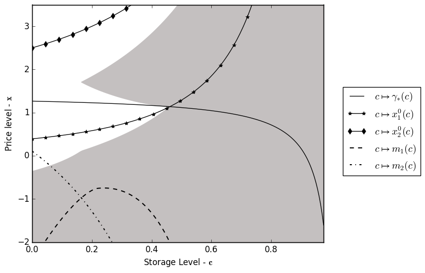
Refer to caption
Figure 1: An indicative example of an optimal entry region (shaded) when c^>1\hat{c}>1, together with the functions γ∗\gamma_{*} and x10x^{0}_{1}, x20x^{0}_{2} (introduced in Prop. 5.1 below). The functions m1m_{1} and m2m_{2} (not drawn to scale) are important determinants for the presence of the kinked shape (see Remark 5.4 below). This plot was generated using μ=1\mu=1, θ=1\theta=1, σ=3\sigma=3, λ=1\lambda=1, P0=4P_{0}=4 and Φ⁡(c)=2.2​(1−c)+8​(1−c)2\Phi(c)=2.2(1-c)+8(1-c)^{2}.

4.1 The case c^<0\hat{c}<0

Let us now assume that c^<0\hat{c}<0, i.e. k⁡(c)>0k(c)>0 for all c∈[0,1]c\in[0,1] (cf. (3.3)). We first recall from Section 2.2 of [7] that in this case

U⁡(x,c)=x⁡(1−c)−∫c1u⁡(x,y)​𝑑y,for (x,c)∈ℝ×[0,1],\displaystyle U(x,c)=x(1-c)-\int_{c}^{1}{u(x;y)dy},\qquad\text{for $(x,c)\in\mathbb{R}\times[0,1]$,} (4.2)

where uu is the value function of an associated optimal stopping problem with (cf. Sections 2.1 and 2.2 of [7])

(i)(i) u⁡(⋅,c)∈Wl​o​c2,∞​(ℝ)u(\,\cdot\,,c)\in W^{2,\infty}_{loc}(\mathbb{R}) for any c∈[0,1]c\in[0,1] (4.3)
(i​i)(ii) u⁡(x,c)>0u(x,c)>0 for x>β∗​(c)x>\beta_{*}(c) and u⁡(x,c)=0u(x,c)=0 for x≤β∗​(c)x\leq\beta_{*}(c), c∈[0,1],c\in[0,1], (4.4)

and with β∗\beta_{*} given as in Proposition 3.1-OPENi)i). Moreover, defining

G⁡(x,c):=μ⁡(k⁡(c)−θ)λ+k​(c)​(x−μ)λ+θ,\displaystyle G(x,c):=\frac{\mu(k(c)-\theta)}{\lambda}+\frac{k(c)(x-\mu)}{\lambda+\theta}, (4.5)

and recalling ϕλ\phi_{\lambda} from Definition 4.2, uu is expressed analytically as

u⁡(x,c)={G⁡(x,c)−G​(β∗​(c),c)ϕλ​(β∗​(c))​ϕλ​(x),x>β∗​(c)0,x≤β∗​(c)\displaystyle u(x,c)=\left\{\begin{array}[]{ll}G(x,c)-\frac{G({\beta_{*}(c)},c)}{\phi_{\lambda}({\beta_{*}(c)})}\phi_{\lambda}(x),&x>{\beta_{*}(c)}\\[4.0pt] 0,&x\leq{\beta_{*}(c)}\end{array}\right.

for c∈[0,1]c\in[0,1], and it solves the variational problem

(𝕃X−λ)​u​(x,c)=θ​μ−k⁡(c)​x\displaystyle\big(\mathbb{L}_{X}-\lambda\big)u(x,c)=\theta\mu-k(c)x x>β∗​(c),c∈[0,1]\displaystyle x>\beta_{*}(c),\,c\in[0,1] (4.8)
(𝕃X−λ)​u​(x,c)=0\displaystyle\big(\mathbb{L}_{X}-\lambda\big)u(x,c)=0 x≤β∗​(c),c∈[0,1]\displaystyle x\leq\beta_{*}(c),\,c\in[0,1] (4.9)
u⁡(β∗​(c),c)=ux​(β∗​(c),c)=0\displaystyle u(\beta_{*}(c),c)=u_{x}(\beta_{*}(c),c)=0 c∈[0,1].\displaystyle c\in[0,1]. (4.10)

By the regularity of uu and dominated convergence we have

(𝕃X−λ)​U​(x,c)=(1−c)​(θ​μ−(λ+θ)​x)−∫c1(𝕃X−λ)​u​(x,y)​𝑑y(\mathbb{L}_{X}-\lambda)U(x,c)=(1-c)(\theta\mu-(\lambda+\theta)x)-\int_{c}^{1}(\mathbb{L}_{X}-\lambda)u(x;y)dy (4.11)

for (x,c)∈ℝ×[0,1](x,c)\in\mathbb{R}\times[0,1].

As is usual, for each c∈[0,1]c\in[0,1] we define the continuation region 𝒞Vc\mathcal{C}^{c}_{V} and stopping region 𝒟Vc\mathcal{D}^{c}_{V} for the optimal stopping problem (3.15) as

𝒞Vc={x∈ℝ:V⁡(x,c)<U⁡(x,c)−P0},𝒟Vc={x∈ℝ:V⁡(x,c)=U⁡(x,c)−P0}.\displaystyle\mathcal{C}^{c}_{V}=\{x\in\mathbb{R}\,:\,V(x,c)<U(x,c)-P_{0}\}\,,\quad\mathcal{D}^{c}_{V}=\{x\in\mathbb{R}\,:\,V(x,c)=U(x,c)-P_{0}\}. (4.12)

With the aim of characterising the geometry of 𝒞Vc\mathcal{C}^{c}_{V} and 𝒟Vc\mathcal{D}^{c}_{V} we start by providing some preliminary results on U−P0U-P_{0} that will help to formulate an appropriate free-boundary problem for VV.

Proposition 4.1.

For any given c∈[0,1]c\in[0,1], there exists a unique x0​(c)∈ℝx^{0}(c)\in\mathbb{R} such that

(𝕃X−λ)​(U⁡(x,c)−P0)​{<0for x>x0​(c)=0for x=x0​(c)>0for x<x0​(c)\displaystyle\big(\mathbb{L}_{X}-\lambda\big)\big(U(x,c)-P_{0})\left\{\begin{array}[]{ll}<0&\text{for $x>x^{0}(c)$}\\[3.0pt] =0&\text{for $x=x^{0}(c)$}\\[3.0pt] >0&\text{for $x<x^{0}(c)$}\end{array}\right.

We refer to Appendix A for the proof of the previous proposition.

As discussed at the beginning of Section 4, it is never optimal in problem (3.15) to stop in (x0​(c),∞)(x^{0}(c),\infty), c∈[0,1]c\in[0,1], for x0​(c)x^{0}(c) as in Proposition 4.1, i.e.

(x0​(c),∞)⊆𝒞Vcfor c∈[0,1],\displaystyle(x^{0}(c),\infty)\subseteq\mathcal{C}^{c}_{V}\qquad\text{for $c\in[0,1]$,} (4.16)

and consequently

𝒟Vc⊂[−∞,x0​(c)]for c∈[0,1].\displaystyle\mathcal{D}^{c}_{V}\subset[-\infty,x^{0}(c)]\qquad\text{for $c\in[0,1]$.} (4.17)

Hence we conjecture that the optimal stopping strategy should be of single threshold type. In what follows we aim at finding ℓ∗​(c)\ell_{*}(c), c∈[0,1]c\in[0,1], such that 𝒟Vc=[−∞,ℓ∗​(c)]\mathcal{D}^{c}_{V}=[-\infty,\ell_{*}(c)] and

τ∗​(x,c)=inf{t≥0:Xtx≤ℓ∗​(c)}\displaystyle\tau^{*}(x,c)=\inf\{t\geq 0:X^{x}_{t}\leq\ell_{*}(c)\} (4.18)

is optimal for V⁡(x,c)V(x,c) in (3.15) with (x,c)∈ℝ×[0,1](x,c)\in\mathbb{R}\times[0,1]. The methodology adopted in [7, Sec. 2.1] does not apply directly to this problem due to the semi-explicit expression of the gain function U−P0U-P_{0}.

4.1.1 Formulation of Auxiliary Optimal Stopping Problems

To work out the optimal boundary ℓ∗\ell_{*} we will introduce auxiliary optimal stopping problems and employ a guess-and-verify approach in two frameworks with differing technical issues. We first observe that since UU is a classical solution of (3.5), an application of Dynkin’s formula to (3.15) provides a lower bound for VV, that is

V⁡(x,c)≥U⁡(x,c)−P0+Γ⁡(x,c),(x,c)∈ℝ×[0,1],\displaystyle V(x,c)\geq U(x,c)-P_{0}+\Gamma(x,c),\qquad(x,c)\in\mathbb{R}\times[0,1], (4.19)

with

Γ⁡(x,c):=infτ≥0𝖤⁡[∫0τe−λ​s​(λ​P0−λ​Xsx​Φ​(c))​𝑑s](x,c)∈ℝ×[0,1].\displaystyle\Gamma(x,c):=\inf_{\tau\geq 0}\mathsf{E}\bigg[\int_{0}^{\tau}e^{-\lambda s}\big(\lambda P_{0}-\lambda X^{x}_{s}\Phi(c)\big)ds\bigg]\qquad(x,c)\in\mathbb{R}\times[0,1]. (4.20)

On the other hand, for (x,c)∈ℝ×[0,1](x,c)\in\mathbb{R}\times[0,1] fixed, set σβ∗:=inf{t≥0:Xtx≤β∗​(c)}\sigma^{*}_{\beta}:=\inf\{t\geq 0\,:\,X^{x}_{t}\leq\beta_{*}(c)\} with β∗\beta_{*} as in Proposition 3.1, then for arbitrary stopping time τ\tau one also obtains

𝖤\displaystyle\mathsf{E} [e−λ⁡(τ∧σβ∗)​(U⁡(Xτ∧σβ∗x,c)−P0)]\displaystyle\Big[e^{-\lambda(\tau\wedge\sigma^{*}_{\beta})}\Big(U(X^{x}_{\tau\wedge\sigma^{*}_{\beta}},c)-P_{0}\Big)\Big] (4.21)
=U⁡(x,c)−P0+𝖤⁡[∫0τ∧σβ∗e−λ​s​(λ​P0−λ​Xsx​Φ​(c))​𝑑s]\displaystyle=U(x,c)-P_{0}+\mathsf{E}\bigg[\int_{0}^{\tau\wedge\sigma^{*}_{\beta}}e^{-\lambda s}\big(\lambda P_{0}-\lambda X^{x}_{s}\Phi(c)\big)ds\bigg]

by using the fact that UU solves (3.5) and Dynkin’s formula. We can now obtain an upper bound for VV by setting

Γβ​(x,c):=infτ≥0𝖤⁡[∫0τ∧σβ∗e−λ​s​(λ​P0−λ​Xsx​Φ​(c))​𝑑s],(x,c)∈ℝ×[0,1],\displaystyle\Gamma_{\beta}(x,c):=\inf_{\tau\geq 0}\mathsf{E}\bigg[\int_{0}^{\tau\wedge\sigma^{*}_{\beta}}e^{-\lambda s}\big(\lambda P_{0}-\lambda X^{x}_{s}\Phi(c)\big)ds\bigg],\quad(x,c)\in\mathbb{R}\times[0,1], (4.22)

so that taking the infimum over all τ\tau in (4.21) one obtains

V⁡(x,c)\displaystyle V(x,c) ≤U⁡(x,c)−P0+Γβ​(x,c)(x,c)∈ℝ×[0,1].\displaystyle\leq U(x,c)-P_{0}+\Gamma_{\beta}(x,c)\qquad(x,c)\in\mathbb{R}\times[0,1]. (4.23)

It turns out that (4.19) and (4.23) allow us to find a simple characterisation of the optimal boundary ℓ∗\ell_{*} and of the function VV in some cases. Let us first observe that 0≥Γβ​(x,c)≥Γ⁡(x,c)0\geq\Gamma_{\beta}(x,c)\geq\Gamma(x,c) for all (x,c)∈ℝ×[0,1](x,c)\in\mathbb{R}\times[0,1]. Defining for each fixed c∈[0,1]c\in[0,1] the stopping regions

𝒟Γc={x∈ℝ:Γ⁡(x,c)=0}and𝒟Γβc={x∈ℝ:Γβ​(x,c)=0}\displaystyle\mathcal{D}^{c}_{\Gamma}=\{x\in\mathbb{R}\,:\,\Gamma(x,c)=0\}\qquad\text{and}\qquad\mathcal{D}^{c}_{\Gamma_{\beta}}=\{x\in\mathbb{R}\,:\,\Gamma_{\beta}(x,c)=0\}

it is easy to see that 𝒟Γc⊂𝒟Γβc\mathcal{D}^{c}_{\Gamma}\subset\mathcal{D}^{c}_{\Gamma_{\beta}}. Moreover, by the monotonicity of x↦X⋅xx\mapsto X^{x}_{\cdot} it is not hard to verify that x↦Γ⁡(x,c)x\mapsto\Gamma(x,c) and x↦Γβ​(x,c)x\mapsto\Gamma_{\beta}(x,c) are decreasing. Hence we again expect optimal stopping strategies of threshold type, i.e.

𝒟Γc={x∈ℝ:x≤α1∗​(c)}and𝒟Γβc={x∈ℝ:x≤α2∗​(c)}\displaystyle\mathcal{D}^{c}_{\Gamma}=\{x\in\mathbb{R}\,:\,x\leq\alpha^{*}_{1}(c)\}\qquad\text{and}\qquad\mathcal{D}^{c}_{\Gamma_{\beta}}=\{x\in\mathbb{R}\,:\,x\leq\alpha^{*}_{2}(c)\} (4.24)

for c∈[0,1]c\in[0,1] and for suitable functions αi∗​(⋅)\alpha^{*}_{i}(\,\cdot\,), i=1,2i=1,2 to be determined.

Assume for now that α1∗\alpha^{*}_{1} and α2∗\alpha^{*}_{2} are indeed optimal, then we must have

α1∗​(c)≤ℓ∗​(c)≤α2∗​(c)for c∈[0,1].\displaystyle\alpha^{*}_{1}(c)\leq\ell_{*}(c)\leq\alpha_{2}^{*}(c)\qquad\text{for $c\in[0,1]$}. (4.25)

Indeed, for all (x,c)∈ℝ×[0,1](x,c)\in\mathbb{R}\times[0,1] we have 𝒟Γc⊂𝒟Vc\mathcal{D}^{c}_{\Gamma}\subset\mathcal{D}^{c}_{V} since Γ⁡(x,c)≤V⁡(x,c)−U⁡(x,c)+P0≤0\Gamma(x,c)\leq V(x,c)-U(x,c)+P_{0}\leq 0, and 𝒟Vc⊂𝒟Γβc\mathcal{D}^{c}_{V}\subset\mathcal{D}^{c}_{\Gamma_{\beta}} since V⁡(x,c)−U⁡(x,c)+P0≤Γβ​(x,c)≤0V(x,c)-U(x,c)+P_{0}\leq\Gamma_{\beta}(x,c)\leq 0. Notice also that since the optimisation problem in (4.22) is the same as the one in (4.20) except that in the former the observation is stopped when XX hits β∗\beta_{*}, we must have

α2∗​(c)=β∗​(c)∨α1∗​(c)for​c∈[0,1].\alpha^{*}_{2}(c)=\beta_{*}(c)\vee\alpha_{1}^{*}(c)\quad\text{for}\enskip c\in[0,1]. (4.26)

Thus for each c∈[0,1]c\in[0,1] we can now consider two cases:

  1. 1.

    if α1∗​(c)>β∗​(c)\alpha_{1}^{*}(c)>\beta_{*}(c) we have Γ⁡(x,c)=Γβ​(x,c)=(V−U+P0)​(x,c)\Gamma(x,c)=\Gamma_{\beta}(x,c)=\big(V-U+P_{0}\big)(x,c) for x∈ℝx\in\mathbb{R} and ℓ∗​(c)=α1∗​(c)\ell_{*}(c)=\alpha_{1}^{*}(c),

  2. 2.

    if α1∗​(c)≤β∗​(c)\alpha_{1}^{*}(c)\leq\beta_{*}(c) we have α2∗​(c)=β∗​(c)\alpha^{*}_{2}(c)=\beta_{*}(c), implying that ℓ∗​(c)≤β∗​(c)\ell_{*}(c)\leq\beta_{*}(c).

Both 1.1. and 2.2. above need to be studied in order to obtain a complete characterisation of ℓ∗\ell_{*}, however we note that case 1.1. is particularly interesting as it identifies VV and ℓ∗\ell_{*} with Γ+U−P0\Gamma+U-P_{0} and α1∗\alpha^{*}_{1}, respectively. As we will clarify in what follows, solving problem (4.20) turns out to be theoretically simpler and computationally less demanding than dealing directly with problem (3.15).

4.1.2 Solution of the Auxiliary Optimal Stopping Problems

To make our claims rigorous we start by analysing problem (4.20). This is accomplished by largely relying on arguments already employed in [7, Sec. 2.1] and therefore we omit proofs here whenever a precise reference can be provided. Moreover, the majority of the proofs of new results are provided in Appendix A to simplify the exposition. Let us now introduce two functions ϕλ\phi_{\lambda} and ψλ\psi_{\lambda} which feature frequently below.

Definition 4.2.

Let ϕλ:ℝ→ℝ+\phi_{\lambda}:\mathbb{R}\to\mathbb{R}^{+} and ψλ:ℝ→ℝ+\psi_{\lambda}:\mathbb{R}\to\mathbb{R}^{+} denote respectively the decreasing and increasing fundamental solutions of the differential equation 𝕃X​f=λ​f\mathbb{L}_{X}f=\lambda f on ℝ\mathbb{R} (see Appendix B for details).

In problem (4.20) we conjecture an optimal stopping time of the form

τα​(x,c):=inf{t≥0:Xtx≤α⁡(c)}\displaystyle\tau_{\alpha}(x,c):=\inf\{t\geq 0\,:\,X^{x}_{t}\leq\alpha(c)\} (4.27)

for (x,c)∈ℝ×[0,1](x,c)\in\mathbb{R}\times[0,1] and α\alpha to be determined. Under this conjecture Γ\Gamma should be found in the class of functions of the form

Γα​(x,c)={𝖤⁡[∫0ταe−λ​s​λ​(P0−Xsx​Φ​(c))​ds],x>α⁡(c)0,x≤α⁡(c)\Gamma^{\alpha}(x,c)=\left\{\begin{array}[]{ll}\displaystyle\mathsf{E}\bigg[\int_{0}^{\tau_{\alpha}}e^{-\lambda s}\lambda\big(P_{0}-X^{x}_{s}\Phi(c)\big)ds\bigg],&x>\alpha(c)\\[3.0pt] 0,&x\leq\alpha(c)\end{array}\right. (4.28)

for each c∈[0,1]c\in[0,1]. Now, repeating the same arguments of proof of [7, Thm. 2.1] we obtain

Lemma 4.3.

One has

Γα​(x,c)={(P0−G^​(x,c))−(P0−G^​(α⁡(c),c))​ϕλ​(x)ϕλ​(α​(c)),x>α⁡(c)0,x≤α⁡(c)\displaystyle\Gamma^{\alpha}(x,c)=\left\{\begin{array}[]{ll}\big(P_{0}-\hat{G}(x,c)\big)-\big(P_{0}-\hat{G}(\alpha(c),c)\big)\frac{\phi_{\lambda}(x)}{\phi_{\lambda}(\alpha(c))},&x>\alpha(c)\\[5.0pt] 0,&x\leq\alpha(c)\end{array}\right.

for each c∈[0,1]c\in[0,1], with

G^​(x,c):=μ​Φ​(c)+(x−μ)​λ​Φ​(c)λ+θ(x,c)∈ℝ×[0,1].\displaystyle\hat{G}(x,c):=\mu\Phi(c)+(x-\mu)\tfrac{\lambda\Phi(c)}{\lambda+\theta}\qquad(x,c)\in\mathbb{R}\times[0,1]. (4.31)

To single out the candidate optimal boundary we impose the so-called smooth fit condition, i.e. dd​x​Γα​(α⁡(c),c)=0\tfrac{d}{dx}\Gamma^{\alpha}(\alpha(c),c)=0 for every c∈[0,1]c\in[0,1]. This amounts to finding α∗\alpha^{*} such that

−λ​Φ​(c)λ+θ+(G^​(α∗​(c),c)−P0)​ϕλ′​(α∗​(c))ϕλ​(α∗​(c))=0for c∈[0,1].\displaystyle-\tfrac{\lambda\Phi(c)}{\lambda+\theta}+\big(\hat{G}(\alpha^{*}(c),c)-P_{0}\big)\tfrac{\phi^{\prime}_{\lambda}(\alpha^{*}(c))}{\phi_{\lambda}(\alpha^{*}(c))}=0\quad\text{for $c\in[0,1]$}. (4.32)
Proposition 4.4.

For c∈[0,1]c\in[0,1] define

x0†​(c):=μ+(P0−μ​Φ​(c))​(λ+θ)λ​Φ​(c).\displaystyle x^{\dagger}_{0}(c):=\mu+\big(P_{0}-\mu\Phi(c)\big)\tfrac{(\lambda+\theta)}{\lambda\Phi(c)}. (4.33)

For each c∈[0,1]c\in[0,1] there exists a unique solution α∗​(c)∈(−∞,x0†​(c))\alpha^{*}(c)\in(-\infty,x^{\dagger}_{0}(c)) of (4.32). Moreover α∗∈C1​([0,1))\alpha^{*}\in C^{1}([0,1)) and it is strictly increasing with limc→1α∗​(c)=+∞\lim_{c\to 1}\alpha^{*}(c)=+\infty.

For the proof of Proposition 4.4 we refer to Appendix A.

To complete the characterisation of α∗\alpha^{*} and Γα∗\Gamma^{\alpha^{*}} we now find an alternative upper bound for α∗\alpha^{*} that will guarantee (𝕃X​Γα∗−λ​Γα∗)​(x,c)≥−λ⁡(P0−x​Φ​(c))\big(\mathbb{L}_{X}\Gamma^{\alpha^{*}}-\lambda\Gamma^{\alpha^{*}}\big)(x,c)\geq-\lambda(P_{0}-x\Phi(c)) for (x,c)∈ℝ×[0,1](x,c)\in\mathbb{R}\times[0,1]. Again, the proof of the following result may be found in Appendix A.

Proposition 4.5.

For all c∈[0,1]c\in[0,1] we have α∗​(c)≤P0/Φ⁡(c)\alpha^{*}(c)\leq P_{0}/\Phi(c) with α∗\alpha^{*} as in Proposition 4.4.

With the aim of formulating a variational problem for Γα∗\Gamma^{\alpha^{*}} we observe that d2d​x2​Γα∗​(x,c)>0\tfrac{d^{2}}{dx^{2}}\Gamma^{\alpha^{*}}(x,c)>0 for x>α∗​(c)x>\alpha^{*}(c), c∈[0,1]c\in[0,1] by (4.3), convexity of ϕλ\phi_{\lambda} and the fact that G^​(α∗​(c),c)−P0<0\hat{G}(\alpha^{*}(c),c)-P_{0}<0. Hence Γα∗≥0\Gamma^{\alpha^{*}}\geq 0 on ℝ×[0,1]\mathbb{R}\times[0,1]. It is not hard to verify by direct calculation from (4.3) and the above results that for all c∈[0,1]c\in[0,1] the couple (Γα∗​(⋅,c),α∗​(c))\big(\Gamma^{\alpha^{*}}(\,\cdot\,,c),\alpha^{*}(c)\big) solves the free-boundary problem

(𝕃X−λ)​Γα∗​(x,c)=−λ⁡(P0−x​Φ​(c))\displaystyle\big(\mathbb{L}_{X}-\lambda\big)\Gamma^{\alpha^{*}}(x,c)=-\lambda(P_{0}-x\Phi(c)) x>α∗​(c),\displaystyle x>{\alpha^{*}}(c), (4.34)
(𝕃X−λ)​Γα∗​(x,c)>−λ⁡(P0−x​Φ​(c))\displaystyle\big(\mathbb{L}_{X}-\lambda\big)\Gamma^{\alpha^{*}}(x,c)>-\lambda(P_{0}-x\Phi(c)) x<α∗​(c),\displaystyle x<\alpha^{*}(c), (4.35)
Γα∗​(α∗​(c),c)=Γxα∗​(α∗​(c),c)=0,Γα∗​(x,c)≥0\displaystyle\Gamma^{\alpha^{*}}(\alpha^{*}(c),c)=\Gamma^{\alpha^{*}}_{x}(\alpha^{*}(c),c)=0,\quad\Gamma^{\alpha^{*}}(x,c)\geq 0 x∈ℝ\displaystyle x\in\mathbb{R} (4.36)

and Γα∗​(⋅,c)∈Wl​o​c2,∞​(ℝ)\Gamma^{\alpha^{*}}(\,\cdot\,,c)\in W^{2,\infty}_{loc}(\mathbb{R}). Following now the same arguments as in the proof of [7, Thm. 2.1], which is based on an application of the Itô-Tanaka formula and (4.34)–(4.36), we can verify our guess and prove the following theorem (the details are omitted).

Theorem 4.6.

The boundary α∗\alpha^{*} of Proposition 4.4 is optimal for (4.20) in the sense that α∗=α1∗\alpha^{*}=\alpha^{*}_{1} with α1∗\alpha^{*}_{1} as in (4.24),

τα∗=inf{t≥0:Xtx≤α∗​(c)}\displaystyle\tau^{*}_{\alpha}=\inf\{t\geq 0\,:\,X^{x}_{t}\leq{\alpha_{*}(c)}\} (4.37)

is an optimal stopping time and Γα∗≡Γ\Gamma^{\alpha^{*}}\equiv\Gamma (cf. (4.20)).

4.1.3 Solution of the Original Optimal Stopping Problem (3.15)

In Theorem 4.6 we have fully characterised α1∗\alpha^{*}_{1} and Γ\Gamma thus also α2∗\alpha^{*}_{2} and Γβ\Gamma_{\beta} (cf. (4.22), (4.24) and (4.26)). Moreover we have found that α1∗​(⋅)\alpha^{*}_{1}(\,\cdot\,) is strictly increasing on [0,1)[0,1). On the other hand, β∗​(⋅)\beta_{*}(\,\cdot\,) is a strictly decreasing function (cf. Proposition 3.1-OPENi)i)), hence there exists at most one c∗∈(0,1)c_{*}\in(0,1) such that

β∗​(c)>α1∗​(c) for c∈(0,c∗) and β∗​(c)≤α1∗​(c) for c∈[c∗,1).\displaystyle\text{$\beta_{*}(c)>\alpha^{*}_{1}(c)$ for $c\in(0,c_{*})$ and $\beta_{*}(c)\leq\alpha^{*}_{1}(c)$ for $c\in[c_{*},1)$}. (4.38)

As already mentioned, it may be possible to provide examples where such a value c∗c_{*} does not exist (0,1)(0,1) and α1∗​(c)>β∗​(c)\alpha^{*}_{1}(c)>\beta_{*}(c) for all c∈[0,1]c\in[0,1]. In those cases, as discussed in Section 4.1.1, one has ℓ∗=α1∗\ell_{*}=\alpha^{*}_{1} and V=U−P0+ΓV=U-P_{0}+\Gamma and problem (3.15) is fully solved. Therefore to provide a complete analysis of problem (3.15) we must consider the case when c∗c_{*} exists in (0,1)(0,1). From now on we make the following assumption.

Assumption 4.7.

There exists a unique c∗∈(0,1)c_{*}\in(0,1) such that (4.38) holds.

As a consequence of the analysis in Section 4.1.2 we have the next simple corollary.

Corollary 4.8.

For all c∈[c∗,1)c\in[c_{*},1) it holds V⁡(x,c)=(Γ+U−P0)​(x,c)V(x,c)=(\Gamma+U-P_{0})(x,c), x∈ℝx\in\mathbb{R} and ℓ∗​(c)=α1∗​(c)\ell_{*}(c)=\alpha^{*}_{1}(c), with Γ\Gamma and α1∗\alpha^{*}_{1} as in Theorem 4.6.

It remains to characterise ℓ∗\ell_{*} in the interval [0,c∗)[0,c_{*}) in which we have ℓ∗​(c)≤β∗​(c)\ell_{*}(c)\leq\beta_{*}(c). This is done in Theorem 4.13, whose proof requires other technical results which are cited here and proved in the appendix. Fix c∈[0,c∗)c\in[0,c_{*}), let ℓ⁡(c)∈ℝ\ell(c)\in\mathbb{R} be a candidate boundary and define the stopping time τℓ​(x,c):=inf{t≥0:Xtx≤ℓ⁡(c)}\tau_{\ell}(x,c):=\inf\big\{t\geq 0\,:\,X^{x}_{t}\leq\ell(c)\big\} for x∈ℝx\in\mathbb{R}. Again to simplify notation we set τℓ=τℓ​(x,c)\tau_{\ell}=\tau_{\ell}(x,c) when no confusion may arise. It is now natural to associate to ℓ⁡(c)\ell(c) a candidate value function

Vℓ​(x,c):=𝖤⁡[e−λ​τℓ​(U⁡(Xτℓx,c)−P0)],\displaystyle V^{\ell}(x,c):=\mathsf{E}\left[e^{-\lambda\tau_{\ell}}\Big(U(X^{x}_{\tau_{\ell}},c)-P_{0}\Big)\right], (4.39)

whose analytical expression is provided in the next lemma.

Lemma 4.9.

For c∈[0,c∗)c\in[0,c_{*}) we have

Vℓ​(x,c)={(U⁡(ℓ⁡(c),c)−P0)​ϕλ​(x)ϕλ​(ℓ​(c)),x>ℓ⁡(c)U⁡(x,c)−P0,x≤ℓ⁡(c)\displaystyle V^{\ell}(x,c)=\left\{\begin{array}[]{ll}(U(\ell(c),c)-P_{0})\frac{\phi_{\lambda}(x)}{\phi_{\lambda}(\ell(c))},&x>\ell(c)\\[4.0pt] U(x,c)-P_{0},&x\leq\ell(c)\end{array}\right.

The candidate boundary ℓ∗\ell_{*}, whose optimality will be subsequently verified, is found by imposing the smooth fit condition, i.e.

(U⁡(ℓ∗​(c),c)−P0)​ϕλ′​(ℓ∗​(c))ϕλ​(ℓ∗​(c))=Ux​(ℓ∗​(c),c),c∈[0,1].\displaystyle(U(\ell_{*}(c),c)-P_{0})\frac{\phi^{\prime}_{\lambda}(\ell_{*}(c))}{\phi_{\lambda}(\ell_{*}(c))}=U_{x}(\ell_{*}(c),c),\qquad c\in[0,1]. (4.42)
Proposition 4.10.

For any c∈[0,c∗)c\in[0,c_{*}) there exists at least one solution ℓ∗​(c)∈(−∞,x0​(c))\ell_{*}(c)\in(-\infty,x^{0}(c)) of (4.42) with x0​(c)x^{0}(c) as in Proposition 4.1.

Remark 4.11.

A couple of remarks before we proceed.

i. The analytical representation (4.9) in fact holds for all c∈[0,1]c\in[0,1] and it must coincide with (4.3) for c∈[c∗,1]c\in[c_{*},1]. Furthermore, the optimal boundary α1∗\alpha^{*}_{1} found in Section 4.1.2 by solving (4.32) must also solve (4.42) for all c∈[c∗,1]c\in[c_{*},1] since α1∗=ℓ∗\alpha^{*}_{1}=\ell_{*} on that set. This equivalence can be verified by comparing numerical solutions to (4.32) and (4.42). Finding a numerical solution to (4.42) for c∈[0,c∗)c\in[0,c_{*}) (if it exists) is computationally more demanding than solving (4.32), however, because of the absence of an explicit expression of the function UU.

ii. It is important to observe that the proof of Proposition 4.10 does not use that c∈[0,c∗)c\in[0,c_{*}) and in fact it holds for c∈[0,1]c\in[0,1]. However, arguing as in Section 4.1.2 we managed to obtain further regularity properties of the optimal boundary in [c∗,1][c_{*},1] and its uniqueness. We shall see in what follows that uniqueness can be retrieved also in c∈[0,c∗)c\in[0,c_{*}) but it requires a deeper analysis.

Now that the existence of at least one candidate optimal boundary ℓ∗\ell_{*} has been established, for the purpose of performing a verification argument we would also like to establish that for arbitrary c∈[0,c∗)c\in[0,c_{*}) we have Vℓ∗​(x,c)≤U⁡(x,c)−P0V^{\ell_{*}}(x,c)\leq U(x,c)-P_{0}, x∈ℝx\in\mathbb{R}. This is verified in the following proposition (whose proof is collected in appendix).

Proposition 4.12.

For c∈[0,c∗)c\in[0,c_{*}) and for any ℓ∗\ell_{*} solving (4.42) it holds Vℓ∗​(x,c)≤U⁡(x,c)−P0V^{\ell_{*}}(x,c)\leq U(x,c)-P_{0}, x∈ℝx\in\mathbb{R}.

Finally we provide a verification theorem establishing the optimality of our candidate boundary ℓ∗\ell_{*} and, as a by-product, also implying uniqueness of the solution to (4.42).

Theorem 4.13.

There exists a unique solution of (4.42) in (−∞,x0(c¯)](-\infty,x^{0}(\bar{c})]. This solution is the optimal boundary of problem (3.15) in the sense that Vℓ∗=VV^{\ell_{*}}=V on ℝ×[0,1)\mathbb{R}\times[0,1) (cf. (4.9)) and the stopping time

τ∗:=τℓ∗​(x,c)=inf{t≥0:Xtx≤ℓ∗​(c)}\displaystyle\tau^{*}:=\tau^{*}_{\ell}(x,c)=\inf\{t\geq 0\,:\,X^{x}_{t}\leq\ell_{*}(c)\} (4.43)

is optimal in (3.15) for all (x,c)∈ℝ×[0,1)(x,c)\in\mathbb{R}\times[0,1).

Proof.

For c∈[c∗,1)c\in[c_{*},1) the proof was provided in Section 4.1.2 recalling that ℓ∗=α1∗\ell_{*}=\alpha^{*}_{1} on [c∗,1)[c_{*},1) and V=U−P0+ΓV=U-P_{0}+\Gamma on ℝ×[c∗,1)\mathbb{R}\times[c_{*},1) (cf. (4.20), Remark 4.11). For c∈[0,c∗)c\in[0,c_{*}) we split the proof into two parts.

1.1. Optimality. Fix c¯∈[0,c∗)\bar{c}\in[0,c_{*}). Here we prove that if ℓ∗​(c¯)\ell_{*}(\bar{c}) is any solution of (4.42) then Vℓ∗​(⋅,c¯)=V⁡(⋅,c¯)V^{\ell_{*}}(\,\cdot\,,\bar{c})=V(\,\cdot\,,\bar{c}) on ℝ\mathbb{R} (cf. (3.15) and (4.9)).

First we note that Vℓ∗​(⋅,c¯)≥V⁡(⋅,c¯)V^{\ell_{*}}(\,\cdot\,,\bar{c})\geq V(\,\cdot\,,\bar{c}) on ℝ\mathbb{R} by (3.15) and (4.39). To obtain the reverse inequality we will rely on Itô-Tanaka’s formula. Observe that Vℓ∗​(⋅,c¯)∈C1​(ℝ)V^{\ell_{*}}(\,\cdot\,,\bar{c})\in C^{1}(\mathbb{R}) by (4.9) and (4.42), and Vx​xℓ∗​(⋅,c¯)V^{\ell_{*}}_{xx}(\,\cdot\,,\bar{c}) is continuous on ℝ∖{ℓ∗​(c¯)}\mathbb{R}\setminus\big\{\ell_{*}(\bar{c})\big\} and bounded at the boundary ℓ∗​(c¯)\ell_{*}(\bar{c}). Moreover from (4.9) we get

(𝕃X−λ)​Vℓ∗​(x,c¯)=0\displaystyle\big(\mathbb{L}_{X}-\lambda\big)V^{\ell_{*}}(x,\bar{c})=0 for x>ℓ∗​(c¯)x>\ell_{*}(\bar{c}) (4.44)
(𝕃X−λ)​Vℓ∗​(x,c¯)=(𝕃X−λ)​(U−P0)​(x,c¯)>0\displaystyle\big(\mathbb{L}_{X}-\lambda\big)V^{\ell_{*}}(x,\bar{c})=\big(\mathbb{L}_{X}-\lambda\big)(U-P_{0})(x,\bar{c})>0 for x≤ℓ∗​(c¯)x\leq\ell_{*}(\bar{c}) (4.45)

where the inequality in (4.45) holds by (4.1) since ℓ∗​(c¯)≤x0​(c¯)\ell_{*}(\bar{c})\leq x^{0}(\bar{c}) (cf. Proposition 4.10). An application of Itô-Tanaka’s formula (see [17], Chapter 3, Problem 6.24, p. 215), (4.44), (4.45) and Proposition 4.12 give

Vℓ∗​(x,c¯)\displaystyle V^{\ell_{*}}(x,\bar{c}) =𝖤⁡[e−λ⁡(τ∧τR)​Vℓ∗​(Xτ∧τRx,c¯)−∫0τ∧τRe−r​t​(𝕃X−λ)​Vℓ∗​(Xtx,c¯)​𝑑t]\displaystyle=\mathsf{E}\left[e^{-\lambda(\tau\wedge\tau_{R})}V^{\ell_{*}}\big(X^{x}_{\tau\wedge\tau_{R}},\bar{c}\big)-\int_{0}^{\tau\wedge\tau_{R}}{e^{-rt}}\big(\mathbb{L}_{X}-\lambda\big)V^{\ell_{*}}(X^{x}_{t},\bar{c})dt\right] (4.46)
≤𝖤⁡[e−λ⁡(τ∧τR)​(U⁡(Xτ∧τRx,c¯)−P0)]\displaystyle\leq\mathsf{E}\left[e^{-\lambda(\tau\wedge\tau_{R})}\Big(U\big(X^{x}_{\tau\wedge\tau_{R}},\bar{c}\big)-P_{0}\Big)\right]

with τ\tau an arbitrary stopping time and τR:=inf{t≥0:|Xtx|≥R}\tau_{R}:=\inf\big\{t\geq 0\,:\,|X^{x}_{t}|\geq R\big\}, R>0R>0. We now pass to the limit as R→∞R\to\infty and recall that |U⁡(x,c¯)|≤C⁡(1+|x|)|U(x,\bar{c})|\leq C(1+|x|) (cf. Proposition 3.1) and that {e−λ​τR​|XτRx|,R>0}\big\{e^{-\lambda\tau_{R}}|X^{x}_{\tau_{R}}|\,,\,R>0\big\} is a uniformly integrable family (cf. Lemma B.2 in Appendix B). Then in the limit we use the dominated convergence theorem and the fact that

limR→∞e−λ⁡(τ∧τR)​Xτ∧τRx=e−λ​τ​Xτx,𝖯−a.s.\displaystyle\lim_{R\to\infty}e^{-\lambda(\tau\wedge\tau_{R})}X^{x}_{\tau\wedge\tau_{R}}=e^{-\lambda\tau}X^{x}_{\tau},\qquad\mathsf{P}-a.s.

to obtain Vℓ∗​(⋅,c¯)≤V⁡(⋅,c¯)V^{\ell_{*}}(\,\cdot\,,\bar{c})\leq V(\,\cdot\,,\bar{c}) on ℝ\mathbb{R} by the arbitrariness of τ\tau, hence Vℓ∗​(⋅,c¯)=V⁡(⋅,c¯)V^{\ell_{*}}(\,\cdot\,,\bar{c})=V(\,\cdot\,,\bar{c}) on ℝ\mathbb{R} and optimality of ℓ∗​(c¯)\ell_{*}(\bar{c}) follows.

2.2. Uniqueness. Here we prove the uniqueness of the solution of (4.42) via probabilistic arguments similar to those employed for the first time in [20]. Let c¯∈[0,c∗)\bar{c}\in[0,c_{*}) be fixed and, arguing by contradiction, let us assume that there exists another solution ℓ′​(c¯)≠ℓ∗​(c¯)\ell^{\prime}(\bar{c})\neq\ell_{*}(\bar{c}) of (4.42) with ℓ′​(c¯)≤x0​(c¯)\ell^{\prime}(\bar{c})\leq x^{0}(\bar{c}). Then by (3.15) and (4.39) it follows that

Vℓ′​(⋅,c¯)≥V⁡(⋅,c¯)=Vℓ∗​(⋅,c¯) on ℝ,\displaystyle V^{\ell^{\prime}}(\,\cdot\,,\bar{c})\geq V(\,\cdot\,,\bar{c})=V^{\ell_{*}}(\,\cdot\,,\bar{c})\qquad\text{ on $\mathbb{R}$,} (4.47)

Vℓ′​(⋅,c¯)∈C1​(ℝ)V^{\ell^{\prime}}(\,\cdot\,,\bar{c})\in C^{1}(\mathbb{R}) and Vx​xℓ′​(⋅,c¯)∈Ll​o​c∞​(ℝ)V^{\ell^{\prime}}_{xx}(\,\cdot\,,\bar{c})\in L^{\infty}_{loc}(\mathbb{R}) by the same arguments as in 1.1. above. By construction Vℓ′V^{\ell^{\prime}} solves (4.44) and (4.45) with ℓ∗\ell_{*} replaced by ℓ′\ell^{\prime}.

Assume for example that ℓ′​(c¯)<ℓ∗​(c¯)\ell^{\prime}(\bar{c})<\ell_{*}(\bar{c}), take x<ℓ′​(c¯)x<\ell^{\prime}(\bar{c}) and set σℓ∗:=inf{t≥0:Xtx≥ℓ∗​(c¯)}\sigma^{*}_{\ell}:=\inf\big\{t\geq 0\,:\,X^{x}_{t}\geq\ell_{*}(\bar{c})\big\}, then an application of Itô-Tanaka’s formula gives (up to a localisation argument as in 1.1. above)

𝖤⁡[e−λ​σℓ∗​Vℓ′​(Xσℓ∗x,c¯)]\displaystyle\mathsf{E}\left[e^{-\lambda\sigma_{\ell}^{*}}V^{\ell^{\prime}}\big(X^{x}_{\sigma^{*}_{\ell}},\bar{c}\big)\right] =Vℓ′​(x,c¯)+𝖤⁡[∫0σℓ∗e−λ​t​(𝕃X−λ)​Vℓ′​(Xtx,c¯)​𝑑t]\displaystyle=V^{\ell^{\prime}}(x,\bar{c})+\mathsf{E}\Big[\int^{\sigma^{*}_{\ell}}_{0}{e^{-\lambda t}\big(\mathbb{L}_{X}-\lambda\big)V^{\ell^{\prime}}\big(X^{x}_{t},\bar{c}\big)dt}\Big] (4.48)
=Vℓ′(x,c¯)+𝖤[∫0σℓ∗e−λ​t(𝕃X−λ)(U(Xtx,c¯)−P0)𝟙{Xxt<ℓ′(c¯)}dt]\displaystyle=V^{\ell^{\prime}}(x,\bar{c})+\mathsf{E}\Big[\int^{\sigma^{*}_{\ell}}_{0}{e^{-\lambda t}\big(\mathbb{L}_{X}-\lambda\big)\big(U\big(X^{x}_{t},\bar{c}\big)-P_{0}\big)\mathds{1}_{\{X^{x}_{t}<\ell^{\prime}(\bar{c})\}}dt}\Big]

and

𝖤⁡[e−λ​σℓ∗​V​(Xσℓ∗x,c¯)]\displaystyle\mathsf{E}\left[e^{-\lambda\sigma^{*}_{\ell}}V\big(X^{x}_{\sigma^{*}_{\ell}},\bar{c}\big)\right] =V⁡(x,c¯)+𝖤⁡[∫0σℓ∗e−λ​t​(𝕃X−λ)​(U⁡(Xtx,c¯)−P0)​𝑑t].\displaystyle=V(x,\bar{c})+\mathsf{E}\Big[\int^{\sigma^{*}_{\ell}}_{0}{e^{-\lambda t}\big(\mathbb{L}_{X}-\lambda\big)\big(U\big(X^{x}_{t},\bar{c}\big)-P_{0}\big)dt}\Big]. (4.49)

Recall that Vℓ′​(Xσℓ∗x,c¯)≥V⁡(Xσℓ∗x,c¯)V^{\ell^{\prime}}(X^{x}_{\sigma^{*}_{\ell}},\bar{c})\geq V(X^{x}_{\sigma^{*}_{\ell}},\bar{c}) by (4.47) and that for x<ℓ′​(c¯)≤ℓ∗​(c¯)x<\ell^{\prime}(\bar{c})\leq\ell_{*}(\bar{c}) one has V⁡(x,c¯)=Vℓ′​(x,c¯)=U⁡(x,c¯)−P0V(x,\bar{c})=V^{\ell^{\prime}}(x,\bar{c})=U(x,\bar{c})-P_{0}, hence subtracting (4.49) from (4.48) we get

−𝖤[∫0σℓ∗e−λ​t(𝕃X−λ)(U(Xtx,c¯)−P0)𝟙{ℓ′(c¯)<Xxt<ℓ∗(c¯)}dt]≥0.\displaystyle-\mathsf{E}\left[\int^{\sigma^{*}_{\ell}}_{0}{e^{-\lambda t}\big(\mathbb{L}_{X}-\lambda\big)\big(U\big(X^{x}_{t},\bar{c}\big)-P_{0}\big)\mathds{1}_{\{\ell^{\prime}(\bar{c})<X^{x}_{t}<\ell_{*}(\bar{c})\}}dt}\right]\geq 0. (4.50)

By the continuity of paths of XxX^{x} we must have σℓ∗>0\sigma^{*}_{\ell}>0, 𝖯\mathsf{P}-a.s. and since the law of XX is absolutely continuous with respect to the Lebesgue measure we also have 𝖯({ℓ′(c¯)<Xtx<ℓ∗(c¯)})>0\mathsf{P}\big(\{\ell^{\prime}(\bar{c})<X^{x}_{t}<\ell_{*}(\bar{c})\}\big)>0 for all t>0t>0. Therefore (4.50) and (4.45) lead to a contradiction and we conclude that ℓ′​(c¯)≥ℓ∗​(c¯)\ell^{\prime}(\bar{c})\geq\ell_{*}(\bar{c}).

Let us now assume that ℓ′​(c¯)>ℓ∗​(c¯)\ell^{\prime}(\bar{c})>\ell_{*}(\bar{c}) and take x∈(ℓ∗​(c¯),ℓ′​(c¯))x\in\big(\ell_{*}(\bar{c}),\ell^{\prime}(\bar{c})\big). We recall the stopping time τ∗\tau^{*} of (4.43) and again we use Itô-Tanaka’s formula to obtain

𝖤⁡[e−λ​τ∗​V​(Xτ∗x,c¯)]=V⁡(x,c¯)\displaystyle\mathsf{E}\left[e^{-\lambda\tau^{*}}V\big(X^{x}_{\tau^{*}},\bar{c}\big)\right]=V(x,\bar{c}) (4.51)

and

𝖤[e−λ​τ∗Vℓ′(Xτ∗x,c¯)]=Vℓ′(x,c¯)+𝖤[∫0τ∗e−λ​t(𝕃X−λ)(U(Xtx,c¯)−P0)𝟙{Xxt<ℓ′(c¯)}dt]\displaystyle\mathsf{E}\left[e^{-\lambda\tau^{*}}V^{\ell^{\prime}}\big(X^{x}_{\tau^{*}},\bar{c}\big)\right]=V^{\ell^{\prime}}(x,\bar{c})+\mathsf{E}\bigg[\int^{\tau^{*}}_{0}{e^{-\lambda t}\big(\mathbb{L}_{X}-\lambda\big)\big(U\big(X^{x}_{t},\bar{c}\big)-P_{0}\big)\mathds{1}_{\{X^{x}_{t}<\ell^{\prime}(\bar{c})\}}dt}\bigg] (4.52)

Now, we have V⁡(x,c¯)≤Vℓ′​(x,c¯)V(x,\bar{c})\leq V^{\ell^{\prime}}(x,\bar{c}) by (4.47) and Vℓ′​(Xτ∗x,c¯)=V⁡(Xτ∗x,c¯)=U⁡(ℓ∗​(c¯),c¯)−P0V^{\ell^{\prime}}\big(X^{x}_{\tau^{*}},\bar{c}\big)=V\big(X^{x}_{\tau^{*}},\bar{c}\big)=U(\ell_{*}(\bar{c}),\bar{c})-P_{0}, 𝖯\mathsf{P}-a.s. by construction, since ℓ′​(c¯)>ℓ∗​(c¯)\ell^{\prime}(\bar{c})>\ell_{*}(\bar{c}) and XX is positively recurrent (cf. Appendix B). Therefore subtracting (4.51) from (4.52) gives

𝖤[∫0τ∗e−λ​t(𝕃X−λ)(U(Xtx,c¯)−P0)𝟙{ℓ∗(c¯)<Xxt<ℓ′(c¯)}dt]≤0.\displaystyle\mathsf{E}\Big[\int^{\tau^{*}}_{0}{e^{-\lambda t}\big(\mathbb{L}_{X}-\lambda\big)\big(U\big(X^{x}_{t},\bar{c}\big)-P_{0}\big)\mathds{1}_{\{\ell_{*}(\bar{c})<X^{x}_{t}<\ell^{\prime}(\bar{c})\}}dt}\Big]\leq 0. (4.53)

Arguments analogous to those following (4.50) can be applied to (4.53) to find a contradiction. Then we have ℓ′​(c¯)=ℓ∗​(c¯)\ell^{\prime}(\bar{c})=\ell_{*}(\bar{c}) and by the arbitrariness of c¯\bar{c} the first claim of the theorem follows. ∎

Remark 4.14.

The arguments developed in this section hold for all c∈[0,1]c\in[0,1]. The reduction of (3.15) to the auxiliary problem of Section 4.1.1 is not necessary to provide an algebraic equation for the optimal boundary. Nonetheless, it seems convenient to resort to the auxiliary problem whenever possible due to its analytical and computational tractability. In contrast to Section 4.1.2, here we cannot establish either the monotonicity or continuity of the optimal boundary ℓ∗\ell_{*}.

5 The Case c^>1\hat{c}>1

In what follows we assume that c^>1\hat{c}>1, i.e. k⁡(c)<0k(c)<0 for all c∈[0,1]c\in[0,1]. As pointed out in Proposition 3.1-OPENi​i)ii) the solution of the control problem in this setting substantially departs from the one obtained for c^<0\hat{c}<0. Both the value function and the optimal control exhibit a structure that is fundamentally different, and we recall here some results from [7, Sec. 3].

The function UU has the following analytical representation:

U⁡(x,c)={ψλ​(x)ψλ​(γ∗​(c))​[γ∗​(c)​(1−c)−λ​Φ​(c)​(γ∗​(c)−μλ+θ+μλ)]+λ​Φ​(c)​[x−μλ+θ+μλ],for x<γ∗​(c)x⁡(1−c),for x≥γ∗​(c)\displaystyle U(x,c)=\left\{\begin{array}[]{ll}\hskip-6.0pt\displaystyle\tfrac{\psi_{\lambda}(x)}{\psi_{\lambda}(\gamma_{*}(c))}\hskip-2.0pt\left[\gamma_{*}(c)(1\hskip-2.0pt-\hskip-2.0ptc)\hskip-2.0pt-\hskip-2.0pt\lambda\,\Phi(c)\big(\tfrac{\gamma_{*}(c)-\mu}{\lambda+\theta}\hskip-1.0pt+\hskip-1.0pt\tfrac{\mu}{\lambda}\big)\right]\hskip-2.0pt+\hskip-2.0pt\lambda\,\Phi(c)\hskip-2.0pt\left[\tfrac{x-\mu}{\lambda+\theta}\hskip-1.0pt+\hskip-1.0pt\tfrac{\mu}{\lambda}\right],&\text{for $x<{\gamma_{*}(c)}$}\\[12.0pt] \hskip-6.0pt\displaystyle x(1-c),&\text{for $x\geq\gamma_{*}(c)$}\end{array}\right.

with γ∗\gamma_{*} as in Proposition 3.1-OPENi​i)ii). In this setting UU is less regular than the one for the case of c^<0\hat{c}<0, in fact here we only have U⁡(⋅,c)∈Wl​o​c2,∞​(ℝ)U(\,\cdot\,,c)\in W^{2,\infty}_{loc}(\mathbb{R}) for all c∈[0,1]c\in[0,1] (cf. Proposition 3.1-OPENi​i)ii)) and hence we expect x↦ℒ⁡(x,c)+λ​P0:=(𝕃X−λ)​(U−P0)​(x,c)x\mapsto\mathcal{L}(x,c)+\lambda P_{0}:=(\mathbb{L}_{X}-\lambda)(U-P_{0})(x,c) to have a discontinuity at the optimal boundary γ∗​(c)\gamma_{*}(c). For c∈[0,1]c\in[0,1] we define

Δℒ​(x,c):=ℒ⁡(x+,c)−ℒ⁡(x−,c),x∈ℝ,\displaystyle\Delta^{\mathcal{L}}(x,c):=\mathcal{L}(x+,c)-\mathcal{L}(x-,c),\qquad x\in\mathbb{R}, (5.3)

where ℒ⁡(x+,c)\mathcal{L}(x+,c) denotes the right limit of ℒ⁡(⋅,c)\mathcal{L}(\,\cdot\,,c) at xx and ℒ⁡(x−,c)\mathcal{L}(x-,c) its left limit.

Proposition 5.1.

For each c∈[0,1)c\in[0,1) the map x↦ℒ⁡(x,c)+λ​P0x\mapsto\mathcal{L}(x,c)+\lambda P_{0} is C∞C^{\infty} and strictly decreasing on (−∞,γ∗​(c))(-\infty,\gamma_{*}(c)) and on (γ∗​(c),+∞)(\gamma_{*}(c),+\infty) whereas

Δℒ​(γ∗​(c),c)=(1−c)​[θ​μ−(λ+θ)​γ∗​(c)]+λ​γ∗​(c)​Φ​(c)>0.\displaystyle\Delta^{\mathcal{L}}(\gamma_{*}(c),c)=(1-c)\big[\theta\mu-(\lambda+\theta)\gamma_{*}(c)\big]+\lambda\gamma_{*}(c)\Phi(c)>0. (5.4)

Moreover, define

x10​(c):=P0Φ⁡(c)andx20​(c):=θ​μ​(1−c)+λ​P0(λ+θ)​(1−c),c∈[0,1);x^{0}_{1}(c):=\frac{P_{0}}{\Phi(c)}\quad\text{and}\quad x^{0}_{2}(c):=\frac{\theta\mu(1-c)+\lambda P_{0}}{(\lambda+\theta)(1-c)},\quad c\in[0,1); (5.5)

then for each c∈[0,1)c\in[0,1) there are three possible settings, that is

  1. 1.

    γ∗​(c)≤x10​(c)\gamma_{*}(c)\leq x^{0}_{1}(c) hence ℒ⁡(x,c)+λ​P0>0\mathcal{L}(x,c)+\lambda P_{0}>0 if and only if x<x20​(c)x<x^{0}_{2}(c);

  2. 2.

    γ∗​(c)≥x20​(c)\gamma_{*}(c)\geq x^{0}_{2}(c) hence ℒ⁡(x,c)+λ​P0>0\mathcal{L}(x,c)+\lambda P_{0}>0 if and only if x<x10​(c)x<x^{0}_{1}(c);

  3. 3.

    x10​(c)<γ∗​(c)<x20​(c)x^{0}_{1}(c)<\gamma_{*}(c)<x^{0}_{2}(c) hence ℒ⁡(x,c)+λ​P0>0\mathcal{L}(x,c)+\lambda P_{0}>0 if and only if x∈(−∞,x10​(c))∪(γ∗​(c),x20​(c))x\in(-\infty,x^{0}_{1}(c))\cup(\gamma_{*}(c),x^{0}_{2}(c)).

Proof.

The first claim follows by (5) and the sign of Δℒ​(γ∗​(c),c)\Delta^{\mathcal{L}}(\gamma_{*}(c),c) may be verified by recalling that γ∗​(c)≥x~​(c)\gamma_{*}(c)\geq\tilde{x}(c) (cf. Proposition 3.1-OPENi​i)ii)). Checking 11, 22 and 33 is matter of simple algebra. ∎

We may use Proposition 5.1 to expand the discussion in Section 4. In particular, from the first and second parts we see that if either γ∗​(c)≥x20​(c)\gamma_{*}(c)\geq x^{0}_{2}(c) or γ∗​(c)≤x10​(c)\gamma_{*}(c)\leq x^{0}_{1}(c) then the optimal stopping strategy must be of single threshold type. On the other hand, for x10​(c)<γ∗​(c)<x20​(c)x^{0}_{1}(c)<\gamma_{*}(c)<x^{0}_{2}(c), as discussed in Section 4, there are two possible shapes for the continuation set. This is setting for the preliminary discussion which follows.

If the size of the interval (γ∗​(c),x20​(c))(\gamma_{*}(c),x^{0}_{2}(c)) is “small” and/or the absolute value of ℒ⁡(x,c)+λ​P0\mathcal{L}(x,c)+\lambda P_{0} in (γ∗​(c),x20​(c))(\gamma_{*}(c),x^{0}_{2}(c)) is “small” compared to its absolute value in (x10​(c),γ∗​(c))∪(x20​(c),+∞)(x^{0}_{1}(c),\gamma_{*}(c))\cup(x^{0}_{2}(c),+\infty) then, although continuation incurs a positive cost when the process is in the interval (γ∗​(c),x20​(c))(\gamma_{*}(c),x^{0}_{2}(c)), the expected reward from subsequently entering the neighbouring intervals (where ℒ⁡(x,c)+λ​P0<0\mathcal{L}(x,c)+\lambda P_{0}<0) is sufficiently large that continuation may nevertheless be optimal in (γ∗​(c),x20​(c))(\gamma_{*}(c),x^{0}_{2}(c)) so that there is a single lower optimal stopping boundary, which lies below x10​(c)x^{0}_{1}(c) (see Figures 1 and 2(a)).

Refer to caption
(a) Illustration when c=0c=0

Refer to caption
(b) Illustration when c=0.25c=0.25
Figure 2: The function x↦ℒ⁡(x,c)+λ​P0x\mapsto\mathcal{L}(x,c)+\lambda P_{0} changes sign in both plots but, with the visual aid of Figure 1, the stopping region is connected in (a) and is disconnected in (b).

If the size of (γ∗​(c),x20​(c))(\gamma_{*}(c),x^{0}_{2}(c)) is “big” and/or the absolute value of ℒ⁡(x,c)+λ​P0\mathcal{L}(x,c)+\lambda P_{0} in (γ∗​(c),x20​(c))(\gamma_{*}(c),x^{0}_{2}(c)) is “big” compared to its absolute value in (x10​(c),γ∗​(c))∪(x20​(c),+∞)(x^{0}_{1}(c),\gamma_{*}(c))\cup(x^{0}_{2}(c),+\infty) then we may find a portion of the stopping set below x10​(c)x^{0}_{1}(c) and another portion inside the interval (γ∗​(c),x20​(c))(\gamma_{*}(c),x^{0}_{2}(c)). In this case the loss incurred by continuation inside a certain subset of (γ∗​(c),x20​(c))(\gamma_{*}(c),x^{0}_{2}(c)) may be too great to be mitigated by the expected benefit of subsequent entry into the profitable neighbouring intervals and it becomes optimal to stop at once. In the third case of Proposition 5.1, the continuation and stopping regions may therefore be disconnected sets (see Figures 1 and 2(b)).

To make this discussion rigorous let us now recall 𝒞Vc\mathcal{C}_{V}^{c} and 𝒟Vc\mathcal{D}_{V}^{c} from (4.12). Note that for any fixed c∈[0,1)c\in[0,1) and arbitrary stopping time τ\tau the map x↦𝖤⁡[e−λ​τ​(U⁡(Xτx,c)−P0)]x\mapsto\mathsf{E}[e^{-\lambda\tau}\big(U(X^{x}_{\tau},c)-P_{0}\big)] is continuous, hence x↦V⁡(x,c)x\mapsto V(x,c) is upper semicontinuous (being the infimum of continuous functions). Recall that XX is positively recurrent and therefore it hits any point of ℝ\mathbb{R} in finite time with probability one (see Appendix B for details). Hence according to standard optimal stopping theory, if 𝒟Vc≠∅\mathcal{D}_{V}^{c}\neq\emptyset the first entry time of XX in 𝒟Vc\mathcal{D}_{V}^{c} is an optimal stopping time (cf. e.g. [21, Ch. 1, Sec. 2, Corollary 2.9]).

Proposition 5.2.

Let c∈[0,1)c\in[0,1) be fixed. Then

  • OPENi)\penalty\ \penalty\ i)

    if γ∗​(c)≥x20​(c)\gamma_{*}(c)\geq x^{0}_{2}(c), there exists ℓ∗​(c)∈(−∞,x10​(c))\ell_{*}(c)\in(-\infty,x^{0}_{1}(c)) such that 𝒟Vc=(−∞,ℓ∗(c)]\mathcal{D}_{V}^{c}=(-\infty,\ell_{*}(c)] and τ∗=inf{t≥0:Xtx≤ℓ∗​(c)}\tau_{*}=\inf\{t\geq 0\,:\,X^{x}_{t}\leq\ell_{*}(c)\} is optimal in (3.15)

  • OPENi​i)\penalty\ ii)

    if γ∗​(c)≤x10​(c)\gamma_{*}(c)\leq x^{0}_{1}(c), there exists ℓ∗​(c)∈(−∞,x20​(c))\ell_{*}(c)\in(-\infty,x^{0}_{2}(c)) such that 𝒟Vc=(−∞,ℓ∗(c)]\mathcal{D}_{V}^{c}=(-\infty,\ell_{*}(c)] and τ∗=inf{t≥0:Xtx≤ℓ∗​(c)}\tau_{*}=\inf\{t\geq 0\,:\,X^{x}_{t}\leq\ell_{*}(c)\} is optimal in (3.15)

  • OPENi​i​i)iii)

    if x10​(c)<γ∗​(c)<x20​(c)x^{0}_{1}(c)<\gamma_{*}(c)<x^{0}_{2}(c), there exists ℓ∗(1)​(c)∈(−∞,x10​(c))\ell^{(1)}_{*}(c)\in(-\infty,x^{0}_{1}(c)) such that 𝒟Vc∩(−∞,γ∗(c)]=(−∞,ℓ∗(1)(c)]\mathcal{D}_{V}^{c}\cap(-\infty,\gamma_{*}(c)]=(-\infty,\ell^{(1)}_{*}(c)]. Moreover, either (a)(a): 𝒟Vc∩[γ∗​(c),∞)=∅\mathcal{D}_{V}^{c}\cap[\gamma_{*}(c),\infty)=\emptyset and τ∗=inf{t≥0:Xtx≤ℓ∗(1)​(c)}\tau_{*}=\inf\{t\geq 0\,:\,X^{x}_{t}\leq\ell^{(1)}_{*}(c)\} is optimal in (3.15), or (b)(b): there exist ℓ∗(2)​(c)≤ℓ∗(3)​(c)≤x20​(c)\ell_{*}^{(2)}(c)\leq\ell_{*}^{(3)}(c)\leq x^{0}_{2}(c) such that 𝒟Vc∩[γ∗​(c),∞)=[ℓ∗(2)​(c),ℓ∗(3)​(c)]\mathcal{D}_{V}^{c}\cap[\gamma_{*}(c),\infty)=[\ell_{*}^{(2)}(c),\ell_{*}^{(3)}(c)] (with the convention that if ℓ∗(2)​(c)=ℓ∗(3)​(c)=:ℓ∗​(c)\ell_{*}^{(2)}(c)=\ell_{*}^{(3)}(c)=:\ell_{*}(c) then 𝒟Vc∩[γ∗​(c),∞)={ℓ∗​(c)}\mathcal{D}_{V}^{c}\cap[\gamma_{*}(c),\infty)=\{\ell_{*}(c)\}) and the stopping time

    τ∗(I​I):=inf{t≥0:Xtx≤ℓ∗(1)​(c)​or​Xtx∈[ℓ∗(2)​(c),ℓ∗(3)​(c)]}\displaystyle\tau^{(II)}_{*}:=\inf\{t\geq 0\,:\,X^{x}_{t}\leq\ell^{(1)}_{*}(c)\>\>\text{or}\>\>X^{x}_{t}\in[\ell_{*}^{(2)}(c),\ell_{*}^{(3)}(c)]\} (5.6)

    is optimal in (3.15).

Proof.

We provide a detailed proof only for OPENi​i​i)iii) as the other claims follow by analogous arguments. Let us fix c∈[0,1)c\in[0,1) and assume x10​(c)<γ∗​(c)<x20​(c)x^{0}_{1}(c)<\gamma_{*}(c)<x^{0}_{2}(c).

Step 1.1.  We start by proving that 𝒟Vc≠∅\mathcal{D}_{V}^{c}\neq\emptyset. By localisation and an application of Itô’s formula in its generalised version (cf. [11, Ch. 8]) to (3.15) and recalling Proposition 5.1 we get

V⁡(x,c)=U⁡(x,c)−P0+infτ[∫0τe−λ​t​(λ​P0+ℒ⁡(Xtx,c))​𝑑t]for x∈ℝ.\displaystyle V(x,c)=U(x,c)-P_{0}+\inf_{\tau}\Big[\int_{0}^{\tau}{e^{-\lambda t}\Big(\lambda P_{0}+\mathcal{L}(X^{x}_{t},c)\Big)dt}\Big]\quad\text{for $x\in\mathbb{R}$}. (5.7)

Arguing by contradiction we assume that 𝒟Vc=∅\mathcal{D}_{V}^{c}=\emptyset and hence the optimum in (5.7) is obtained by formally setting τ=+∞\tau=+\infty. Moreover by recalling that UU solves (3.5) we observe that ℒ⁡(Xtx,c)≥−Xtx​Φ​(c)\mathcal{L}(X^{x}_{t},c)\geq-X^{x}_{t}\Phi(c) 𝖯\mathsf{P}-a.s. for all t≥0t\geq 0 and (5.7) gives

V⁡(x,c)≥U⁡(x,c)−P0+R⁡(x,c)for x∈ℝ\displaystyle V(x,c)\geq U(x,c)-P_{0}+R(x,c)\qquad\text{for $x\in\mathbb{R}$} (5.8)

where

R⁡(x,c):=𝖤⁡[∫0∞e−λ​t​λ​(P0−Xtx​Φ​(c))​𝑑t]for x∈ℝ.\displaystyle R(x,c):=\mathsf{E}\bigg[\int_{0}^{\infty}{e^{-\lambda t}\lambda\Big(P_{0}-X^{x}_{t}\Phi(c)\Big)dt}\bigg]\qquad\text{for $x\in\mathbb{R}$}. (5.9)

It is not hard to see from (5.9) that for sufficiently negative values of xx we have R⁡(x,c)>0R(x,c)>0 and (5.8) implies that 𝒟Vc\mathcal{D}_{V}^{c} cannot be empty.

Step 2.2.  Here we prove that 𝒟Vc∩(−∞,γ∗(c)]=(−∞,ℓ∗(1)(c)]\mathcal{D}_{V}^{c}\cap(-\infty,\gamma_{*}(c)]=(-\infty,\ell^{(1)}_{*}(c)] for suitable ℓ∗(1)​(c)≤x10​(c)\ell^{(1)}_{*}(c)\leq x^{0}_{1}(c). The previous step has already shown that it is optimal to stop at once for sufficiently negative values of xx. It now remains to prove that if x∈𝒟Vc∩(−∞,γ∗(c)]x\in\mathcal{D}_{V}^{c}\cap(-\infty,\gamma_{*}(c)] then x′∈𝒟Vc∩(−∞,γ∗(c)]x^{\prime}\in\mathcal{D}_{V}^{c}\cap(-\infty,\gamma_{*}(c)] for any x′<xx^{\prime}<x. For this, fix x¯∈𝒟Vc∩(−∞,γ∗(c)]\bar{x}\in\mathcal{D}_{V}^{c}\cap(-\infty,\gamma_{*}(c)] and let x′<x¯x^{\prime}<\bar{x}. Note that the process Xx′X^{x^{\prime}} cannot reach a subset of ℝ\mathbb{R} where λ​P0+ℒ⁡(⋅,c)<0\lambda P_{0}+\mathcal{L}(\,\cdot\,,c)<0 (cf. Proposition 5.1-(3)(3)) without crossing x¯\bar{x} and hence entering 𝒟Vc\mathcal{D}_{V}^{c}. Therefore, if x′∈𝒞Vcx^{\prime}\in\mathcal{C}_{V}^{c} and τ∗​(x′)\tau_{*}(x^{\prime}) is the associated optimal stopping time, i.e. τ∗​(x′):=inf{t≥0:Xtx′∈𝒟Vc}\tau_{*}(x^{\prime}):=\inf\{t\geq 0\,:\,X^{x^{\prime}}_{t}\in\mathcal{D}^{c}_{V}\}, we must have

V⁡(x′,c)\displaystyle V(x^{\prime},c) =U⁡(x′,c)−P0+𝖤⁡[∫0τ∗​(x′)e−λ​t​(λ​P0+ℒ⁡(Xtx′,c))​𝑑t]≥U⁡(x′,c)−P0,\displaystyle=U(x^{\prime},c)-P_{0}+\mathsf{E}\Big[\int_{0}^{\tau_{*}(x^{\prime})}{e^{-\lambda t}\Big(\lambda P_{0}+\mathcal{L}(X^{x^{\prime}}_{t},c)\Big)dt}\Big]\geq U(x^{\prime},c)-P_{0}, (5.10)

giving a contradiction and implying that x′∈𝒟Vcx^{\prime}\in\mathcal{D}_{V}^{c}.

Step 3.3.  We now aim to prove that if 𝒟Vc∩[γ∗​(c),∞)≠∅\mathcal{D}_{V}^{c}\cap[\gamma_{*}(c),\infty)\neq\emptyset then 𝒟Vc∩[γ∗​(c),∞)=[ℓ∗(2)​(c),ℓ∗(3)​(c)]\mathcal{D}_{V}^{c}\cap[\gamma_{*}(c),\infty)=[\ell_{*}^{(2)}(c),\ell_{*}^{(3)}(c)] for suitable ℓ∗(2)​(c)≤ℓ∗(3)​(c)≤x20​(c)\ell_{*}^{(2)}(c)\leq\ell_{*}^{(3)}(c)\leq x^{0}_{2}(c). The case of 𝒟Vc∩[γ∗​(c),∞)\mathcal{D}_{V}^{c}\cap[\gamma_{*}(c),\infty) containing a single point is self-explanatory. We then assume that there exist x<x′x<x^{\prime} such that x,x′∈𝒟Vc∩[γ∗​(c),∞)x,x^{\prime}\in\mathcal{D}_{V}^{c}\cap[\gamma_{*}(c),\infty) and prove that also [x,x′]⊆𝒟Vc∩[γ∗​(c),∞)[x,x^{\prime}]\subseteq\mathcal{D}_{V}^{c}\cap[\gamma_{*}(c),\infty).

Looking for a contradiction, let us assume that there exists y∈(x,x′)y\in(x,x^{\prime}) such that y∈𝒞Vcy\in\mathcal{C}_{V}^{c}. The process XyX^{y} cannot reach a subset of ℝ\mathbb{R} where λ​P0+ℒ⁡(⋅,c)<0\lambda P_{0}+\mathcal{L}(\,\cdot\,,c)<0 without leaving the interval (x,x′)(x,x^{\prime}) (cf. Proposition 5.1-(3)(3)). Then, by arguing as in (5.10), with the associated optimal stopping time τ∗​(y):=inf{t≥0:Xty∈𝒟Vc}\tau_{*}(y):=\inf\{t\geq 0\,:\,X^{y}_{t}\in\mathcal{D}^{c}_{V}\}, we inevitably reach a contradiction. Hence the claim follows. ∎

Before proceeding further we clarify the dichotomy in part OPENi​i​i)iii) of Proposition 5.2, as follows. Lemma 5.3 below characterises the subcases OPENi​i​i)​(a)iii)(a) and OPENi​i​i)​(b)iii)(b) via condition (5.11). Remark 5.4 then shows that this condition does nothing more than to compare the minima of two convex functions.

Lemma 5.3.

Fix c∈[0,1)c\in[0,1) and suppose that x10​(c)<γ∗​(c)<x20​(c)x^{0}_{1}(c)<\gamma_{*}(c)<x^{0}_{2}(c). Then 𝒟Vc∩[γ∗​(c),∞)=∅\mathcal{D}_{V}^{c}\cap[\gamma_{*}(c),\infty)=\emptyset if and only if there exists ℓ∗​(c)∈(−∞,x10​(c))\ell_{*}(c)\in(-\infty,x^{0}_{1}(c)) such that for every x≥γ∗​(c)x\geq\gamma_{*}(c):

U⁡(x,c)−P0ϕλ​(x)>U⁡(ℓ∗​(c),c)−P0ϕλ​(ℓ∗​(c)).\frac{U(x,c)-P_{0}}{\phi_{\lambda}\left(x\right)}>\frac{U\left(\ell_{*}(c),c\right)-P_{0}}{\phi_{\lambda}\left(\ell_{*}(c)\right)}. (5.11)
Proof.

OPENi).i). Necessity. If 𝒟Vc∩[γ∗​(c),∞)=∅\mathcal{D}_{V}^{c}\cap[\gamma_{*}(c),\infty)=\emptyset, then by Proposition 5.2-OPENi​i​i)iii) there exists a point ℓ∗​(c)∈(−∞,x10​(c))\ell_{*}(c)\in(-\infty,x^{0}_{1}(c)) such that 𝒟Vc=(−∞,ℓ∗(c)]\mathcal{D}_{V}^{c}=(-\infty,\ell_{*}(c)]. Let x≥γ∗​(c)x\geq\gamma_{*}(c) be arbitrary and notice that V⁡(x,c)<U⁡(x,c)−P0V(x,c)<U(x,c)-P_{0} since the current hypothesis implies x∈[γ∗​(c),∞)⊂𝒞Vcx\in[\gamma_{*}(c),\infty)\subset\mathcal{C}^{c}_{V}. According to Proposition 5.2-OPENi​i​i)iii), the stopping time τ∗\tau_{*} defined by

τ∗:=inf{t≥0:Xtx≤ℓ∗​(c)}\tau_{*}:=\inf\{t\geq 0\,:\,X^{x}_{t}\leq\ell_{*}(c)\} (5.12)

is optimal in (3.15). On the other hand, since XX has continuous sample paths and 𝖯x({τ∗<∞})=1\mathsf{P}_{x}(\{\tau_{*}<\infty\})=1 by positive recurrence of XX, we can also show that

U⁡(x,c)−P0>V⁡(x,c)\displaystyle U(x,c)-P_{0}>V(x,c) =𝖤x​[e−λ​τ∗​(U⁡(Xτ∗,c)−P0)]\displaystyle=\mathsf{E}_{x}\bigl[e^{-\lambda\tau_{*}}\left(U(X_{\tau_{*}},c)-P_{0}\right)\bigr]
=𝖤x​[e−λ​τ∗​(U⁡(ℓ∗​(c),c)−P0)]\displaystyle=\mathsf{E}_{x}\bigl[e^{-\lambda\tau_{*}}\left(U(\ell_{*}(c),c)-P_{0}\right)\bigr]
=(U⁡(ℓ∗​(c),c)−P0)​𝖤x​[e−λ​τ∗]\displaystyle=\left(U(\ell_{*}(c),c)-P_{0}\right)\mathsf{E}_{x}\bigl[e^{-\lambda\tau_{*}}\bigr]
=(U⁡(ℓ∗​(c),c)−P0)​ϕλ​(x)ϕλ​(ℓ∗​(c))\displaystyle=\left(U(\ell_{*}(c),c)-P_{0}\right)\frac{\phi_{\lambda}\left(x\right)}{\phi_{\lambda}\left(\ell_{*}(c)\right)} (5.13)

where the last line follows from (B-5). Since x≥γ∗​(c)x\geq\gamma_{*}(c) was arbitrary we have proved the necessity of the claim.

OPENi​i).ii). Sufficiency. Suppose now that there exists a point ℓ∗​(c)∈(−∞,x10​(c))\ell_{*}(c)\in(-\infty,x^{0}_{1}(c)) such that (5.11) holds for every x≥γ∗​(c)x\geq\gamma_{*}(c). Using the same arguments establishing the right-hand side of (5.13), noting that τ∗\tau_{*} as defined in (5.12) is no longer necessarily optimal, for every x≥γ∗​(c)x\geq\gamma_{*}(c) we have

V⁡(x,c)\displaystyle V(x,c) ≤𝖤x​[e−λ​τ∗​(U⁡(Xτ∗,c)−P0)]\displaystyle\leq\mathsf{E}_{x}\bigl[e^{-\lambda\tau_{*}}\left(U(X_{\tau_{*}},c)-P_{0}\right)\bigr]
=(U⁡(ℓ∗​(c),c)−P0)​ϕλ​(x)ϕλ​(ℓ∗​(c))\displaystyle=\left(U(\ell_{*}(c),c)-P_{0}\right)\frac{\phi_{\lambda}\left(x\right)}{\phi_{\lambda}\left(\ell_{*}(c)\right)}
<U⁡(x,c)−P0\displaystyle<U(x,c)-P_{0}

which shows 𝒟Vc∩[γ∗​(c),∞)=∅\mathcal{D}_{V}^{c}\cap[\gamma_{*}(c),\infty)=\emptyset. ∎

Remark 5.4.

Let us fix c∈[0,1)c\in[0,1) such that x10​(c)<γ∗​(c)<x20​(c)x^{0}_{1}(c)<\gamma_{*}(c)<x^{0}_{2}(c), or equivalently part 𝑂𝑃𝐸𝑁i​i​i)iii) of Proposition 5.2 holds. Writing

ℱ⁡(x)\displaystyle\mathcal{F}(x) :⁣=\displaystyle:= U⁡(x,c)−P0ϕλ​(x),\displaystyle\frac{U(x,c)-P_{0}}{\phi_{\lambda}\left(x\right)}, (5.14)
F⁡(x)\displaystyle F(x) :⁣=\displaystyle:= ψ⁡(x)/ϕ⁡(x),\displaystyle\psi(x)/\phi(x), (5.15)
H⁡(y)\displaystyle H(y) :⁣=\displaystyle:= ℱ∘F−1​(y)​for​y>0,\displaystyle\mathcal{F}\circ F^{-1}(y)\enskip\text{for}\enskip y>0, (5.16)

we will appeal to the discussion given at the start of Section 6 of [5]. Since ℒ⁡(x,c)+λ​P0>0\mathcal{L}(x,c)+\lambda P_{0}>0 for x∈(−∞,x10​(c))x\in(-\infty,x^{0}_{1}(c)) (from Proposition 5.1), it follows from equation (*) in Section 6 of [5] that the function y↦H⁡(y)y\mapsto H(y) is convex for y∈(0,F⁡(x10​(c)))y\in(0,F(x^{0}_{1}(c))). Define ym1y_{m}^{1} and ym2y_{m}^{2} by

ym1:=arg⁡min⁡{H⁡(y):y∈(0,F⁡(x10​(c)))}ym2:=arg⁡min⁡{H⁡(y):y∈(F⁡(γ∗​(c)),F⁡(x20​(c)))}\begin{split}y_{m}^{1}&:=\arg\min\{H(y):y\in(0,F(x^{0}_{1}(c)))\}\\ y_{m}^{2}&:=\arg\min\{H(y):y\in(F(\gamma_{*}(c)),F(x^{0}_{2}(c)))\}\end{split} (5.17)

Since the function FF is monotone increasing we have

m1:=infx≤x10​(c)ℱ⁡(x)=ℱ⁡(F−1​(ym1))m2:=infx≥γ∗​(c)ℱ⁡(x)=ℱ⁡(F−1​(ym2))\begin{split}m_{1}&:=\inf_{x\leq x^{0}_{1}(c)}\mathcal{F}(x)=\mathcal{F}(F^{-1}(y_{m}^{1}))\\ m_{2}&:=\inf_{x\geq\gamma_{*}(c)}\mathcal{F}(x)=\mathcal{F}(F^{-1}(y_{m}^{2}))\end{split} (5.18)

It is clear from Lemma 5.3 that when m1<m2m_{1}<m_{2} then part 𝑂𝑃𝐸𝑁i​i​i)​(a)iii)(a) of Proposition 5.2 holds, while when m1>m2m_{1}>m_{2} part 𝑂𝑃𝐸𝑁i​i​i)​(b)iii)(b) of Proposition 5.2 holds. (Of course, when m1=m2m_{1}=m_{2} then the values of ℱ\mathcal{F} at the boundaries should also be examined to determine whether the condition of Lemma 5.3 holds).

5.1 The Optimal Boundaries

We will characterise the four cases ii, i​iii, OPENi​i​i)​(a)iii)(a), OPENi​i​i)​(b)iii)(b) of Proposition 5.2 through direct probabilistic analysis of the value function and subsequently derive equations for the optimal boundaries obtained in the previous section. We first address cases ii and i​iii of Proposition 5.2.

Theorem 5.5.

Let c∈[0,1)c\in[0,1) and ℬ\mathscr{B} be a subset of ℝ\mathbb{R}. Consider the following problem: Find x∈ℬx\in\mathscr{B} such that

(U⁡(x,c)−P0)​ϕλ′​(x)ϕλ​(x)=Ux​(x,c).\displaystyle\big(U(x,c)-P_{0}\big)\frac{\phi^{\prime}_{\lambda}(x)}{\phi_{\lambda}(x)}=U_{x}(x,c). (5.19)
  • OPENi)\penalty\ \penalty\ i)

    If γ∗​(c)≥x20​(c)\gamma_{*}(c)\geq x^{0}_{2}(c), let ℓ∗​(c)\ell_{*}(c) be given as in Proposition 5.2-OPENi)i), then V⁡(x,c)=Vℓ∗​(x,c)V(x,c)=V^{\ell_{*}}(x,c) (cf. (4.9)), x∈ℝx\in\mathbb{R} and ℓ∗​(c)\ell_{*}(c) is the unique solution to (5.19) in ℬ=(−∞,x10​(c))\mathscr{B}=(-\infty,x^{0}_{1}(c)).

  • OPENi​i)\penalty\ ii)

    If γ∗​(c)≤x10​(c)\gamma_{*}(c)\leq x^{0}_{1}(c), let ℓ∗​(c)\ell_{*}(c) be given as in Proposition 5.2-OPENi​i)ii), then V⁡(x,c)=Vℓ∗​(x,c)V(x,c)=V^{\ell_{*}}(x,c), x∈ℝx\in\mathbb{R} (cf. (4.9)) and ℓ∗​(c)\ell_{*}(c) is the unique solution to (5.19) in ℬ=(−∞,x20​(c))\mathscr{B}=(-\infty,x^{0}_{2}(c)).

Proof.

We only provide details for the proof of OPENi)i) as the second part is completely analogous.

From Proposition 5.2-OPENi)i) we know that ℓ∗​(c)∈(−∞,x20​(c))\ell_{*}(c)\in(-\infty,x^{0}_{2}(c)) and that taking τ∗​(x):=inf{t≥0:Xtx≤ℓ∗​(c)}\tau_{*}(x):=\inf\{t\geq 0\,:\,X^{x}_{t}\leq\ell_{*}(c)\} is optimal for (3.15), hence the value function VV is given by (4.9) with ℓ=ℓ∗\ell=\ell_{*} (the proof is the same as that of Lemma 4.9). If we can prove that smooth fit holds then ℓ∗\ell_{*} must also be a solution to (5.19). To simplify notation set ℓ∗=ℓ∗​(c)\ell_{*}=\ell_{*}(c) and notice that

V⁡(ℓ∗+ε,c)−V⁡(ℓ∗,c)ε≤U⁡(ℓ∗+ε,c)−U⁡(ℓ∗,c)ε,ε>0.\displaystyle\frac{V(\ell_{*}+\varepsilon,c)-V(\ell_{*},c)}{\varepsilon}\leq\frac{U(\ell_{*}+\varepsilon,c)-U(\ell_{*},c)}{\varepsilon}\,,\qquad\varepsilon>0. (5.20)

On the other hand, consider τε:=τ∗​(ℓ∗+ε)=inf{t≥0:Xtℓ∗+ε≤ℓ∗}\tau_{\varepsilon}:=\tau_{*}(\ell_{*}+\varepsilon)=\inf\{t\geq 0\,:\,X^{\ell_{*}+\varepsilon}_{t}\leq\ell_{*}\} and note that τε→0\tau_{\varepsilon}\to 0, 𝖯\mathsf{P}-a.s. as ε→0\varepsilon\to 0 (which can be proved by standard arguments based on the law of iterated logarithm) and therefore Xτεℓ∗+ε→ℓ∗X^{\ell_{*}+\varepsilon}_{\tau_{\varepsilon}}\to\ell_{*}, 𝖯\mathsf{P}-a.s. as ε→0\varepsilon\to 0 by the continuity of (t,x)↦Xtx​(ω)(t,x)\mapsto X^{x}_{t}(\omega) for ω∈Ω\omega\in\Omega. Since τε\tau_{\varepsilon} is optimal in equation (3.15) with x=ℓ∗+εx=\ell_{*}+\varepsilon we obtain

V⁡(ℓ∗+ε,c)−V⁡(ℓ∗,c)ε≥𝖤⁡[e−λ​τε​(U⁡(Xτεℓ∗+ε,c)−U⁡(Xτεℓ∗,c))]ε,ε>0.\displaystyle\frac{V(\ell_{*}+\varepsilon,c)-V(\ell_{*},c)}{\varepsilon}\geq\frac{\mathsf{E}\Big[e^{-\lambda\tau_{\varepsilon}}\big(U(X^{\ell_{*}+\varepsilon}_{\tau_{\varepsilon}},c)-U(X^{\ell_{*}}_{\tau_{\varepsilon}},c)\big)\Big]}{\varepsilon}\,,\qquad\varepsilon>0. (5.21)

The mean value theorem, (B-1) and (5.21) give

V⁡(ℓ∗+ε,c)−V⁡(ℓ∗,c)ε\displaystyle\frac{V(\ell_{*}+\varepsilon,c)-V(\ell_{*},c)}{\varepsilon} ≥𝖤⁡[e−λ​τε​Ux​(ξε,c)​(Xτεℓ∗+ε−Xτεℓ∗)]ε=𝖤⁡[e−(λ+θ)​τε​Ux​(ξε,c)],\displaystyle\geq\frac{\mathsf{E}\Big[e^{-\lambda\tau_{\varepsilon}}U_{x}(\xi_{\varepsilon},c)\big(X^{\ell_{*}+\varepsilon}_{\tau_{\varepsilon}}-X^{\ell_{*}}_{\tau_{\varepsilon}}\big)\Big]}{\varepsilon}=\mathsf{E}\Big[e^{-(\lambda+\theta)\tau_{\varepsilon}}U_{x}(\xi_{\varepsilon},c)\Big], (5.22)

with ξε∈[Xτεℓ∗,Xτεℓ∗+ε]\xi_{\varepsilon}\in[X^{\ell_{*}}_{\tau_{\varepsilon}},X^{\ell_{*}+\varepsilon}_{\tau_{\varepsilon}}], 𝖯\mathsf{P}-a.s. From (5) one has that Ux​(⋅,c)U_{x}(\,\cdot\,,c) is bounded on ℝ\mathbb{R}, hence taking limits as ε→∞\varepsilon\to\infty in (5.20) and (5.22) and using the dominated convergence theorem in the latter we get Vx​(ℓ∗,c)=Ux​(ℓ∗,c)V_{x}(\ell_{*},c)=U_{x}(\ell_{*},c), and since V⁡(⋅,c)V(\,\cdot\,,c) is concave (see Lemma 3.4) it must also be C1C^{1} across ℓ∗\ell_{*}, i.e. smooth fit holds. In particular this means that differentiating (4.9) at ℓ∗\ell_{*} we observe that ℓ∗\ell_{*} solves (5.19). The uniqueness of this solution can be proved by the same arguments as those in part 2 of the proof of Theorem 4.13 and we omit them here for brevity. ∎

Next we address cases OPENi​i​i)​(a)iii)(a) and OPENi​i​i)​(b)iii)(b) of Proposition 5.2. Let us define

F1​(ξ,ζ):=ψλ​(ξ)​ϕλ​(ζ)−ψλ​(ζ)​ϕλ​(ξ)andF2​(ξ,ζ):=ψλ′​(ξ)​ϕλ​(ζ)−ψλ​(ζ)​ϕλ′​(ξ)\displaystyle F_{1}(\xi,\zeta):=\psi_{\lambda}(\xi)\phi_{\lambda}(\zeta)\hskip-1.0pt-\hskip-1.0pt\psi_{\lambda}(\zeta)\phi_{\lambda}(\xi)\quad\text{and}\quad F_{2}(\xi,\zeta):=\psi_{\lambda}^{\prime}(\xi)\phi_{\lambda}(\zeta)\hskip-2.0pt-\hskip-2.0pt\psi_{\lambda}(\zeta)\phi_{\lambda}^{\prime}(\xi) (5.23)

for ξ,ζ∈ℝ\xi,\zeta\in\mathbb{R}.

Theorem 5.6.

Let c∈[0,1)c\in[0,1) be such that x10​(c)<γ∗​(c)<x20​(c)x^{0}_{1}(c)<\gamma_{*}(c)<x^{0}_{2}(c) and consider the following problem: Find x<y<zx<y<z in ℝ\mathbb{R} with x∈(−∞,x10​(c))x\in(-\infty,x^{0}_{1}(c)) and γ∗​(c)<y<z<x20​(c)\gamma_{*}(c)<y<z<x^{0}_{2}(c) such that the triple (x,y,z)(x,y,z) solves the system

(U⁡(z,c)−P0)​ϕλ′​(z)ϕλ​(z)=Ux​(z,c)\displaystyle\quad(U(z,c)-P_{0})\frac{\phi^{\prime}_{\lambda}(z)}{\phi_{\lambda}(z)}=U_{x}(z,c) (5.24)
(U⁡(x,c)−P0)​F2​(x,y)F1​(x,y)−(U⁡(y,c)−P0)​F2​(x,x)F1​(x,y)=Ux​(x,c)\displaystyle\quad(U(x,c)-P_{0})\frac{F_{2}(x,y)}{F_{1}(x,y)}-(U(y,c)-P_{0})\frac{F_{2}(x,x)}{F_{1}(x,y)}=U_{x}(x,c) (5.25)
(U⁡(x,c)−P0)​F2​(y,y)F1​(x,y)−(U⁡(y,c)−P0)​F2​(y,x)F1​(x,y)=Ux​(y,c)\displaystyle\quad(U(x,c)-P_{0})\frac{F_{2}(y,y)}{F_{1}(x,y)}-(U(y,c)-P_{0})\frac{F_{2}(y,x)}{F_{1}(x,y)}=U_{x}(y,c) (5.26)
  • i)

    In case iii)(b) of Proposition 5.2 the stopping set is of the form 𝒟Vc=(−∞,ℓ∗(1)(c)]∪[ℓ∗(2)(c),ℓ∗(3)(c)]\mathcal{D}_{V}^{c}=(-\infty,\ell_{*}^{(1)}(c)]\cup[\ell_{*}^{(2)}(c),\ell_{*}^{(3)}(c)], and then {x,y,z}={ℓ∗(1)​(c),ℓ∗(2)​(c),ℓ∗(3)​(c)}\{x,y,z\}=\{\ell_{*}^{(1)}(c),\ell_{*}^{(2)}(c),\ell_{*}^{(3)}(c)\} is the unique triple solving (5.24)–(5.26). The value function is given by

    V⁡(x,c)={(U⁡(ℓ∗(3),c)−P0)​ϕλ​(x)ϕλ​(ℓ∗(3))for x>ℓ∗(3)U⁡(x,c)−P0for ℓ∗(2)≤x≤ℓ∗(3)(U⁡(ℓ∗(1),c)−P0)​F1​(x,ℓ∗(2))F1​(ℓ∗(1),ℓ∗(2))+(U⁡(ℓ∗(2),c)−P0)​F1​(ℓ∗(1),x)F1​(ℓ∗(1),ℓ∗(2))for ℓ∗(1)<x<ℓ∗(2)U⁡(x,c)−P0for x≤ℓ∗(1)\displaystyle\hskip-6.0ptV(x,c)\hskip-2.0pt=\hskip-2.0pt\left\{\begin{array}[]{ll}\hskip-4.0pt\big(U(\ell^{(3)}_{*},c)\hskip-2.0pt-\hskip-2.0ptP_{0}\big)\frac{\phi_{\lambda}(x)}{\phi_{\lambda}(\ell^{(3)}_{*})}&\text{for $x\hskip-2.0pt>\hskip-2.0pt\ell^{(3)}_{*}$}\\[10.0pt] \hskip-4.0ptU(x,c)-P_{0}&\text{for $\ell^{(2)}_{*}\hskip-2.0pt\leq\hskip-2.0ptx\hskip-2.0pt\leq\hskip-2.0pt\ell^{(3)}_{*}$}\\[10.0pt] \hskip-4.0pt(U(\ell^{(1)}_{*},c)\hskip-2.0pt-\hskip-2.0ptP_{0})\frac{F_{1}(x,\ell^{(2)}_{*})}{F_{1}(\ell^{(1)}_{*},\ell^{(2)}_{*})}\hskip-2.0pt+\hskip-2.0pt(U(\ell^{(2)}_{*},c)\hskip-2.0pt-\hskip-2.0ptP_{0})\frac{F_{1}(\ell^{(1)}_{*},x)}{F_{1}(\ell^{(1)}_{*},\ell^{(2)}_{*})}&\text{for $\ell^{(1)}_{*}\hskip-2.0pt<\hskip-2.0ptx\hskip-2.0pt<\hskip-2.0pt\ell^{(2)}_{*}$}\\[10.0pt] \hskip-4.0ptU(x,c)-P_{0}&\text{for $x\hskip-2.0pt\leq\hskip-2.0pt\ell^{(1)}_{*}$}\end{array}\right.

    where we have set ℓ∗(k)=ℓ∗(k)​(c)\ell_{*}^{(k)}=\ell_{*}^{(k)}(c), k=1,2,3k=1,2,3 for simplicity.

  • ii)

    In case iii)(a) of Proposition 5.2 we have 𝒟Vc=(−∞,ℓ∗(1)(c)]\mathcal{D}_{V}^{c}=(-\infty,\ell_{*}^{(1)}(c)], moreover V⁡(x,c)=Vℓ∗(1)​(x,c)V(x,c)=V^{\ell_{*}^{(1)}}(x,c), x∈ℝx\in\mathbb{R} (cf. (4.9)) and ℓ∗(1)​(c)\ell_{*}^{(1)}(c) is the unique solution to (5.19) with ℬ=(−∞,x10​(c))\mathscr{B}=(-\infty,x^{0}_{1}(c)).

Proof.

Proof of OPENi).i).  In the case of Proposition 5.2-OPENi​i​i)​(b)iii)(b), the stopping τ∗(I​I)\tau^{(II)}_{*} defined in (5.6) is optimal for (3.15):

V⁡(x,c)=𝖤⁡[e−λ​τ(I​I)​(U⁡(Xτ(I​I)x,c)−P0)]V(x,c)=\mathsf{E}\Big[e^{-\lambda\tau^{(II)}}\big(U(X^{x}_{\tau^{(II)}},c)-P_{0}\big)\Big]

Equation ( i)) is therefore just the analytical representation for the value function in this case. The fact that ℓ∗(1)\ell^{(1)}_{*}, ℓ∗(2)\ell^{(2)}_{*} and ℓ∗(3)\ell^{(3)}_{*} solve the system (5.24)–(5.26) follows from the smooth fit condition at each of the boundaries. A proof of the smooth fit condition can be carried out using probabilistic techniques as done previously for Theorem 5.5. We therefore omit its proof and only show uniqueness of the solution to (5.24)–(5.26).

Uniqueness will be addressed with techniques similar to those employed in Theorem 4.13, taking into account that the stopping region in the present setting is disconnected. We fix c∈[0,1)c\in[0,1), assume that there exists a triple {ℓ1′,ℓ2′,ℓ3′}≠{ℓ∗(1),ℓ∗(2),ℓ∗(3)}\{\ell^{\prime}_{1},\ell^{\prime}_{2},\ell^{\prime}_{3}\}\neq\{\ell^{(1)}_{*},\ell^{(2)}_{*},\ell^{(3)}_{*}\} solving (5.24)–(5.26) and define a stopping time

σ(I​I):=inf{t≥0:Xx≤ℓ1′​or​Xtx∈[ℓ2′,ℓ3′]}x∈ℝ.\displaystyle\sigma^{(II)}:=\inf\big\{t\geq 0\,:\,X^{x}\leq\ell^{\prime}_{1}\>\>\text{or}\>\>X^{x}_{t}\in[\ell^{\prime}_{2},\ell^{\prime}_{3}]\big\}\quad x\in\mathbb{R}. (5.31)

We can associate to the triple a function

V′​(x,c):=𝖤⁡[e−λ​σ(I​I)​(U⁡(Xσ(I​I)x,c)−P0)]x∈ℝ\displaystyle V^{\prime}(x,c):=\mathsf{E}\Big[e^{-\lambda\sigma^{(II)}}\big(U(X^{x}_{\sigma^{(II)}},c)-P_{0}\big)\Big]\qquad x\in\mathbb{R} (5.32)

and note that V′​(⋅,c)V^{\prime}(\,\cdot\,,c) has the same properties as the value function V⁡(⋅,c)V(\,\cdot\,,c) provided that we replace ℓ∗(k)\ell_{*}^{(k)} by ℓk′\ell^{\prime}_{k} everywhere for k=1,2,3k=1,2,3. Moreover, equation (3.15) implies

V′​(x,c)≥V⁡(x,c),x∈ℝ.V^{\prime}(x,c)\geq V(x,c),\qquad x\in\mathbb{R}. (5.33)

Step 1.1.  First we show that (ℓ∗(2),ℓ∗(3))∩(ℓ2′,ℓ3′)≠∅(\ell^{(2)}_{*},\ell^{(3)}_{*})\cap(\ell^{\prime}_{2},\ell^{\prime}_{3})\neq\emptyset. We assume that ℓ2′≥ℓ∗(3)\ell^{\prime}_{2}\geq\ell^{(3)}_{*} but the same arguments would apply if we consider ℓ∗(2)≥ℓ3′\ell^{(2)}_{*}\geq\ell^{\prime}_{3}. Note that ℓ1′<ℓ∗(3)\ell^{\prime}_{1}<\ell^{(3)}_{*} since ℓ1′∈(−∞,x10​(c))\ell^{\prime}_{1}\in(-\infty,x^{0}_{1}(c)), then fix x∈(ℓ2′,ℓ3′)x\in(\ell^{\prime}_{2},\ell^{\prime}_{3}) and define the stopping time τ3=inf{t≥0:Xtx≤ℓ∗(3)}\tau_{3}=\inf\{t\geq 0\,:\,X^{x}_{t}\leq\ell_{*}^{(3)}\}. We have V⁡(x,c)<U⁡(x,c)−P0V(x,c)<U(x,c)-P_{0} and by (5.32) it follows that V′​(x,c)=U⁡(x,c)−P0V^{\prime}(x,c)=U(x,c)-P_{0}. Then an application of the Itô-Tanaka formula gives

0<V′​(x,c)−V⁡(x,c)=\displaystyle 0<V^{\prime}(x,c)-V(x,c)={} 𝖤⁡[e−λ​τ3​(V′​(Xτ3x,c)−V⁡(Xτ3x,c))]\displaystyle\mathsf{E}\Big[e^{-\lambda\tau_{3}}\big(V^{\prime}(X^{x}_{\tau_{3}},c)-V(X^{x}_{\tau_{3}},c)\big)\Big] (5.34)
−𝖤[∫0τ3e−λ​t(𝕃X−λ)(U(Xtx,c)−P0)𝟙{Xxt∈(ℓ′2,ℓ′3)}dt]\displaystyle-\mathsf{E}\bigg[\int_{0}^{\tau_{3}}{\hskip-4.0pte^{-\lambda t}\big(\mathbb{L}_{X}-\lambda\big)\big(U(X^{x}_{t},c)-P_{0}\big)\mathds{1}_{\{X^{x}_{t}\in(\ell^{\prime}_{2},\ell^{\prime}_{3})\}}dt}\bigg]
<\displaystyle<{} 𝖤⁡[e−λ​τ3​(V′​(ℓ∗(3),c)−U⁡(ℓ∗(3),c)+P0)]≤0\displaystyle\mathsf{E}\Big[e^{-\lambda\tau_{3}}\big(V^{\prime}(\ell_{*}^{(3)},c)-U(\ell_{*}^{(3)},c)+P_{0}\big)\Big]\leq 0

where we have used Proposition 5.1-(3)(3) in the first inequality on the right-hand side and the fact that V′​(ℓ∗(3),c)≤U⁡(ℓ∗(3),c)−P0V^{\prime}(\ell_{*}^{(3)},c)\leq U(\ell_{*}^{(3)},c)-P_{0} in the second. We then reach a contradiction with (5.33) and (ℓ∗(2),ℓ∗(3))∩(ℓ2′,ℓ3′)≠∅(\ell^{(2)}_{*},\ell^{(3)}_{*})\cap(\ell^{\prime}_{2},\ell^{\prime}_{3})\neq\emptyset.

Step 2.2.  Notice now that if we assume ℓ3′<ℓ∗(3)\ell^{\prime}_{3}<\ell^{(3)}_{*} we also reach a contradiction with (5.33) as for any OPENx∈(ℓ3′,ℓ(3))∗)x\in(\ell^{\prime}_{3},\ell^{(3)})_{*}) we would have V′​(x,c)<U⁡(x,c)−P0=V⁡(x,c)V^{\prime}(x,c)<U(x,c)-P_{0}=V(x,c). Then we must have ℓ3′≥ℓ∗(3)\ell^{\prime}_{3}\geq\ell^{(3)}_{*}.

Assume now that ℓ3′>ℓ∗(3)\ell^{\prime}_{3}>\ell_{*}^{(3)}, take x∈(ℓ∗(3),ℓ3′)x\in(\ell_{*}^{(3)},\ell^{\prime}_{3}) and τ3\tau_{3} as in Step 1.1. above. Note that V′​(x,c)=U⁡(x,c)−P0>V⁡(x,c)V^{\prime}(x,c)=U(x,c)-P_{0}>V(x,c) whereas V⁡(ℓ∗(3),c)=U⁡(ℓ∗(3),c)−P0=V′​(ℓ∗(3),c)V(\ell_{*}^{(3)},c)=U(\ell_{*}^{(3)},c)-P_{0}=V^{\prime}(\ell_{*}^{(3)},c) by Step 1.1. above and (5.32). Then using the Itô-Tanaka formula again we find

0<V′​(x,c)−V⁡(x,c)=\displaystyle 0<V^{\prime}(x,c)-V(x,c)={} 𝖤⁡[e−λ​τ3​(V′​(Xτ3x,c)−V⁡(Xτ3x,c))]\displaystyle\mathsf{E}\Big[e^{-\lambda\tau_{3}}\big(V^{\prime}(X^{x}_{\tau_{3}},c)-V(X^{x}_{\tau_{3}},c)\big)\Big] (5.35)
−𝖤[∫0τ3e−λ​t(𝕃X−λ)(U(Xtx,c)−P0)𝟙{Xxt∈(ℓ(3)∗,ℓ′3)}dt]\displaystyle-\mathsf{E}\bigg[\int_{0}^{\tau_{3}}{\hskip-4.0pte^{-\lambda t}\big(\mathbb{L}_{X}-\lambda\big)\big(U(X^{x}_{t},c)-P_{0}\big)\mathds{1}_{\{X^{x}_{t}\in(\ell^{(3)}_{*},\ell^{\prime}_{3})\}}dt}\bigg]
<\displaystyle<{} 𝖤⁡[e−λ​τ3​(V′​(ℓ∗(3),c)−U⁡(ℓ∗(3),c)+P0)]=0\displaystyle\mathsf{E}\Big[e^{-\lambda\tau_{3}}\big(V^{\prime}(\ell_{*}^{(3)},c)-U(\ell_{*}^{(3)},c)+P_{0}\big)\big]=0

hence

there is a contradiction with (5.33) and ℓ∗(3)=ℓ3′\ell_{*}^{(3)}=\ell^{\prime}_{3}.

Step 3.3.  If we now assume that ℓ∗(2)<ℓ2′\ell_{*}^{(2)}<\ell^{\prime}_{2} we find the same contradiction with (5.33) as in Step 2.2. as in fact for any x∈(ℓ∗(2),ℓ2′)x\in(\ell^{(2)}_{*},\ell^{\prime}_{2}) we would have V′​(x,c)<U⁡(x,c)−P0=V⁡(x,c)V^{\prime}(x,c)<U(x,c)-P_{0}=V(x,c). Similarly if we assume that ℓ1′<ℓ∗(1)\ell^{\prime}_{1}<\ell_{*}^{(1)} then for any x∈(ℓ1′,ℓ∗(1))x\in(\ell^{\prime}_{1},\ell^{(1)}_{*}) we would have V′​(x,c)<U⁡(x,c)−P0=V⁡(x,c)V^{\prime}(x,c)<U(x,c)-P_{0}=V(x,c). These contradictions imply that it must be ℓ2′≤ℓ∗(2)\ell^{\prime}_{2}\leq\ell^{(2)}_{*} and ℓ1′≥ℓ∗(1)\ell^{\prime}_{1}\geq\ell^{(1)}_{*}.

Let us assume now that ℓ2′<ℓ∗(2)\ell^{\prime}_{2}<\ell^{(2)}_{*}, then taking x∈(ℓ2′,ℓ∗(2))x\in(\ell^{\prime}_{2},\ell^{(2)}_{*}), applying the Itô-Tanaka formula until the first exit time from the open set (ℓ∗(1),ℓ∗(2))(\ell^{(1)}_{*},\ell^{(2)}_{*}) and using arguments similar to those in Steps 1.1. and 2.2. we end up with a contradiction. Hence ℓ2′=ℓ∗(2)\ell^{\prime}_{2}=\ell^{(2)}_{*}; analogous arguments can be applied to establish that ℓ1′=ℓ∗(1)\ell^{\prime}_{1}=\ell_{*}^{(1)}.

Proof of OPENi​i).ii).  To prove OPENi​i)ii) we simply argue as in Theorem 5.5, concluding that V⁡(x,c)=Vℓ∗(1)​(x,c)V(x,c)=V^{\ell_{*}^{(1)}}(x,c), x∈ℝx\in\mathbb{R} and ℓ∗(1)\ell_{*}^{(1)} solves (5.19) with ℬ=(−∞,x10​(c))\mathscr{B}=(-\infty,x^{0}_{1}(c)). ∎

6 Conclusion

In this paper we have studied the problem of optimal entry into an irreversible investment problem with a cost functional which is non convex with respect to the control variable. The non convexity of the expected cost criterion is due to the real-valued nature of the spot price of electricity. We show that the problem can be decoupled and that the investment phase can be studied independently of the “entry” decision as an investment problem over an infinite time horizon. Instead the optimal entry decision depends heavily on the properties of the optimal investment policy.

The complete value function can be rewritten as the one of an optimal stopping problem where the cost of immediate stopping involves the value function of the infinite horizon investment problem. It has been shown in [7] that the latter problem presents a complex structure of the solution, in which the optimal investment rule can be either singularly continuous or purely discontinuous, depending on the problem parameters. Such features, together with the non explicit representation of the investment problem’s value function, in turn imply a non standard optimal entry policy. Indeed, the optimal entry rule can be either the first hitting time of the spot price at a single threshold, or can be triggered by multiple boundaries splitting the state space into non connected stopping and continuation regions. The techniques employed in the paper are those of stochastic calculus and optimal stopping theory, and a fine numerical study supports the theoretical findings of our work.

Appendix A Some Proofs from Section 4.1

Proof of Proposition 4.1

Fix c¯∈[0,1]\bar{c}\in[0,1] and set ℒ⁡(x,c¯):=(𝕃X−λ)​U​(x,c¯)\mathcal{L}(x,\bar{c}):=\big(\mathbb{L}_{X}-\lambda\big)U(x,\bar{c}) for simplicity. By (4.2), (4.11) and recalling that u⁡(x,c¯)=0u(x;\bar{c})=0 for all x∈ℝx\in\mathbb{R} such that c¯≤g∗​(x)\bar{c}\leq g_{*}(x) (or equivalently x≤β∗​(c¯)x\leq\beta_{*}(\bar{c})) we get

ℒ⁡(x,c¯)={−λ​x​Φ​(c¯)for x>β∗​(c¯)[θ​μ−(λ+θ)​x]​(g∗​(x)−c¯)−λ​x​Φ​(g∗​(x))for x≤β∗​(c¯).\displaystyle\mathcal{L}(x,\bar{c})=\left\{\begin{array}[]{ll}-\lambda\,x\,\Phi(\bar{c})&\text{for $x>\beta_{*}(\bar{c})$}\\[3.0pt] \big[\theta\mu-(\lambda+\theta)\,x\big]\big(g_{*}(x)-\bar{c}\big)-\lambda\,x\,\Phi(g_{*}(x))&\text{for $x\leq\beta_{*}(\bar{c})$.}\end{array}\right.

Since g∗g_{*} is continuous with g∗​(β∗​(c¯))=c¯g_{*}(\beta_{*}(\bar{c}))=\bar{c} one can verify that x↦ℒ⁡(x,c¯)x\mapsto\mathcal{L}(x,\bar{c}) is continuous, limx→+∞ℒ⁡(x,c¯)=−∞\lim_{x\to+\infty}\mathcal{L}(x,\bar{c})=-\infty and, by recalling also that g∗​(x)=1g_{*}(x)=1 for x≤β∗​(1)x\leq\beta_{*}(1), limx→−∞ℒ⁡(x,c¯)=+∞\lim_{x\to-\infty}\mathcal{L}(x,\bar{c})=+\infty. Since β∗∈C1​([0,1])\beta_{*}\in C^{1}([0,1]) and it is strictly monotone then g∗g_{*} is differentiable for a.e. x∈ℝx\in\mathbb{R} with g∗′≤0g^{\prime}_{*}\leq 0. In particular dd​x​ℒ​(x,c¯)\tfrac{d}{d\,x}\mathcal{L}(x,\bar{c}) exists everywhere with the exception of points x=β∗​(c¯)x=\beta_{*}(\bar{c}) and x=β∗​(1)x=\beta_{*}(1). It follows that

dd​x​ℒ​(x,c¯)\displaystyle\tfrac{d}{d\,x}\mathcal{L}(x,\bar{c}) =−λ​Φ​(c¯)<0\displaystyle=-\lambda\Phi(\bar{c})<0 for x>β∗​(c¯)x>\beta_{*}(\bar{c}) (A-3)
dd​x​ℒ​(x,c¯)\displaystyle\tfrac{d}{d\,x}\mathcal{L}(x,\bar{c}) =−(λ+θ)​(1−c¯)<0\displaystyle=-(\lambda+\theta)\big(1-\bar{c}\big)<0 for x<β∗​(1)x<\beta_{*}(1) (A-4)

where in the second expression we have used that Φ⁡(1)=0\Phi(1)=0 by Assumption 2.1. Now we recall that β∗​(c)≤x^0​(c)\beta_{*}(c)\leq\hat{x}_{0}(c) for c∈[0,1]c\in[0,1] (cf. Proposition 3.1-OPENi)i)) and θ​μ−k⁡(c)​β∗​(c)>0\theta\mu-k(c)\,\beta_{*}(c)>0 on [0,1][0,1]. Hence in particular for c=g∗​(x)c=g_{*}(x), x∈[β∗​(1),β∗​(0)]x\in[\beta_{*}(1),\beta_{*}(0)], we get θ​μ−k⁡(g∗​(x))​x>0\theta\mu-k(g_{*}(x))\,x>0 and

dd​x​ℒ​(x,c¯)\displaystyle\tfrac{d}{d\,x}\mathcal{L}(x,\bar{c}) =[θ​μ−k⁡(g∗​(x))​x]​g∗′​(x)\displaystyle=\big[\theta\mu-k(g_{*}(x))\,x\big]g^{\prime}_{*}(x) (A-5)
−(λ+θ)​(g∗​(x)−c¯)−λ​Φ​(g∗​(x))<0\displaystyle-(\lambda+\theta)\big(g_{*}(x)-\bar{c}\big)-\lambda\,\Phi(g_{*}(x))<0 for x∈(β∗​(1),β∗​(c¯))x\in\big(\beta_{*}(1),\beta_{*}(\bar{c})\big).

We then obtain that x↦ℒ⁡(x,c¯)x\mapsto\mathcal{L}(x,\bar{c}) is continuous, strictly decreasing (by (A-3), (A-4)) and (A-5) and it equals zero at a single point for any given c¯∈[0,1]\bar{c}\in[0,1]. Obviously the result extends to ℒ⁡(x,c¯)+λ​P0=(𝕃X−λ)​(U⁡(x,c)−P0)\mathcal{L}(x,\bar{c})+\lambda P_{0}=\big(\mathbb{L}_{X}-\lambda\big)\big(U(x,c)-P_{0}) and (4.1) follows.

Proof of Proposition 4.4

Existence, uniqueness and smoothness of α∗\alpha^{*} follow from arguments analogous to those employed to prove [7, Thm. 2.1]. For the limiting behaviour of α∗​(c)\alpha^{*}(c) as c→1c\to 1 we observe that Φ⁡(c)↓0\Phi(c)\downarrow 0 and x0†​(c)↑∞x^{\dagger}_{0}(c)\uparrow\infty when c↑1c\uparrow 1. Since α∗\alpha^{*} is strictly increasing it has left-limit so we argue by contradiction and assume that α∗​(c)→α0\alpha^{*}(c)\to\alpha_{0} as c→1c\to 1 for some α0<+∞\alpha_{0}<+\infty. Then in the limit as c→1c\to 1 (4.32) gives

0=(G^(α0,1)−P0)ϕλ′(α0)/ϕλ(α0)=−P0ϕλ′(α0)/ϕλ(α0)≠00=(\hat{G}(\alpha_{0},1)-P_{0})\phi^{\prime}_{\lambda}(\alpha_{0})/\phi_{\lambda}(\alpha_{0})=-P_{0}\phi^{\prime}_{\lambda}(\alpha_{0})/\phi_{\lambda}(\alpha_{0})\neq 0

and we reach a contradiction.

Proof of Proposition 4.5

Fix c∈[0,1]c\in[0,1]. It is clear that α∗​(c)\alpha^{*}(c) solves (4.32) if and only if K⁡(α∗​(c),c)=0K(\alpha^{*}(c),c)=0 where

K⁡(x,c):=−λλ+θ​Φ​(c)​ϕλ​(x)+(G^​(x,c)−P0)​ϕλ′​(x)x∈ℝ.\displaystyle K(x,c):=-\tfrac{\lambda}{\lambda+\theta}\Phi(c)\phi_{\lambda}(x)+\big(\hat{G}(x,c)-P_{0}\big)\phi^{\prime}_{\lambda}(x)\qquad x\in\mathbb{R}. (A-6)

From direct computation it is not hard to verify that x↦K⁡(x,c)x\mapsto K(x,c) is strictly decreasing and convex on (−∞,x0†​(c))(-\infty,x^{\dagger}_{0}(c)), so that it is sufficient to show that K⁡(z0​(c),c)<0K(z_{0}(c),c)<0 for z0​(c):=P0/Φ⁡(c)z_{0}(c):=P_{0}/\Phi(c) to conclude the proof. In fact we shall only consider the case z0​(c)∈(−∞,x0†​(c))z_{0}(c)\in(-\infty,x^{\dagger}_{0}(c)) as otherwise the result is trivial.

Set for simplicity z0=z0​(c)z_{0}=z_{0}(c), then from straightforward algebra we find

K⁡(z0,c)=ϕλ​(z0​(c))​Φ​(c)​[−λλ+θ+(1−λλ+θ)​(μ−z0)​ϕλ′​(z0)ϕλ​(z0)].\displaystyle K(z_{0},c)=\phi_{\lambda}(z_{0}(c))\Phi(c)\Big[-\tfrac{\lambda}{\lambda+\theta}+(1-\tfrac{\lambda}{\lambda+\theta})(\mu-z_{0})\tfrac{\phi^{\prime}_{\lambda}(z_{0})}{\phi_{\lambda}(z_{0})}\Big]. (A-7)

Now, since ϕλ′′>0\phi_{\lambda}^{\prime\prime}>0 and 𝕃X​ϕλ=λ​ϕλ\mathbb{L}_{X}\phi_{\lambda}=\lambda\phi_{\lambda} on ℝ\mathbb{R} one has (μ−z0)​ϕλ′​(z0)ϕλ​(z0)<λθ(\mu-z_{0})\tfrac{\phi^{\prime}_{\lambda}(z_{0})}{\phi_{\lambda}(z_{0})}<\tfrac{\lambda}{\theta} hence from (A-7) it follows K⁡(z0,c)<0K(z_{0},c)<0.

Proof of Lemma 4.9

We recall that the Ornstein-Uhlenbeck process is positively recurrent (cf. Appendix B), hence τℓ​(x,c)<+∞\tau_{\ell}(x,c)<+\infty 𝖯\mathsf{P}-a.s. for any x∈ℝx\in\mathbb{R} and it follows that U⁡(Xτℓx,c)=U⁡(ℓ⁡(c),c)U(X^{x}_{\tau_{\ell}},c)=U(\ell(c),c) 𝖯\mathsf{P}-a.s. The latter and (4.39) then imply

Vℓ​(x,c)=(U⁡(ℓ⁡(c),c)−P0)​𝖤​[e−λ​τℓ​(x,c)]=(U⁡(ℓ⁡(c),c)−P0)​ϕλ​(x)ϕλ​(ℓ​(c))\displaystyle V^{\ell}(x,c)=\big(U(\ell(c),c)-P_{0}\big)\mathsf{E}\Big[e^{-\lambda\tau_{\ell}(x,c)}\Big]=\big(U(\ell(c),c)-P_{0}\big)\frac{\phi_{\lambda}(x)}{\phi_{\lambda}(\ell(c))} (A-8)

for x>ℓ⁡(c)x>\ell(c), where (B-5) has been used.

Proof of Proposition 4.10

Fix c∈[0,c∗)c\in[0,c_{*}). Since we are looking for a finite-valued boundary ℓ∗\ell_{*}, solving (4.42) is equivalent to finding xx such that H^​(x,c)=0\hat{H}(x,c)=0 where

H^​(x,c):=(U⁡(x,c)−P0)​ϕλ′​(x)−Ux​(x,c)​ϕλ​(x).\displaystyle\hat{H}(x,c):=(U(x,c)-P_{0})\phi^{\prime}_{\lambda}(x)-U_{x}(x,c)\phi_{\lambda}(x). (A-9)

We recall (4.2), (4.3), (4.4) and that the function g∗g_{*} is the inverse of β∗\beta_{*} (cf. Proposition 3.1). As in (4.11) we can derive UU with respect to xx and take the derivative inside the integral so to obtain

U⁡(x,c)=x⁡(1−c)−∫c∨g∗​(x)1u⁡(x,y)​𝑑yandUx​(x,c)=(1−c)−∫c∨g∗​(x)1ux​(x,y)​𝑑y\displaystyle U(x,c)=x(1-c)-\int^{1}_{c\vee g_{*}(x)}{\hskip-8.0ptu(x,y)dy}\quad\text{and}\quad U_{x}(x,c)=(1-c)-\int^{1}_{c\vee g_{*}(x)}{\hskip-8.0ptu_{x}(x,y)dy} (A-10)

for all x∈ℝx\in\mathbb{R} and where we have used that uu and uxu_{x} equal zero for x∈ℝx\in\mathbb{R} such that c≤g∗​(x)c\leq g_{*}(x).

In order to study the asymptotic behaviour of (A-9) as x→−∞x\to-\infty let us observe that for x<b∗​(1)x<b_{*}(1) one has g∗​(x)=1g_{*}(x)=1 and hence U⁡(x,c)=x⁡(1−c)U(x,c)=x(1-c) and Ux​(x,c)=1−cU_{x}(x,c)=1-c. Also from the expression of ϕλ\phi_{\lambda} (cf. Appendix B) one gets

limx→−∞ϕλ(x)=+∞,limx→−∞xϕλ′(x)=+∞,limx→−∞ϕλ′(x)=−∞\displaystyle\lim_{x\rightarrow-\infty}\phi_{\lambda}(x)=+\infty,\quad\lim_{x\rightarrow-\infty}x\phi^{{}^{\prime}}_{\lambda}(x)=+\infty,\quad\lim_{x\rightarrow-\infty}\phi^{{}^{\prime}}_{\lambda}(x)=-\infty

and limx→−∞xϕλ′′(x)=−∞\lim_{x\rightarrow-\infty}x\phi^{{}^{\prime\prime}}_{\lambda}(x)=-\infty. Then, by applying De l’Hopital rule twice we have

0≤limx→−∞ϕλ​(x)xϕ′λ(x)=limx→−∞11+xϕ′′λ(x)/ϕ′λ(x)=limx→−∞12+xϕ′′′λ(x)/ϕ′′λ(x)≤12,\displaystyle 0\leq\lim_{x\rightarrow-\infty}\frac{\phi_{\lambda}(x)}{x\phi^{{}^{\prime}}_{\lambda}(x)}=\lim_{x\rightarrow-\infty}\frac{1}{1+x\phi^{{}^{\prime\prime}}_{\lambda}(x)/\phi^{{}^{\prime}}_{\lambda}(x)}=\lim_{x\rightarrow-\infty}\frac{1}{2+x\phi^{{}^{\prime\prime\prime}}_{\lambda}(x)/\phi^{{}^{\prime\prime}}_{\lambda}(x)}\leq\frac{1}{2}, (A-11)

since xϕλ′′′(x)/ϕλ′′(x)>0x\phi^{{}^{\prime\prime\prime}}_{\lambda}(x)/\phi^{{}^{\prime\prime}}_{\lambda}(x)>0 for x<0x<0. Therefore limx→−∞[1−ϕλ​(x)xϕ′λ(x)]=a∈[12,1]\lim_{x\rightarrow-\infty}\bigl[1-\frac{\phi_{\lambda}(x)}{x\phi^{{}^{\prime}}_{\lambda}(x)}\bigr]=a\in[\frac{1}{2},1] and we conclude that

limx→−∞H^​(x,c)\displaystyle\lim_{x\to-\infty}\hat{H}(x,c) =limx→−∞[(x⁡(1−c)−P0)​ϕλ′​(x)−(1−c)​ϕλ​(x)]\displaystyle=\lim_{x\to-\infty}\left[\left(x(1-c)-P_{0}\right)\phi^{\prime}_{\lambda}(x)-(1-c)\phi_{\lambda}(x)\right]
≥\displaystyle\geq (1−c)​limx→−∞x​ϕλ′​(x)​(1−ϕλ​(x)x​ϕλ′​(x))=+∞.\displaystyle(1-c)\lim_{x\to-\infty}x\phi^{\prime}_{\lambda}(x)\left(1-\frac{\phi_{\lambda}(x)}{x\phi^{\prime}_{\lambda}(x)}\right)=+\infty.

Next we aim at showing that H^​(x0​(c),c)<0\hat{H}(x^{0}(c),c)<0 so that by continuity of x↦H^​(x,c)x\mapsto\hat{H}(x,c) we obtain existence of a solution of (4.42). We denote Σ(c):=−∫c1G​(β∗​(y),y)ϕλ​(β∗​(y))dy>0\Sigma(c):=-\int^{1}_{c}{\tfrac{G(\beta_{*}(y),y)}{\phi_{\lambda}(\beta_{*}(y))}dy}>0 where positivity holds by observing that G⁡(x,c)<0G(x,c)<0 for x<x0​(c)x<x_{0}(c) and hence for x=β∗​(c)x=\beta_{*}(c). Then by using (4.1) and (4.5) in (A-10), and evaluating the other integrals we obtain

U⁡(x,c)\displaystyle U(x,c) =x⁡(g∗​(x)∨c−c)+λλ+θ​Φ​(g∗​(x)∨c)​(x+μ​θλ)−ϕλ​(x)​Σ​(c∨g∗​(x))\displaystyle=x\big(g_{*}(x)\vee c-c\big)+\tfrac{\lambda}{\lambda+\theta}\Phi\big(g_{*}(x)\vee c\big)\big(x+\tfrac{\mu\theta}{\lambda}\big)-\phi_{\lambda}(x)\Sigma\big(c\vee g_{*}(x)\big) (A-12)
Ux​(x,c)\displaystyle U_{x}(x,c) =(g∗​(x)∨c−c)+λλ+θ​Φ​(g∗​(x)∨c)−ϕλ′​(x)​Σ​(c∨g∗​(x))\displaystyle=\big(g_{*}(x)\vee c-c\big)+\tfrac{\lambda}{\lambda+\theta}\Phi\big(g_{*}(x)\vee c\big)-\phi^{\prime}_{\lambda}(x)\Sigma\big(c\vee g_{*}(x)\big) (A-13)

for all x∈ℝx\in\mathbb{R}. We now substitute (A-12) and (A-13) inside (A-9) to obtain

H^​(x,c)=\displaystyle\hat{H}(x,c)={} [x⁡(g∗​(x)∨c−c)+λλ+θ​Φ​(g∗​(x)∨c)​(x+μ​θλ)−P0]​ϕλ′​(x)\displaystyle\left[x\big(g_{*}(x)\vee c-c\big)+\tfrac{\lambda}{\lambda+\theta}\Phi\big(g_{*}(x)\vee c\big)\big(x+\tfrac{\mu\theta}{\lambda}\big)-P_{0}\right]\phi^{\prime}_{\lambda}(x)
−[(g∗​(x)∨c−c)+λλ+θ​Φ​(g∗​(x)∨c)]​ϕλ​(x)\displaystyle-\left[(g_{*}(x)\vee c-c)+\tfrac{\lambda}{\lambda+\theta}\Phi\big(g_{*}(x)\vee c\big)\right]\phi_{\lambda}(x) (A-14)

In order to evaluate (A-14) at x0​(c)x^{0}(c) we recall (A) and that x↦ℒ⁡(x,c)x\mapsto\mathcal{L}(x,c) is continuous. Then it may be rewritten in a more compact form as

ℒ⁡(x,c)=[θ​μ−(λ+θ)​x]​(g∗​(x)∨c−c)−λ​Φ​(g∗​(x)∨c)​x\displaystyle\mathcal{L}(x,c)=\left[\theta\mu-(\lambda+\theta)x\right]\big(g_{*}(x)\vee c-c\big)-\lambda\Phi(g_{*}(x)\vee c)x (A-15)

and, by definition, x0​(c)x^{0}(c) is such that

−P0=1λ​ℒ​(x0​(c),c).\displaystyle-P_{0}=\tfrac{1}{\lambda}\mathcal{L}(x^{0}(c),c). (A-16)

For simplicity set x0:=x0​(c)x^{0}:=x^{0}(c), then plugging (A-16) into (A-14) and using (A-15) we find

H^​(x0,c)=ϕλ​(x0)​[θ⁡(μ−x0)λ​ϕλ′​(x0)ϕλ​(x0)−1]​(g∗​(x0)∨c−c+λ​Φ​(g∗​(x0)∨c)λ+θ).\displaystyle\hat{H}(x^{0},c)=\phi_{\lambda}(x^{0})\left[\frac{\theta(\mu-x^{0})}{\lambda}\,\frac{\phi^{\prime}_{\lambda}(x^{0})}{\phi_{\lambda}(x^{0})}-1\right]\left(g_{*}(x^{0})\vee c-c+\frac{\lambda\Phi\bigl(g_{*}(x^{0})\vee c\bigr)}{\lambda+\theta}\right). (A-17)

Since (𝕃X−λ)​ϕλ=0\big(\mathbb{L}_{X}-\lambda\big)\phi_{\lambda}=0 for all x∈ℝx\in\mathbb{R} and ϕλ′′>0\phi^{\prime\prime}_{\lambda}>0 on ℝ\mathbb{R} then it holds θ⁡(μ−x)​ϕλ′​(x)−λ​ϕλ​(x)<0\theta(\mu-x)\phi^{\prime}_{\lambda}(x)-\lambda\phi_{\lambda}(x)<0 for all x∈ℝx\in\mathbb{R}. Hence from (A-17) we obtain H^​(x0​(c),c)<0\hat{H}(x^{0}(c),c)<0 and there must be at least one point ℓ∗​(c)<x0​(c)\ell_{*}(c)<x^{0}(c) that fulfils (4.42). By arbitrariness of c∈[0,c∗)c\in[0,c_{*}) the proof is complete.

Proof of Proposition 4.12

First fix an arbitrary c∈[0,1]c\in[0,1] and recall (4.2), (4.3) and (4.4). Then by standard arguments based on dominated convergence theorem we get

Ux​x​(x,c)=ϕλ′′​(x)​∫g∗​(x)∨c1G​(β∗​(y),y)ϕλ​(β∗​(y))​𝑑yx∈ℝ\displaystyle U_{xx}(x,c)=\phi^{\prime\prime}_{\lambda}(x)\int_{g_{*}(x)\vee c}^{1}\frac{G({\beta_{*}(y)},y)}{\phi_{\lambda}({\beta_{*}(y)})}dy\qquad x\in\mathbb{R} (A-18)

by the affine nature of x↦G⁡(x,c)x\mapsto G(x,c) (cf. (4.5)). As expected Ux​x​(⋅,c)U_{xx}(\,\cdot\,,c) is continuous on ℝ\mathbb{R}. Now by differentiating separately in the two regions {x∈ℝ:c>g∗​(x)}\big\{x\in\mathbb{R}\,:\,c>g_{*}(x)\big\} and {x∈ℝ:c<g∗​(x)}\big\{x\in\mathbb{R}\,:\,c<g_{*}(x)\big\}, with the exception of points x=β∗​(1)x=\beta_{*}(1) and x=β∗​(0)x=\beta_{*}(0), recalling that g∗g_{*} is C1C^{1} elsewhere (cf. Proposition 3.1-OPENi)i)), g∗′=0g_{*}^{\prime}=0 on (−∞,β∗​(1))∪(β∗​(0),+∞)(-\infty,\beta_{*}(1))\cup(\beta_{*}(0),+\infty) and β∗​(g∗​(x))=x\beta_{*}(g_{*}(x))=x, we find

Ux​x​x(x,c)=ϕλ′′′(x)∫g∗​(x)∨c1G​(β∗​(y),y)ϕλ​(β∗​(y))dy−ϕλ′′(x)G​(x,g∗​(x))ϕλ​(x)g∗′(x)𝟙{c<g∗(x)}\displaystyle U_{xxx}(x,c)=\phi^{\prime\prime\prime}_{\lambda}(x)\int_{g_{*}(x)\vee c}^{1}\frac{G({\beta_{*}(y)},y)}{\phi_{\lambda}({\beta_{*}(y)})}dy-\phi^{\prime\prime}_{\lambda}(x)\frac{G(x,g_{*}(x))}{\phi_{\lambda}(x)}\,g^{\prime}_{*}(x)\mathds{1}_{\{c<g_{*}(x)\}} (A-19)

for a.e. x∈ℝx\in\mathbb{R} which shows

∀c∈[0,1]:Ux​x​x​(⋅,c)∈Ll​o​c∞​(ℝ).\forall c\in[0,1]:\enskip U_{xxx}(\,\cdot\,,c)\in L^{\infty}_{loc}(\mathbb{R}). (A-20)

Now fix c¯∈[0,c∗)\bar{c}\in[0,c_{*}) and take ℓ∗​(c¯)\ell_{*}(\bar{c}) solving (4.42). Since by definition Vℓ∗​(ℓ∗​(c¯),c¯)=U⁡(ℓ∗​(c¯),c¯)−P0V^{\ell_{*}}(\ell_{*}(\bar{c}),\bar{c})=U(\ell_{*}(\bar{c}),\bar{c})-P_{0} it suffices to show that Vxℓ∗​(⋅,c¯)≤Ux​(⋅,c¯)V^{\ell_{*}}_{x}(\,\cdot\,,\bar{c})\leq U_{x}(\,\cdot\,,\bar{c}) on ℝ\mathbb{R} to verify the claim. The latter trivially holds for x≤ℓ∗​(c¯)x\leq\ell_{*}(\bar{c}) by (4.9) and (4.42), hence it remains to prove it for x>ℓ∗​(c¯)x>\ell_{*}(\bar{c}).

From (4.9) it follows that 𝕃X​Vℓ∗​(x,c¯)−λ​Vℓ∗​(x,c¯)=0\mathbb{L}_{X}V^{\ell_{*}}(x,\bar{c})-\lambda V^{\ell_{*}}(x,\bar{c})=0 for x>ℓ∗​(c¯)x>\ell_{*}(\bar{c}) and it is not hard to verify by direct derivation of the latter that

𝕃X​Vxℓ∗​(x,c¯)−(λ+θ)​Vxℓ∗​(x,c¯)=0for x>ℓ∗​(c¯)\displaystyle\mathbb{L}_{X}V_{x}^{\ell_{*}}(x,\bar{c})-(\lambda+\theta)V_{x}^{\ell_{*}}(x,\bar{c})=0\quad\text{for $x>\ell_{*}(\bar{c})$} (A-21)

as well. On the other hand, from (A) one obtains that ℒ⁡(⋅,c¯)\mathcal{L}(\,\cdot\,,\bar{c}) is differentiable for a.e. x∈ℝx\in\mathbb{R}, in particular with the exception of x=β∗​(c¯)x=\beta_{*}(\bar{c}) and x=β∗​(1)x=\beta_{*}(1) (the latter by non differentiability of g∗g_{*} at that point). Then by (A-20), we obtain ℒx​(x,c¯)=(𝕃X−(λ+θ))​Ux​(x,c¯)\mathcal{L}_{x}(x,\bar{c})=\left(\mathbb{L}_{X}-(\lambda+\theta)\right)U_{x}(x,\bar{c}) a.e. x∈ℝx\in\mathbb{R} and with

ℒx​(x,c¯):={−λ​Φ​(c¯)for x>β∗​(c¯)−λ​Φ​(g∗​(x))−(λ+θ)​(g∗​(x)−c¯)+[θ​μ−k⁡(g∗​(x))​x]​g∗′​(x)for a.e. x≤β∗​(c¯).\displaystyle\mathcal{L}_{x}(x,\bar{c}):=\left\{\begin{array}[]{ll}-\lambda\,\Phi(\bar{c})&\text{for $x>\beta_{*}(\bar{c})$}\\[5.0pt] -\lambda\Phi(g_{*}(x))-(\lambda+\theta)(g_{*}(x)-\bar{c})&\\[3.0pt] \hskip 60.0pt+\big[\theta\mu-k\big(g_{*}(x)\big)\,x\big]g^{\prime}_{*}(x)&\text{for a.e.\penalty\ $x\leq\beta_{*}(\bar{c})$.}\end{array}\right.

Notice that since β∗\beta_{*} is strictly decreasing, g∗′g^{\prime}_{*} is bounded on ℝ\mathbb{R} and ℒx​(⋅,c¯)\mathcal{L}_{x}(\,\cdot\,,\bar{c}) is locally bounded on ℝ\mathbb{R} with |ℒx​(⋅,c¯)|≤C⁡(1+|x|)\big|\mathcal{L}_{x}(\,\cdot\,,\bar{c})\big|\leq C(1+|x|) for x∈ℝx\in\mathbb{R} and a suitable constant C>0C>0.

Define

τℓ∗(x,c¯):=inf{t≥0Xtx≤ℓ∗(c¯)}x∈ℝ,\displaystyle\tau_{\ell}^{*}(x,\bar{c}):=\inf\{t\geq 0\,\>\,X^{x}_{t}\leq\ell_{*}(\bar{c})\}\qquad x\in\mathbb{R}, (A-25)

fix x>ℓ∗​(c¯)x>\ell_{*}(\bar{c}) and denote τℓ∗=τℓ∗​(x,c¯)\tau^{*}_{\ell}=\tau_{\ell}^{*}(x,\bar{c}) for simplicity. Take R>0R>0 arbitrary and fixed such that −R<β∗​(1)-R<\beta_{*}(1) and R>β∗​(0)R>\beta_{*}(0), and denote τR:=inf{t≥0:|Xtx|≥R}\tau_{R}:=\inf\{t\geq 0\,:\,|X^{x}_{t}|\geq R\}. Since Ux​x​(⋅,c¯)U_{xx}(\cdot,\bar{c}) is continuous and Ux​x​x​(⋅,c¯)U_{xxx}(\cdot,\bar{c}) locally bounded, then we use an extension of Itô’s formula based on preliminary mollification of UxU_{x} (cf. [11, Ch. 8, Sec. VIII.4, Thm. 4.1]) to obtain

Vxℓ∗​(x,c¯)−Ux​(x,c¯)=\displaystyle V^{\ell_{*}}_{x}(x,\bar{c})-U_{x}(x,\bar{c})={} 𝖤⁡[e−(λ+θ)​(τℓ∗∧τR)​(Vxℓ∗​(Xτℓ∗∧τRx,c¯)−Ux​(Xτℓ∗∧τRx,c¯))]\displaystyle\mathsf{E}\left[e^{-(\lambda+\theta)(\tau_{\ell}^{*}\wedge\tau_{R})}\left(V^{\ell_{*}}_{x}\big(X^{x}_{\tau_{\ell}^{*}\wedge\tau_{R}},\bar{c}\big)-U_{x}\big(X^{x}_{\tau_{\ell}^{*}\wedge\tau_{R}},\bar{c}\big)\right)\right]
+𝖤⁡[∫0τℓ∗∧τRe−(λ+θ)​s​ℒx​(Xsx,c¯)​𝑑s]\displaystyle+\mathsf{E}\left[\int^{\tau_{\ell}^{*}\wedge\tau_{R}}_{0}{e^{-(\lambda+\theta)s}\mathcal{L}_{x}\big(X^{x}_{s},\bar{c})ds}\right]
≤\displaystyle\leq{} 𝖤⁡[e−(λ+θ)​(τℓ∗∧τR)​(Vxℓ∗​(Xτℓ∗∧τRx,c¯)−Ux​(Xτℓ∗∧τRx,c¯))]\displaystyle\mathsf{E}\left[e^{-(\lambda+\theta)(\tau_{\ell}^{*}\wedge\tau_{R})}\left(V^{\ell_{*}}_{x}\big(X^{x}_{\tau_{\ell}^{*}\wedge\tau_{R}},\bar{c}\big)-U_{x}\big(X^{x}_{\tau_{\ell}^{*}\wedge\tau_{R}},\bar{c}\big)\right)\right] (A-26)

where the inequality is due to (A-3), (A-4) and (A-5). In order to evaluate the last expression in the right-hand side of (A-26) notice that on the set {τR<τℓ∗}\{\tau_{R}<\tau^{*}_{\ell}\} one has either XτRx=−RX^{x}_{\tau_{R}}=-R which implies Vxℓ∗​(−R,c¯)−Ux​(−R,c¯)=0V^{\ell_{*}}_{x}\big(-R,\bar{c}\big)-U_{x}\big(-R,\bar{c}\big)=0 by (4.9), or XτRx=RX^{x}_{\tau_{R}}=R which, along with (4.9) and (A-13), implies instead |Vxℓ∗​(R,c¯)−Ux​(R,c¯)|≤D⁡(1+|ϕλ′​(R)|)\big|V^{\ell_{*}}_{x}\big(R,\bar{c}\big)-U_{x}\big(R,\bar{c}\big)\big|\leq D(1+|\phi_{\lambda}^{\prime}(R)|) for a suitable constant D>0D>0. Hence, noting that Vxℓ∗​(Xτℓ∗x,c¯)−Ux​(Xτℓ∗x,c¯)=0V^{\ell_{*}}_{x}\big(X^{x}_{\tau_{\ell}^{*}},\bar{c}\big)-U_{x}\big(X^{x}_{\tau_{\ell}^{*}},\bar{c}\big)=0, 𝖯\mathsf{P}-a.s. by the smooth fit condition (4.42), we get

Vxℓ∗(x,c¯)−Ux(x,c¯)≤D(1+|ϕλ′(R)|)𝖤[e−(λ+θ)​τR𝟙{τR<τ∗ℓ}𝟙{XxτR=R}]for x>ℓ∗​(c¯)\displaystyle V^{\ell_{*}}_{x}(x,\bar{c})-U_{x}(x,\bar{c})\leq D(1+|\phi_{\lambda}^{\prime}(R)|)\mathsf{E}\bigl[e^{-(\lambda+\theta)\tau_{R}}\mathds{1}_{\{\tau_{R}<\tau^{*}_{\ell}\}}\mathds{1}_{\{X^{x}_{\tau_{R}}=R\}}\bigr]\quad\text{for $x>\ell_{*}(\bar{c})$} (A-27)

Since R↦ϕλ​(R)R\mapsto\phi_{\lambda}(R) is strictly convex and decreasing (cf. Section B), the function R↦ϕλ′​(R)R\mapsto\phi_{\lambda}^{\prime}(R) is negative and increasing, which means R↦D⁡(1+|ϕλ′​(R)|)R\mapsto D(1+|\phi_{\lambda}^{\prime}(R)|) is non-negative and decreasing. By taking limits as R→∞R\to\infty in (A-27), and recalling also the discussion above, we conclude that Vxℓ∗​(x,c¯)−Ux​(x,c¯)≤0V^{\ell_{*}}_{x}(x,\bar{c})-U_{x}(x,\bar{c})\leq 0 for x∈ℝx\in\mathbb{R}. The proof is complete since c¯\bar{c} was arbitrary.

Appendix B Some Facts on the Ornstein-Uhlenbeck Process

Recall the Ornstein-Uhlenbeck process XX of (2.1). It is well known that XX is a positively recurrent Gaussian process (cf., e.g., [3], Appendix 1, Section 24, pp. 136-137) with state space ℝ\mathbb{R} and that (2.1) admits the explicit solution

Xtx=μ+(x−μ)​e−θ​t+∫0tσ​eθ⁡(s−t)​d​Bs.X^{x}_{t}=\mu+(x-\mu)e^{-\theta t}+\int_{0}^{t}\sigma e^{\theta(s-t)}dB_{s}. (B-1)

We introduced its infinitesimal generator 𝕃X\mathbb{L}_{X} in (3.6); the characteristic equation 𝕃X​u=λ​u\mathbb{L}_{X}u=\lambda u, λ>0\lambda>0, admits the two linearly independent, positive solutions (cf. [14], p. 280)

ϕλ​(x):=eθ​(x−μ)22​σ2​D−λθ​((x−μ)σ​2​θ)\phi_{\lambda}(x):=e^{\frac{\theta(x-\mu)^{2}}{2\sigma^{2}}}D_{-\frac{\lambda}{\theta}}\Big(\frac{(x-\mu)}{\sigma}\sqrt{2\theta}\Big) (B-2)

and

ψλ​(x):=eθ​(x−μ)22​σ2​D−λθ​(−(x−μ)σ​2​θ),\psi_{\lambda}(x):=e^{\frac{\theta(x-\mu)^{2}}{2\sigma^{2}}}D_{-\frac{\lambda}{\theta}}\Big(-\frac{(x-\mu)}{\sigma}\sqrt{2\theta}\Big), (B-3)

which are strictly decreasing and strictly increasing, respectively. In both (B-2) and (B-3) DαD_{\alpha} is the cylinder function of order α\alpha (see [2], Chapter VIII, among others) and it is also worth recalling that (see, e.g., [2], Chapter VIII, Section 8.3, eq. (3) at page 119)

Dα​(x):=e−x24Γ⁡(−α)​∫0∞t−α−1​e−t22−x​t​𝑑t,Re​(α)<0,\displaystyle D_{\alpha}(x):=\frac{e^{-\frac{x^{2}}{4}}}{\Gamma(-\alpha)}\int_{0}^{\infty}t^{-\alpha-1}e^{-\frac{t^{2}}{2}-xt}dt,\quad\text{Re}(\alpha)<0, (B-4)

where Γ⁡(⋅)\Gamma(\cdot) is Euler’s Gamma function.

We denote by 𝖯x\mathsf{P}_{x} the probability measure on (Ω,ℱ)(\Omega,{\mathcal{F}}) induced by the process (Xtx)t≥0(X^{x}_{t})_{t\geq 0}, i.e. such that ℙx(⋅)=ℙ(⋅|X(0)=x)\mathbb{P}_{x}(\,\cdot\,)=\mathbb{P}(\,\cdot\,|X(0)=x), x∈ℝx\in\mathbb{R}, and by 𝖤x​[⋅]\mathsf{E}_{x}[\,\cdot\,] the expectation under this measure. Then, it is a well known result on one-dimensional regular diffusion processes (see, e.g., [3], Chapter I, Section 10) that

𝖤x​[e−λ​τy]={ϕλ​(x)ϕλ​(y),x≥y,ψλ​(x)ψλ​(y),x≤y,\mathsf{E}_{x}[e^{-\lambda\tau_{y}}]=\left\{\begin{array}[]{ll}\displaystyle\frac{\phi_{\lambda}(x)}{\phi_{\lambda}(y)},\quad x\geq y,\\ \\ \displaystyle\frac{\psi_{\lambda}(x)}{\psi_{\lambda}(y)},\quad x\leq y,\end{array}\right. (B-5)

with ϕλ\phi_{\lambda} and ψλ\psi_{\lambda} as in (B-2) and (B-3) and τy:=inf{t≥0:Xtx=y}\tau_{y}:=\inf\{t\geq 0:X^{x}_{t}=y\} the hitting time of XxX^{x} at level y∈ℝy\in\mathbb{R}. Due to the recurrence property of the Ornstein-Uhlenbeck process XX one has τy<∞\tau_{y}<\infty 𝖯x\mathsf{P}_{x}-a.s. for any x,y∈ℝx,y\in\mathbb{R}.

It is also useful to recall here some convergence and integrability properties of XX.

Lemma B.1.

One has

lim inft↑∞e−λ​t​|Xtx|=0,a.s.\liminf_{t\uparrow\infty}e^{-\lambda t}|X^{x}_{t}|=0,\qquad a.s.
Proof.

Define Ξ:=lim inft↑∞e−λ​t​|Xtx|\Xi:=\liminf_{t\uparrow\infty}e^{-\lambda t}|X^{x}_{t}| and notice that clearly Ξ≥0\Xi\geq 0 a.s. We now claim (and prove later) that lim inft↑∞e−λ​t​𝖤​[|Xtx|]=0\liminf_{t\uparrow\infty}e^{-\lambda t}\mathsf{E}\big[|X^{x}_{t}|\big]=0 to obtain by Fatou Lemma

0≤𝖤⁡[Ξ]≤lim inft↑∞e−λ​t​𝖤​[|Xtx|]=0;0\leq\mathsf{E}\big[\Xi\big]\leq\liminf_{t\uparrow\infty}e^{-\lambda t}\mathsf{E}\big[|X^{x}_{t}|\big]=0; (B-6)

that is, 𝖤⁡[Ξ]=0\mathsf{E}\big[\Xi\big]=0 and hence Ξ=0\Xi=0 a.s. by nonnegativity of Ξ\Xi.

To complete the proof we have thus only to show that lim inft↑∞e−λ​t​𝖤​[|Xtx|]=0\liminf_{t\uparrow\infty}e^{-\lambda t}\mathsf{E}\big[|X^{x}_{t}|\big]=0. By (B-1) and Hölder inequality one has

𝖤⁡[|Xtx|]\displaystyle\mathsf{E}\big[|X^{x}_{t}|\big] ≤μ+e−θ​t​|x−μ|+e−θ​t​𝖤​[|∫0teθ​s​d​Bs|2]12\displaystyle\leq\mu+e^{-\theta t}|x-\mu|+e^{-\theta t}\mathsf{E}\bigg[\Big|\int_{0}^{t}e^{\theta s}dB_{s}\Big|^{2}\bigg]^{\frac{1}{2}} (B-7)
=μ+e−θ​t​|x−μ|+e−θ​t​12​θ​(e2​θ−1)12,\displaystyle=\mu+e^{-\theta t}|x-\mu|+e^{-\theta t}\frac{1}{2\theta}(e^{2\theta}-1)^{\frac{1}{2}},

where also Itô isometry has been used. It is now easily checked that (B-7) implies the claim. ∎

Lemma B.2.

Fix x∈ℝx\in\mathbb{R}, and set τR:=inf{t≥0:|Xtx|≥R}\tau_{R}:=\inf\{t\geq 0\,:\,|X^{x}_{t}|\geq R\}, R>0R>0, then the family {e−λ​τR​|XτRx|:R>0}\{e^{-\lambda\tau_{R}}|X^{x}_{\tau_{R}}|\,:\,R>0\} is uniformly integrable.

Proof.

It suffices to show that {e−λ​τR​|XτRx|:R>0}\{e^{-\lambda\tau_{R}}|X^{x}_{\tau_{R}}|\,:\,R>0\} is uniformly bounded in L2​(Ω,𝖯)L^{2}(\Omega,\mathsf{P}). With no loss of generality we take x∈(−R,R)x\in(-R,R) so that we can write τR=τR+∧τR−\tau_{R}=\tau^{+}_{R}\wedge\tau^{-}_{R} 𝖯\mathsf{P}-a.s. with τR+:=inf{t≥0:Xtx≥R}\tau^{+}_{R}:=\inf\{t\geq 0\,:\,X^{x}_{t}\geq R\} and τR−:=inf{t≥0:Xtx≤−R}\tau^{-}_{R}:=\inf\{t\geq 0\,:\,X^{x}_{t}\leq-R\}. From recurrence of XX we get

𝖤⁡[e−2​λ​τR​|XτRx|2]\displaystyle\mathsf{E}\Big[e^{-2\lambda\tau_{R}}|X^{x}_{\tau_{R}}|^{2}\Big] =R2(𝖤[e−2​λ​τR+𝟙{τ+R<τ−R}]+𝖤[e−2​λ​τR−𝟙{τ−R<τ+R}])\displaystyle=R^{2}\Big(\mathsf{E}\Big[e^{-2\lambda\tau^{+}_{R}}\mathds{1}_{\{\tau^{+}_{R}<\tau^{-}_{R}\}}\Big]+\mathsf{E}\Big[e^{-2\lambda\tau^{-}_{R}}\mathds{1}_{\{\tau^{-}_{R}<\tau^{+}_{R}\}}\Big]\Big) (B-8)
≤R2​[ψ2​λ​(x)ψ2​λ​(R)+ϕ2​λ​(x)ϕ2​λ​(−R)].\displaystyle\leq R^{2}\left[\tfrac{\psi_{2\lambda}(x)}{\psi_{2\lambda}(R)}+\tfrac{\phi_{2\lambda}(x)}{\phi_{2\lambda}(-R)}\right].

As R→∞R\to\infty the functions ϕ2​λ​(−R)\phi_{2\lambda}(-R) and ψ2​λ​(R)\psi_{2\lambda}(R) diverge to infinity with a super quadratic trend, hence there exists a constant C⁡(x)>0C(x)>0 depending only on x∈ℝx\in\mathbb{R} such that

supR>0𝖤⁡[e−2​λ​τR​|XτRx|2]≤C⁡(x).\sup_{R>0}\mathsf{E}\Big[e^{-2\lambda\tau_{R}}|X^{x}_{\tau_{R}}|^{2}\Big]\leq C(x).

∎

Acknowledgements. The first, third and fourth named authors express their gratitude to the UK Engineering and Physical Sciences Research Council (EPSRC) for its financial support via grant EP/K00557X/1. Financial support by the German Research Foundation (DFG) via grant Ri–1128–4–2 is gratefully acknowledged by the second named author.

References

  • [1] Alvarez, L.H.R. (1999). A Class of Solvable Singular Stochastic Control Problems, Stoch. Stoch. Rep. 6767, pp. 83–122.
  • [2] Bateman, H. (1981). Higher Trascendental Functions, Volume II. McGraw-Hill Book Company.
  • [3] Borodin, A.N., Salminen, P. (2002). Handbook of Brownian Motion-Facts and Formulae 2nd edition. Birkhäuser.
  • [4] Brekke, K.A., Øksendal, B. (1994). Optimal Switching in an Economic Activity under Uncertainty, SIAM J. Control Optim. 32​(4)32(4), pp. 1021–1036.
  • [5] Dayanik, S., Karatzas, I. (2003). On the Optimal Stopping Problem for One-dimensional Diffusions, Stochastic Process. Appl. 107107, pp. 173–212.
  • [6] De Angelis, T., Ferrari, G. (2014). Stochastic partially reversible investment problem on a finite time-horizon: Free-boundary analysis. Stoch. Process. Appl. 124, pp. 4080–4119.
  • [7] De Angelis, T., Ferrari, G., and Moriarty, J. (2015). A nonconvex singular stochastic control problem and its related optimal stopping boundaries. SIAM J. Control Optim. 53(3), pp. 1199–1223.
  • [8] Dixit, A.K. (1989). Entry and Exit Decisions under Uncertainty, J. Polit. Econ. 97​(3)97(3), pp. 620–638.
  • [9] Dixit, A.K., Pindyck, R.S. (1994). Investment under Uncertainty, Princeton University Press, Princeton.
  • [10] Duckworth, J.K., Zervos,M. (2000). An Investment Model with Entry and Exit Decision, J. Appl. Prob. 37, pp. 547–559.
  • [11] Fleming, W.H., Soner, H.M. (2005). Controlled Markov Processes and Viscosity Solutions, 2nd Edition. Springer.
  • [12] Geman, H., Roncoroni, A. (2006). Understanding the Fine Structure of Electricity Prices, J. Business 79​(3)79(3), pp. 1225-1261.
  • [13] Guo, X., Pham, H. (2005). Optimal Partially Reversible Investment with Entry Decision and General Production Function, Stochastic Process. Appl. 115115, pp. 705–736.
  • [14] Jeanblanc, M., Yor, M., Chesney, M. (2009). Mathematical Methods for Financial Markets, Springer.
  • [15] Karatzas, I., Shreve, S.E. (1984). Connections between Optimal Stopping and Singular Stochastic Control I. Monotone Follower Problems, SIAM J. Control Optim. 2222, pp. 856–877.
  • [16] Karatzas, I., Shreve, S.E. (1986). Equivalent models for finite-fuel stochastic control, Stochastics 1818, pp. 245–276.
  • [17] Karatzas, I., Shreve, S. E. (1998). Brownian Motion and Stochastic Calculus. Second Edition. Springer.
  • [18] Lucia, J., Schwartz, E.S. (2002). Electricity Prices and Power Derivatives: Evidence from the Nordic Power Exchange, Rev. Derivatives Res. 5​(1)5(1), pp. 5-50.
  • [19] McDonald, R.L., Siegel, D.R. (1985). Investment and the valuation of firms when there is an option to shut down., Internat. Econom. Rev. 26​(2)26(2), pp. 331-349.
  • [20] Peskir, G. (2005)(2005). On the American Option Problem, Math. Finance 15​(1)15(1), pp. 169–181.
  • [21] Peskir, G., Shiryaev, A. (2006). Optimal Stopping and Free-Boundary Problems, Lectures in Mathematics, ETH Zurich.
  • [22] Trigeorgis, L. (1996)(1996). Real Options: Managerial Flexibility and Strategy in Resource Allocations, MIT Press.

Tiziano De Angelis
School of Mathematics
University of Leeds
Woodhouse Lane
Leeds LS2 9JT 9PL
United Kingdom
t.deangelis@leeds.ac.uk

Giorgio Ferrari
Center for Mathematical Economics
Bielefeld University
Universitätsstrasse 25
D-33615 Bielefeld
Germany
giorgio.ferrari@uni-bielefeld.de

Randall Martyr
School of Mathematical Sciences
Queen Mary University of London
Mile End Road
London E1 4NS
United Kingdom
r.martyr@qmul.ac.uk

John Moriarty
School of Mathematical Sciences
Queen Mary University of London
Mile End Road
London E1 4NS
United Kingdom
j.moriarty@qmul.ac.uk