Bayesian nonparametric image segmentation using a generalized Swendsen-Wang algorithm

We model an observed image not as a collection of pixels but as a collection of super-pixels, which correspond to small blocks of contiguous textually-alike pixels [23, 11]. Unlike normal image pixels that enjoy regular lattice with their neighbours, the super-pixels on the other hand form irregular lattices with their neighbouring super-pixels.

The $n$ super-pixels, called sites, $\mathbf{y}:=\left(y_{1},y_{2},...,y_{n}\right)$ constituting an image are assumed conditionally independent given some latent variables $\mathbf{x}:=\left(x_{1},x_{2},...,x_{n}\right)$ with

where $\mathbf{x}$ can take a number of different values $k\leq n$ called cluster locations denoted $\mathbf{u}:=\left(u_{1},...,u_{k}\right)$. These cluster locations are assumed to be statistically independent; i.e. $u_{j}\overset{\text{i.i.d}}{\sim}\mathbb{G}_{0}$ for $j=1,\ldots,k$ where $\mathbb{G}_{0}$ is a probability measure with no atomic component.

The choice of $f\left(\left.\cdot\right|\cdot\right)$ and $\mathbb{G}_{0}$ is application dependent. In the experiments discussed in section 4, $y_{i}$ is summarized by a histogram, $f\left(\left.\cdot\right|\cdot\right)$ is a multinomial distribution, $x_{i}$ the associated multinomial parameters and $\mathbb{G}_{0}$ a finite Dirichlet distribution.

We associate to each site $i$ an allocation variable $z_{i}$ satisfying $x_{i}=u_{z_{i}}$ and we denote $\mathbf{z}:=\left(z_{1},...,z_{n}\right)$. Let $\Pi:=\Pi(\mathbf{z})$ be the random partition of $[n]:=\{1,\ldots,n\}$ defined by equivalence classes for the equivalence relation $z_{i}=z_{j}$. The partition $\Pi=\{A_{1},\ldots,A_{k}\}$ is an unordered collection of disjoint nonempty subsets $A_{j}$ of $[n]$, $j=1,\ldots,k$, where $\cup_{j}A_{j}=[n]$ and $k\leq n$ is the number of subsets for partition $\Pi$. Given the partition $\Pi$, the marginal likelihood of the observations $\mathbf{y}$, integrating out cluster locations, is given by

where $\mathbf{y}_{A_{j}}:=\{y_{i};i\in A_{j}\}$ and

We assume further on that $p(\mathbf{y}_{A_{j}})$ is known analytically; e.g. $\mathbb{G}_{0}$ is a conjugate prior for $f$.

Our model combines a Potts-type spatial smoothness component and a partition model. We review briefly the Potts model and partition models before discussing how they can be combined in a simple way. We then present examples of special interest.

A standard strategy to sample approximately from $P(\left.\Pi\right|\mathbf{y})$ is to successively update the cluster assignment of each site $i$ given the cluster assignments of the other sites. This sampler proceeds as follows. Let $\Pi_{-i}=\{A_{-i,1},\ldots,A_{-i,k_{-i}}\}$ be the partition obtained by removing site $i$ from $\Pi$, and $m_{-i,j}$ be the size of $A_{-i,j}$.

The site $i$ will be assigned to cluster $j=1,\ldots,k_{-i}$ with probability proportional to

and be assigned to a new cluster with probability proportional to

This strategy, used by [21] for the Potts-DP model, is simple to implement, but exhibits poor mixing properties as the cluster assignment of a given site is highly correlated with the cluster assignments of its neighbours due to the spatial smoothness component.

We propose here a GSW sampler that allows us to update simultaneously cluster labels of groups of sites and hence improve the exploration of the posterior. This algorithm can be interpreted as a generalization of the technique proposed by [14] for standard Potts models to our generalized Potts-partition model. It includes as special cases the single-site Gibbs sampler presented previously and the classical Swendsen-Wang algorithm.

The GSW relies on the introduction of auxiliary binary bond variables $r_{ij}$ where $r_{ij}=1$ if sites $i$ and $j$ are bonded and $0$ otherwise. We write $\mathbf{r}=(r_{ij})_{1\leq i<j\leq n}$ and the augmented model is defined by

where

with, for $1\leq i<j\leq n$,

where $\delta_{ij}\geq 0$; that is two neighbouring sites ($\beta_{ij}\neq 0$) sites with the same cluster assignment are bonded with probability $1-\exp(-\beta_{ij}\delta_{ij})$. The parameters $\mathbf{\delta=}\left(\delta_{ij}\right)_{1\leq i<j\leq n}$ are hyperparameters of the GSW sampler whose choice will be discussed later on.

The introduction of this augmented probabilistic model allows us to sample from the resulting posterior distribution $P(\Pi,\mathbf{r}|\mathbf{y})$ using a block Gibbs strategy which iteratively and successively samples $\mathbf{r}\sim P(\mathbf{r}|\Pi,\mathbf{y})$ and $\Pi\sim P(\Pi|\mathbf{r},\mathbf{y}).$

The bonds are independent of the data given the partition $\Pi$. Therefore we have $P(\mathbf{r}|\Pi,\mathbf{y})=P(\mathbf{r}|\Pi)$ and the bond variables $r_{ij}$, $1\leq i<j\leq n$ are updated independently using (18). The other conditional distribution $P(\Pi|\mathbf{r},\mathbf{y})$ can be expressed as

The bond variables $r_{ij}$ induce groups of sites which have the same cluster label, as the term $\prod_{1\leq i<j\leq n}\left[\exp(\beta_{ij}\delta_{ij}\mathbf{1}_{z_{i}=z_{j}})-1\right]^{r_{ij}}$ implies that the conditional distribution only assigns positive probability mass to partitions where bonded sites are in the same cluster. Let $C_{1},\ldots,C_{p}$ be the groups of sites, or spin-clusters, induced by the bonds. We denote by $\Pi_{-\ell}=\{A_{-\ell,1},\ldots,A_{-\ell,k_{-\ell}}\}$ the partition obtained by removing sites $i\in C_{\ell}$ from $\Pi$ and $m_{-\ell,j}$ the size of $A_{-\ell,j}$. Note that this notation differs slightly from the one introduced in the previous section on single-site Gibbs sampling.

We then successively update the cluster assignment of each spin-cluster $C_{\ell}$ given the cluster assignments of the other spin-clusters. The spin-cluster $C_{\ell}$ is assigned to cluster $j=1,\ldots,k_{-\ell}$ with probability proportional to

and to a new cluster with probability proportional to

As an example, for the Potts-DP model, (19) becomes

while (20) corresponds to

The difference between the original SW and this generalized version is the term

which only depends on the cluster assignments of the sites which are neighbours of the group $C_{\ell}$. The algorithm reduces to single site Gibbs sampling if $\delta_{ij}=0$ and to the classical SW algorithm if $\delta_{ij}=1$.

The overall GSW sampler, which is summarized in Figure 3, proceeds as follows at each iteration.

• •

  For each $1\leq i<j\leq n\$such that $\beta_{ij}\neq 0$, sample the bond variables

  $$r_{ij}\sim\text{Ber}(1-\exp(-\beta_{ij}\delta_{ij}\mathbf{1}_{z_{i}=z_{j}}))$$

  where Ber$\left(\upsilon\right)$ is the Bernoulli distribution of parameter $\upsilon.$ Let $C_{1},\ldots C_{p}$ denote the corresponding spin-clusters.

• •

  For each spin-cluster $\ell=1,\ldots,p$

  • –

    Let $\Pi_{-\ell}=\{A_{-\ell,1},\ldots,A_{-\ell,k_{-\ell}}\}$ be the partition obtained by removing sites $i\in C_{\ell}$ from $\Pi$, and $m_{-\ell,j}$ be the size of $A_{-\ell,j}$. Then all sites in the spin-cluster $C_{\ell}$ will be associated to cluster $j=1,\ldots,k_{-\ell}$ with probability proportional to

    $$g(m_{-\ell,1},\ldots,m_{-\ell,j}+|C_{\ell}|\ldots,m_{-\ell,k_{-\ell}})\frac{p(\mathbf{y}_{C_{\ell}\cup A_{-\ell,j}})}{p(\mathbf{y}_{A_{-\ell,j}})}\prod_{\{(i,j)|i\in C_{\ell},r_{ij}=0\}}\exp\left(\beta_{ij}(1-\delta_{ij})\mathbf{1}_{z_{i}=z_{j}}\right)$$

    (22)

    or be associated to a new cluster $k_{-\ell}+1$ with probability proportional to

    $$g(m_{-\ell,1},\ldots,m_{-\ell,k_{-\ell}},|C_{\ell}|)p(\mathbf{y}_{C_{\ell}})$$

    (23)

Whatever being the hyperparameters $\mathbf{\delta=}\left(\delta_{ij}\right)_{1\leq i<j\leq n}$, the Markov transition kernel of the GSW sampler admits $P(\Pi,\mathbf{r}|\mathbf{y})$ as invariant distribution. A first simple choice, that is made in this article, is to set $\delta_{ij}=\lambda>0$ for all $(i,j)$ such that $\beta_{ij}\neq 0$. Another choice is to set $\delta_{ij}$ based on the observations. For example, we can set

where $d(\cdot,\cdot)$ is some distance measure and $\lambda,\tau$ are some positive tuning parameters. We also tried this setting, but this did not improve the results significantly. More sophisticated choices have been proposed by [1, 2] in the context of the standard Potts model. The authors report significant improvements but we have not pursued this approach here.

The dataset and preprocessing steps adopted here follow essentially [11] [10]. We used two different datasets. The first dataset is from labelme toolbox’ [24] “8 scene categories”, which is comprised of eight categories of natural outdoor images. All images used contain 256x256 pixels. The second dataset is the BSB300 [19] which contain images of variable sizes. Sampling-based segmentation methods could be prohibitively slow if we were associated to each single pixel location a different site. Therefore, mimicking the steps taken in the dependent Chinese Restaurant Process (dd-CRP) and its Hierarchical (regional) variant (rdd-CRP) [11], we first group image pixels into so-called, super-pixels, in which around 60, colour/textually-alike pixels are grouped to form a single super-pixel. The super-pixel representation is a frequently used techniques to pre-group pixels in image processing literatures. The computation is relatively fast. It reduces the amount of sites one has to perform from a full image size to merely around $1000$ sites. In our work, we used a standard super-pixel toolbox [20], Although it’s not a central theme of our research, but we anticipate that by using a more state-of-the-art super pixel generation algorithm, it should improve our segmentation result even further.

The observation $y_{i}$ is then constructed by forming a histogram of the pixels within each super pixel. Instead of using a simple 8-bin histogram as in [21], we followed the technique of [11], in which colour information was used to construct a 120-bin representation via a clustering procedure. In order to provide a fair comparison, the same histogram pre-processing is used for all the sampling-based methods described in this paper, namely, dd-CRP, rdd-CRP and our algorithm. The difference, however, between our work and the work of [11] is that we do not use texton histograms. This is done deliberately to perform a fair comparison with the mean-shift method, which uses purely luminance information.

We optimized the parameters of both mean-shift and rdd-CRP so as to maximize the rand index [15] by using a training set of images from the LabelMe dataset. The optimal rdd-CRP parameters we obtained were $\alpha=10^{-10}$ and $\gamma=10^{-2}$. For mean-shift, we used a spatial bandwidth of 20, a range bandwidth of 15 and a minimum region size of 1500.

To compute $p(\mathbf{y}_{C_{l}})$, we use for $f\left(\left.\cdot\right|\cdot\right)$ a multinomial distribution and $\mathbb{G}_{0}$ a 120-dimensional Dirichlet distribution with concentration vector $\pi=\phi\bar{\mathbf{y}}$, where $\bar{\mathbf{y}}$ is the normalised sum of all $n$ data histograms, and $\sum_{d=1}^{120}\bar{\mathbf{y}}_{d}=1$. We set $\phi=50$ for the concentration parameter.

We display the performance of the GSW algorithms for the Potts-DP model with $\alpha=3$ and $\beta=0.02$ and different values of $\lambda$ in Figure 4. Increasing the value of $\lambda$ allows us to better explore the posterior distribution, see Figure 4(a). When using GSW as a stochastic search algorithm to get a Maximum A Posteriori (MAP) estimate, better MAP estimates are obtained on average as $\lambda$ increases until about 10-20, as shown in Figure 4(b). Using too high a value of $\lambda$ is inefficient as it slows down the convergence of the Markov chain to its stationary distribution. We found experimentally that $\lambda=10$ provides on average good and stable results.

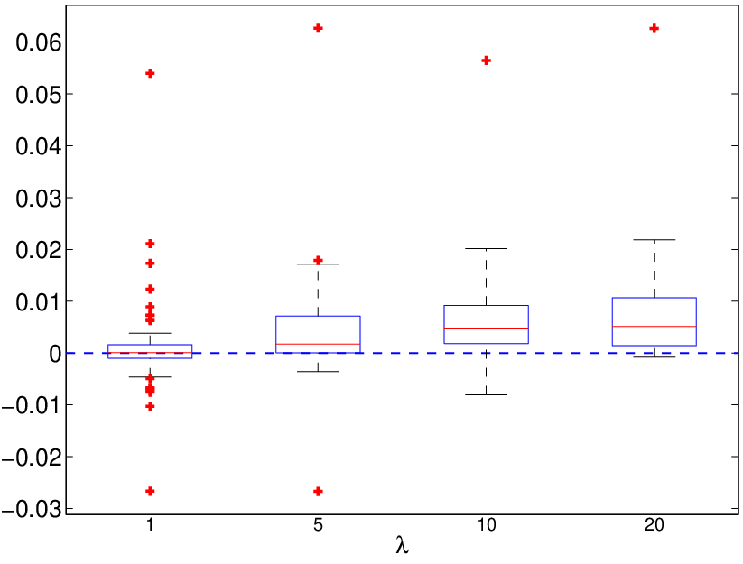
Similar conclusions were reached when using different values of $\alpha$ and $\beta$ and for the truncated Potts-DP model discussed in (11).

As we expect the number of clusters to be around ten, we evaluate the Potts-DP ¹¹ 1 Experiments were also performed with the two parameter Poisson-Dirichlet, but without observed improvement on the performances. and the truncated Potts-DP models with $\alpha=3$ and $\beta=0.02$ in agreement with Figure 2. We compare our results to mean-shift [3] and rdd-CRP [11]. We tested all these methods by randomly selecting 50 images from each of 8 categories in the LabelMe dataset (i.e. on a total of 400 images) and 200 images from the Berkeley dataset. We display the obtained results on six particular images in Figure 5. As expected the number of clusters decreases as $T_{\text{min}}$ increases.

To assess the quality of the image segmentation results, we use the rand index [15] computed using the “ground-truth” which is obtained through a manual labelling [24]. This comparison was also performed in [11] and the results are presented in Table 1. To evaluate the statistical significance of the results, we performed a Wilcoxon signed-rank test between the method with highest rand index (rdd-CRP for LabelMe and Mean-Shift for Berkeley dataset) and the other methods. We found no statistically significant difference (at the 1% level) between the performances of rdd-CRP, Potts-DP and truncated Potts-DP on the LabelMe dataset, and no statistical difference between Mean-Shift and Potts-DP on the Berkeley dataset.

Despite the significant differences observed visually when increasing the truncation threshold, e.g. see Figure 5, this does not translate in any improvement from the rand index point of view. However the manual labelling appears fairly subjective, so the rand index and the associated results have to be interpreted carefully.

References

- [1] A. Barbu and S.C. Zhu. Generalizing Swendsen-Wang to sampling arbitrary posterior probabilities. IEEE Transactions on Pattern Analysis and Machine Intelligence, 27(8):1239–1253, 2005.
- [2] A. Barbu and S.C. Zhu. Generalizing Swendsen-Wang for image analysis. Journal of Computational and Graphical Statistics, 16(4):877–900, 2007.
- [3] D. Comaniciu and P. Meer. Mean shift: A robust approach toward feature space analysis. IEEE Transactions on Pattern Analysis and Machine Intelligence, 24(5):603–619, 2002.
- [4] David B Dahl. Sequentially-allocated merge-split sampler for conjugate and nonconjugate Dirichlet process mixture models. Journal of Computational and Graphical Statistics, 11, 2005.
- [5] L. Du, L. Ren, D. Dunson, and L. Carin. A Bayesian model for simultaneous image clustering, annotation and object segmentation. In Advances in Neural Information Processing Systems, 2009.
- [6] J.A. Duan, M. Guindani, and A.E. Gelfand. Generalized spatial Dirichlet process models. Biometrika, 94(4):809–825, 2007.
- [7] R. E. Edwards and A. D. Sokal. Generalization of the Fortuin-Kasteleyn-Swendsen-Wang representation and Monte Carlo algorithm. Physical review D, 38(6):2009–2012, 1988.
- [8] C.M. Fortuin and P.W. Kasteleyn. On the random-cluster model:: I. introduction and relation to other models. Physica, 57(4):536–564, 1972.
- [9] S. Geman and D. Geman. Stochastic relaxation, Gibbs distributions, and the Bayesian restoration of images. IEEE Transactions on Pattern Analysis and Machine Intelligence, (6):721–741, 1984.
- [10] S. Ghosh and E.B. Sudderth. Nonparametric learning for layered segmentation of natural images. In Computer Vision and Pattern Recognition (CVPR), 2012 IEEE Conference on, pages 2272–2279. IEEE, 2012.
- [11] S. Ghosh, A.B. Ungureanu, E.B. Sudderth, and D.M. Blei. Spatial distance dependent chinese restaurant processes for image segmentation. In Advances in Neural Information Processing Systems, 2011.
- [12] P.J. Green. Reversible jump Markov chain Monte Carlo computation and Bayesian model determination. Biometrika, 82:711–732, 1995.
- [13] P.J. Green and S. Richardson. Hidden Markov models and disease mapping. Journal of the American Statistical Association, 97:1055–1070, 2002.
- [14] D.M. Higdon. Auxiliary variable methods for markov chain monte carlo with applications. Journal of the American Statistical Association, pages 585–595, 1998.
- [15] L. Hubert and P. Arabie. Comparing partitions. Journal of classification, 2(1):193–218, 1985.
- [16] Michael Hughes, Emily Fox, and Erik Sudderth. Effective split-merge monte carlo methods for nonparametric models of sequential data. In Advances in Neural Information Processing Systems, pages 1304–1312, 2012.
- [17] S. Jain and R. Neal. A split-merge markov chain monte carlo procedure for the dirichlet process mixture model. Journal of Computational and Graphical Statistics, 13(1), 2004.
- [18] J. Lau and P.J. Green. Bayesian model based clustering procedures. Journal of Computational and Graphical Statistics, 16:526–558, 2007.
- [19] D. Martin, C. Fowlkes, D. Tal, and J. Malik. A database of human segmented natural images and its application to evaluating segmentation algorithms and measuring ecological statistics. In Proc. 8th Int’l Conf. Computer Vision, volume 2, pages 416–423, July 2001.
- [20] Greg Mori, Xiaofeng Ren, Alexei A Efros, and Jitendra Malik. Recovering human body configurations: Combining segmentation and recognition. In Computer Vision and Pattern Recognition, 2004. CVPR 2004. Proceedings of the 2004 IEEE Computer Society Conference on, volume 2, pages II–326. IEEE, 2004.
- [21] P. Orbanz and J. M. Buhmann. Nonparametric Bayesian image segmentation. International Journal of Computer Vision, 77:25–45, 2008.
- [22] J. Pitman. Exchangeable and partially exchangeable random partitions. Probability theory and related fields, 102:145–158, 1995.
- [23] X. Ren and J. Malik. Learning a classification model for segmentation. In IEEE International Conference on Computer Vision, 2003, 2003.
- [24] B.C. Russell, A. Torralba, K.P. Murphy, and W.T. Freeman. Labelme: a database and web-based tool for image annotation. International journal of computer vision, 77(1):157–173, 2008.
- [25] E.B. Sudderth and M.I. Jordan. Shared segmentation of natural scenes using dependent Pitman-Yor processes. In Advances in Neural Information Processing Systems, volume 21, pages 1585–1592, 2009.
- [26] R.H. Swendsen and J.-S. Wang. Nonuniversal critical dynamics in Monte Carlo simulations. Physical Review Letters, 58:86–88, 1987.
- [27] G. Winkler. Image analysis, random fields and Markov chain Monte Carlo methods: a mathematical introduction, volume 27. Springer Verlag, 2003.