Active Information Acquisition
Abstract
We propose a general framework for sequential and dynamic acquisition of useful information in order to solve a particular task. While our goal could in principle be tackled by general reinforcement learning, our particular setting is constrained enough to allow more efficient algorithms. In this paper, we work under the Learning to Search framework and show how to formulate the goal of finding a dynamic information acquisition policy in that framework. We apply our formulation on two tasks, sentiment analysis and image recognition, and show that the learned policies exhibit good statistical performance. As an emergent byproduct, the learned policies show a tendency to focus on the most prominent parts of each instance and give harder instances more attention without explicitly being trained to do so.
Keywords:
reinforcement learning, learning to search, sequential prediction1 Introduction
In the supervised learning framework, a learning algorithm is given example input-output pairs with which to model the desired behaviour. However real life autonomous agents must dynamically acquire the information they need for decisions based upon goals and current knowledge. Thus the information required varies across different instances of the problem. Furthermore, given a time or expense budget, an algorithm can attempt to balance a trade-off between cost of acquiring information (and reasoning about it) and quality of the result. These considerations apply both to understanding psychophysical phenomena such as planning saccades (Araujo et al., 2001) and to developing practical solutions to problems such as early classification of time series (Dachraoui et al., 2015).
We propose a general-purpose framework that sequentially processes the input, adaptively selects parts of it, and combines the acquired information to make predictions. Our framework can be applied to any base model (e.g. generalized linear models, neural networks) with any information unit (e.g. features, feature groups or pieces of raw input).
Specifically, given a prediction task, our goal is to learn a task predictor and an information selector. The task predictor takes information acquired by the selector and generates outputs defined by the specific task, such as object classes for image classification. The information selector acquires pieces of information based on past information and intermediate predictions given by the task predictor. We model this dynamism as a sequential decision-making process as shown in Figure 1, where we make a decision about which information to acquire at each step. The process stops when the model decides that enough information has been obtained and outputs its final prediction. We use the Learning to Search (L2S) (Daumé III et al., 2014) framework, which casts searching for a good policy as an imitation learning problem: at training time we have access to (can simulate) a reference policy which is possibly accessing the training labels, and the goal is to induce a policy that mimics the reference policy at test time.
Our contribution is an active information acquisition model that is flexible enough to apply to different tasks with different predictors and information units. Our model explicitly minimizes a user-specified trade-off between cost on information and quality of prediction. We quantify the trade-off as the loss function for L2S. As there are no constraints on the loss function, our model can accommodate different types of loss defined by a task and even loss functions that do not decompose nicely over the search space.11 1 In some applications, the cost of a piece of information may depend on whether another piece of information has been acquired or not. The L2S framework additionally requires the specification of a search space, and a reference policy. Our formulation for these ingredients in the case of active information acquisition is detailed in Section 4.
We evaluate our algorithm on a sentiment analysis task with a bag-of-words predictor, and an image classification task with a convolutional neural network (CNN). Our algorithm achieves better results than static information selection baselines on both tasks. Additionally, we show that the dynamic selector learns to acquire more information for difficult examples than easy examples.
| Algorithm 1 Predict () 1: for to do 2: Intermediate prediction 3: Select information 4: if stop then 5: return Early stop, return terminal state 6: else 7: Add new information 8: end if 9: end for |
2 Related Work
The topic of learning information gathering policies has received much interest lately. Many of the proposals in this space however use general Markov decision process (MDP) techniques, which are sufficient but perhaps not necessary given the constrained, deterministic world of sequential selection.
Kanani & McCallum (2012) learn a policy for filling in missing entries in a knowledge base, where the actions are querying a search engine, downloading a page or extracting information from a page. For learning the policy, they use temporal difference Q-learning and briefly mention potentially more efficient techniques but always within the general MDP learning framework.
Our work is closest to Dulac-Arnold et al. (2011); Dulac-Arnold et al. (2014), who explored sequential text and image classification with results analogous to our experiments. The authors proposed reinforcement learning techniques with adaptation to different tasks, while our approach is general and efficient enough to apply to a range of problems. More importantly, when the complete inputs are available (but hidden to the learning algorithm), we can compute a good reference policy and incorporate it into L2S through imitation learning for more efficient training. Another important distinction is that they use a single policy as both the task predictor and information selector. This formulation has a larger search space compared to ours and does not leverage pre-training of the task predictor. In addition, it might face difficulty in complex domains where the predictor and the selector need different function classes.
Mnih et al. (2014) explored sequential visual inspection for image classification, with results analogous to our image classification experiment. Important technical differences are the use of policy playouts and the specific use of recurrent neural networks. Our approach admits the use of recurrent neural networks for either the predictor or selector components, but does not require it. In other words, the model is a special case of our framework with particular choices for the predictor and selector components. Furthermore, that work demonstrated improved aggregate performance with diminishing returns for fixed budgets of sensor utilization, but do not consider policies which make a variable number of sensory measurements. Similar comments apply to the recent visual attention work of Ba et al. (2015).
Our loss function quantifies the information-accuracy trade-off. Any approach leveraging general reinforcement learning can optimize such a loss: nonetheless, the prior art above did not do so. This trade-off can be critical in practical applications, e.g., minimum cost spam filtering (Blanzieri & Bryl, 2008), and has been treated explicitly in the case of classifier cascades (Chen et al., 2012) and early classification of time series (Dachraoui et al., 2015).
Our work is also related to dynamic feature selection. He et al. (2012) used DAgger (Ross et al., 2011) to select features sequentially with a loss function similar to ours. DAgger is a specific implementation of L2S that does not consider cost of errors, and we observe degrading results with uniform cost in our experiments. In addition, they consider information selection on the feature level only. In Gao & Koller (2011), classifiers are selected dynamically based on their value of information under a probabilistic framework. Again, they consider a particular form of information—observation presented as classification results—while we embrace a broader class of information.
Póczos et al. (2009) consider the problem of learning a stopping policy to maximize expected reward per unit time given a fixed sequence of classification strategies with variable associated temporal costs. A key distinction from this work is that the sequence of classification strategies is fixed, rather than trained jointly with the stopping policy.
3 Active Information Acquisition Framework
We assume that the input data can be decomposed to multiple parts, such that , where is the number of parts. We denote a partial input by , where . It is straightforward to extend the framework to input data with variable number of parts per example but we do not for ease of exposition.
Our framework consists of a task predictor and an information selector , which interact as shown in Figure 1. Both and access the input through feature maps, which we omit here to simplify notation.
The task predictor transforms a partial input into a prediction , e.g., for a multiclass problem the task predictor can take a partial input and produce a distribution over the labels.
The information selector is a policy that takes as input a state, which summarizes the information collected so far and any previous prediction(s), and outputs an action to take next: . The actions are (a) to acquire a new piece of information (and to specify which one) and (b) to stop and output the current prediction. The complete set of actions is . Added information is excluded from the action set, and we use to denote the action set specific to , including non-selected information and stop.
Our framework allows task-dependent choices of the learning components and . However, because these components must be able to work with any subset of input parts, idiosyncratic changes are required for different choices of . Handling missing and incomplete data is an area with an extensive literature. For our experiments, we find the following simple strategy effective: augmenting the input with an additional binary variable per part indicating whether or not a part has been observed and setting the feature values for the unobserved parts to 0.
4 Learning to Search for Information
Our framework builds on top of the Learning to Search (Daumé III et al., 2014) (L2S) paradigm, which allows us to jointly train the (interdependent) information selector and the task predictor via a reduction to online cost-sensitive classification.
The L2S algorithm requires three components: a search space which defines states, actions, and transitions, a loss function to evaluate the result given an action sequence, and a reference policy that suggests good actions given any state during training. Essentially, L2S learns a policy that imitates the reference policy, assuming that the reference policy attains good performance. Below we describe details of each component in our setting and the training algorithm.
Search space
Our state is a tuple of a partial input and an intermediate prediction: . The action set for is , which is defined in Section 3. We do not ask for the same piece of information more than once by disallowing actions corresponding to observed parts. This restriction is not necessary in other scenarios, such as a robot learning to act in a dynamic environment where the same part of the world may change over time. An illustration of the search space is shown in Figure 2. After an action is taken, the current state transitions to a new one deterministically by adding the new information or terminating the process, as shown in Algorithm 1, line 4–8.
Loss function
To learn a trade-off between the amount of information and the quality of the prediction, we define the loss function as
| (1) |
Here is the loss function defined by the task, which does not have to be convex, e.g., 0-1 loss, squared loss. is the cost function of information. In our experiments, we set , which computes the percentage of parts acquired. However, an arbitrary function of can be used for acquisition cost, e.g., for variable feature cost (Chen et al., 2012) or nonuniform cost of delay (Dachraoui et al., 2015). We use to control the penalty on acquiring more information. By varying we can construct a Pareto curve of cost vs. loss.
Since we compute intermediate predictions, the loss function can be applied to results at any time step. We call the loss at the end the terminal loss and those at earlier time steps the immediate loss, and our goal is to learn policies that minimize the expected terminal loss.
Reference policy
We use a greedy reference policy that always chooses the next piece of information that yields the lowest immediate loss. Formally,
where . As the performance of L2S depends much on the quality of the reference policy, we analyze in Section 5 when a greedy policy is optimal and how suboptimality affects the result. We have also verified that this policy is performing well on the tasks in Section 6, in fact leading the learned policy by a large margin. Unlike our learned policy however, the reference policy makes use of the training label and therefore cannot be used at test time.
Joint Training
During training, L2S calls the Predict function (Algorithm 1) many times to explore different action sequences and to discover the ones that have a low terminal loss, similar to other reinforcement learning techniques. However, with a reference policy, L2S can explore the search space more efficiently by initially focusing on areas close to the action sequences generated by the reference policy and gradually deviating away by following the learned policy (Daumé III et al., 2014).
We show the training procedure in Algorithm 2. For each example, we collect a set of cost-sensitive multiclass examples, where class labels correspond to actions. First an initial trajectory is generated (roll in) by the current learned policy ,22 2 We can also roll in with a mixture of the reference policy and the learned policy and gradually decrease the mixing weight of the reference policy. We did not observe significant difference by using a mixture roll-in policy. then from the arrived state, the reference policy is executed until the terminal state (roll out) to derive the terminal loss of each action. The cost assigned to an action in a given state is the difference between its loss and the minimum loss for the state (Algorithm 2, line 10). Rolling in with the learned policy guarantees that states of the collected examples are representative of states encountered at test time. Given tuples of state, action and loss as training examples, the policy learning problem is reduced to standard cost-sensitive multiclass classification.
We assume that an initial task predictor is given and intermediate predictions are generated by calling it. To initialize a task predictor beforehand, we pre-train one on a small portion of the training data, e.g., by using randomly sampled subsets of parts. This pre-training distribution is presumably unlike the one induced by a mature selector. To mitigate this, we fine-tune the task predictor during training with inputs generated by the information selector after each update (line 13–16 in Algorithm 2).33 3 In practice, fine-tuning may happen after some iterations when the selector is relatively stable. In other words, we adjust the task predictor to reduce the loss of each intermediate prediction on the partial input sequences generated by the selector .
5 Analysis
We now analyze the quality of the information selector returned by Algorithm 2. As L2S minimizes loss relative to the reference policy, we measure performance of the learned policy by regret to . We first present the regret guarantee of L2S, then extend the result to our setting of information selection.
The loss of a policy is defined as the expected terminal loss, and the expectation is taking over distribution of the states induced by running . We use to represent the terminal loss of executing action in state and then following policy until the terminal state. We denote by the distribution of states at step when running policy and , where is the horizon length, namely the maximum number of parts of the input. Thus we have
Henceforth, we use as a shorthand for .
L2S has the following regret guarantee:
Theorem 1.
When using a no-regret cost-sensitive learner, the policy returned by Algorithm 2 after steps satisfies
where is defined as
In words, the regret is bounded by the expected difference in cost-to-go of the reference policy induced by a suboptimal action, and increases linearly with the sequence length. Readers are referred to Chang et al. (2015) for the proof.
Now we specify the bound in our setting. First we define suboptimality of a reference policy. Starting from any state, if the optimal policy achieves terminal loss , a reference policy with suboptimality achieves a loss no larger than ().
Notice that the Q-values in differ only when a classification error occurs. We denote the classification error of a policy as , such that with probability , chooses the same action as .
As we are bounding the error of a general framework without making specific assumptions about the task predictor and the cost function, we assume bounds on the following variables; however, we discuss the range of these values at the end of this section. Given any information set, we denote by the maximum difference in task loss due to changing one piece of information (a insertion, deletion or substitution). Further, we let be the maximum cost-to-go from any state of the reference policy, and be the maximum acquisition cost of one piece of information.
With the above definitions, we have the following guarantee for active information selection:
Corollary 1.
If the returned policy has error rate when evaluated in the multiclass classification setting, as an information selector it satisfies
where .
Proof.
Let be the final information set obtained by executing in and then following . Now consider an auxiliary policy whose actions only depend on : it copies the action given by at the same time step after regardless of its own state. Let , . The trajectories of and diverge from time when . Therefore starting from , the final information sets obtained by and differ by one element only due to . We use to denote the information set obtained by copying , which replaces information acquired by with that by in . Therefore we have .
Now we can write the -function as the loss in the terminal state. To simplify notation, we use as a shorthand for ; and similarly, for . For the th example we have
| (2) | |||||
The inequality is due to the definition of suboptimality of . Further, we have 44 4 We omit in when obvious from the context.
The first inequality is from Equation 2. In the last step, the difference between task loss due to one-step deviation is bounded by by definition; similarly, their costs differ by one element only which is at maximum. To concisely present our result, below we denote the RHS (a constant) of the above inequality by .
Discussion
In practice, is often close to 1. For example, if is a matroid defined on , meaning that each part contributes to the loss independently, then the greedy reference policy is optimal and . If is a monotone, submodular, non-negative function, the greedy reference policy has suboptimality bounded by . In the simple case where the cost function measures the cardinality of a information set, we have . The maximum cost-to-go is small when the state is on the trajectory of ; otherwise it depends on the how well can recover from a bad state. In cases where adding information monotonically improves the result—as we will see in the experiments— can recover fast by selecting useful information even if some less distinctive ones were added.
Therefore, the performance of our algorithm is mainly affected by two factors. The first is the classification error of . Given enough examples (), this is solely restricted by the policy class and the feature representation of states, suggesting a richer policy class may work better. The second is the robustness of the task predictor to slight change in received information, affecting . This can be addressed by pre-training on randomly sampled subsets and by fine-tuning with partial inputs induced by the learned policy .
6 Experiments
We evaluate our algorithm AIA on two tasks with different information sets and task classifiers: sentiment analysis and object recognition. We show that AIA consistently performs better than the static selection baseline. Furthermore, it achieves a good trade-off between cost and accuracy by acquiring more on hard examples than on easy examples.
All of our implementation is based on Vowpal Wabbit (Langford, 2007),55 5 http://hunch.net/~vw, a fast learning system that supports online learning and L2S. Unless stated otherwise, we run L2S for 2 passes over the training data; fine-tuning the predictor starts at the end of the first pass.
6.1 TL;DR: Sentiment Analysis of Book Reviews
In this experiment the task is to predict a user’s rating by reading their reviews sentence by sentence from the beginning. We use sentences as the units of information. The model dynamically decides whether to continue reading the next sentence or to stop and output the current predicted rating, hence we refer to it as TL;DR (“Too Long; Didn’t Read”).
We evaluate TL;DR on book reviews from the Amazon product data (McAuley et al., 2015), where each review has an associated rating between 1 and 5 inclusive. We select reviews with 5 to 10 sentences and split the dataset into three sets: 1M for pre-training the task predictor, 8M for L2S and fine-tuning and 1M for testing. Our task predictor is a linear multiclass classifier using unigrams and bigrams features of tokenized text. We pre-train the predictor on complete reviews and all prefixes.
Our information selector is a quadratic multiclass classifier. The features are the intermediate scores (negative log likelihood) for each class as given by the task predictor; the difference between the highest and the next-highest score, i.e. the score margin; the KL-divergence between the current scores and the class prior66 6 The prior class distribution is imbalanced in this dataset: more than 50% reviews have a rating of 5.; the current prediction of the task predictor, i.e., the argmax of the scores; and the number of sentences read so far.
We sweep over to obtain a range of models that reads different numbers of sentences on average. Larger discourages the model to use more information. We compare performance of our dynamic model with a baseline static model given various fixed amounts of information. Our baseline model always selects the first sentences (), and utilizes a task predictor trained on the first sentences using all the examples L2S uses as training data (i.e., both the pre-training and fine-tuning data sets). We report macro-F1 versus the average percentage of sentences read in Figure 3 and our model completely dominates the static selection method.
To examine where the model decides to acquire more information, we compute the average percentage of sentences for each rating. We took four models with different s and plot the result in Figure 3 (right). As increases, the model reads fewer sentences on average since the penalty on cost becomes higher. In addition, the model reads much fewer sentences for the easy rating-5 (a majority class in our dataset) reviews and more for confusing reviews in the middle. This shows that the model learns to acquire information adaptively according to example difficulty.
6.2 TB;DL: Image Recognition
In this experiment the goal is to recognize objects by looking at a few patches from an image. This scenario is a toy version of a robot/camera trying to making sense of a scene by deciding where to focus. Our model starts from an empty image and adaptively selects a sequence of patches to examine until it feels confident about the prediction and stops. We refer to the model as TB;DL (“Too Big; Didn’t Look”).
We evaluate our algorithm on an image classification task from PASCAL VOC Challenge 2007. We resize all images to . Each image is divided into 25 equal-sized square patches, where each patch is a part. Our task predictor takes features extracted from the selected patches and predicts the objects in the image. There are 21 object classes including the background. For simplicity, we focus on the task of predicting whether a person is in the image (the majority class that often co-occurs with other classes). To obtain patch features, we label each patch with its image (multi-)label and fine-tune the pre-trained VGG-16 (Simonyan & Zisserman, 2014) model from Caffe with the patch examples. We use the predicted probabilities output by the softmax layer of VGG network as the patch features.77 7 We have also tried to use features from the penultimate fully-connected layer but found it was not helpful. The state features are based on intermediate scores, similar to TL;DR.
We compare against static selectors that always select a fixed subset of patches. As it is computationally expensive to enumerate all possible subsets, we heuristically selected a family of subsets that cover the image from the center to the outer parts, as shown in Figure 4 (right). We obtain similar results to the sentiment analysis task: active information acquisition shows a better trade-off than static selection. In fact, the static baseline eventually shows degradation when shown larger portions of the image. We speculate this is because VOC images often contain multiple, scattered objects with background clutter. Under such conditions, a limited static focus might be better than a larger one, but a dynamic focus is best. This supposition is supported by our heat map experiment.
|
|
|
|
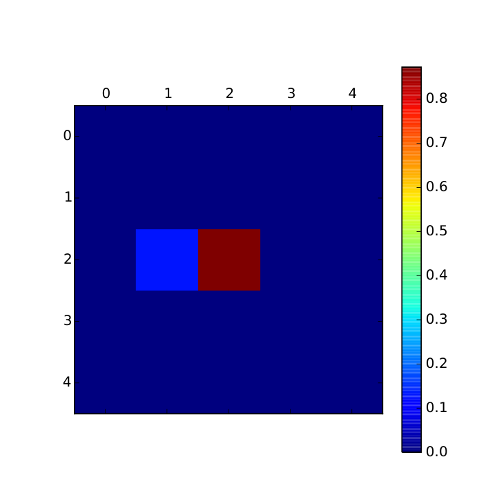
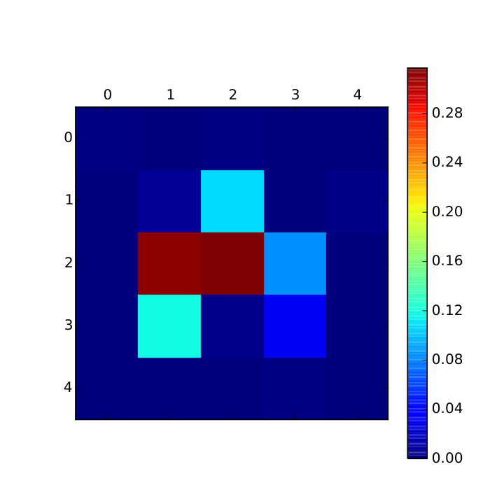
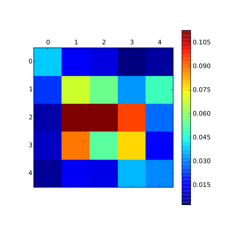
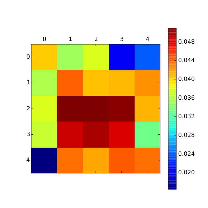
To examine where the model pays most attention, we show heat maps of the attention of models with different trade-offs in Figure 5 (best viewed in color). The result is consistent with our intuition: when the amount of information is restricted, the learned policy looks mostly in the center where the object is more likely to be located; when more information is allowed, the policy dynamically explores outer parts. Furthermore, when information acquisition is free, i.e., when , the model still chooses to classify before viewing the entire image, indicating a limited static focus can be beneficial even absent acquisition costs.
The VOC dataset also contains annotations about hard instances, which we use to confirm that the model learns to use more information for hard examples. In Figure 6, we report the average number of patches selected for both hard and easy examples. When is large, the policy selects approximately the same number of patches for both types of images, since the cost penalty does not allow for more exploration. When the constraint on cost is relaxed, we see that for difficult images the average number of patches selected is consistently larger than that for common images.
7 Conclusion
In this paper we showed how to formulate the task of learning to acquire information for solving a particular problem inside the L2S paradigm. We proposed a computationally simple reference policy (that has access to the training labels) and used imitation learning to compete with it, avoiding the difficulties of more general reinforcement learning techniques. We also proposed a loss function that explicitly balances the trade-off between the task loss and the cost of information acquisition. The effect of minimizing this trade-off is the learned policies focus on the prominent parts of the input and spend more effort on examples that are harder to classify.
We believe that much of the existing work on dynamic information gathering can leverage imitation learning and the L2S framework instead of falling back to more general reinforcement learning techniques. For example, in early classification of time series, the future is eventually observed, which facilitates constructing a reference policy at training time. Therefore, fruitful directions for future work include adapting and extending the ideas we presented in this paper to other domains where the active collection of information can be simulated at training time.
References
- Araujo et al. (2001) Araujo, Christian, Kowler, Eileen, and Pavel, Misha. Eye movements during visual search: The costs of choosing the optimal path. Vision research, 41(25):3613–3625, 2001.
- Ba et al. (2015) Ba, Jimmy, Salakhutdinov, Ruslan R, Grosse, Roger B, and Frey, Brendan J. Learning wake-sleep recurrent attention models. In Advances in Neural Information Processing Systems, pp. 2575–2583, 2015.
- Blanzieri & Bryl (2008) Blanzieri, Enrico and Bryl, Anton. A survey of learning-based techniques of email spam filtering. Artificial Intelligence Review, 29(1):63–92, 2008.
- Chang et al. (2015) Chang, Kai-Wei, Krishnamurthy, Akshay, Agarwal, Alekh, Daumé III, Hal, and Langford, John. Learning to search better than your teacher. In Proceedings of the International Conference on Machine Learning (ICML), 2015. URL http://hal3.name/docs/#daume15lols.
- Chen et al. (2012) Chen, Minmin, Xu, Zhixiang (Eddie), Weinberger, Kilian Q., Chapelle, Olivier, and Kedem, Dor. Classifier cascade for minimizing feature evaluation cost. In Proceedings of the Fifteenth International Conference on Artificial Intelligence and Statistics, pp. 218–226. MIT Press, 2012.
- Dachraoui et al. (2015) Dachraoui, Asma, Bondu, Alexis, and Cornuéjols, Antoine. Early classification of time series as a non myopic sequential decision making problem. In Machine Learning and Knowledge Discovery in Databases, pp. 433–447. Springer, 2015.
- Daumé III et al. (2014) Daumé III, Hal, Langford, John, and Ross, Stéphane. Efficient programmable learning to search. In arXiv, 2014. URL http://hal3.name/docs/#daume14lts.
- Dulac-Arnold et al. (2011) Dulac-Arnold, Gabriel, Denoyer, Ludovic, and Gallinari, Patrick. Text classification: a sequential reading approach. In Advances in Information Retrieval, pp. 411–423. Springer, 2011.
- Dulac-Arnold et al. (2014) Dulac-Arnold, Gabriel, Denoyer, Ludovic, Thome, Nicolas, Cord, Matthieu, and Gallinari, Patrick. Sequentially generated instance-dependent image representations for classification. In Proceedings of ICLR, 2014.
- Gao & Koller (2011) Gao, Tianshi and Koller, Daphne. Active classification based on value of classifier. In Proceedings of NIPS, 2011.
- He et al. (2012) He, He, Daumé III, Hal, and Eisner, Jason. Imitation learning by coaching. In Proceedings of NIPS, 2012.
- Kanani & McCallum (2012) Kanani, Pallika H and McCallum, Andrew K. Selecting actions for resource-bounded information extraction using reinforcement learning. In Proceedings of the fifth ACM international conference on Web search and data mining, pp. 253–262. ACM, 2012.
- Langford (2007) Langford, John. Vowpal Wabbit. https://github.com/JohnLangford/vowpal_wabbit/wiki, 2007.
- McAuley et al. (2015) McAuley, Julian, Targett, Christopher, Shi, Qinfeng, and van den Hengel, Anton. Image-based recommendations on styles and substitutes. In Proceedings of SIGIR, 2015.
- Mnih et al. (2014) Mnih, Volodymyr, Heess, Nicolas, Graves, Alex, et al. Recurrent models of visual attention. In Advances in Neural Information Processing Systems, pp. 2204–2212, 2014.
- Póczos et al. (2009) Póczos, Barnabás, Abbasi-Yadkori, Yasin, Szepesvári, Csaba, Greiner, Russell, and Sturtevant, Nathan. Learning when to stop thinking and do something! In Proceedings of the 26th Annual International Conference on Machine Learning, pp. 825–832. ACM, 2009.
- Ross et al. (2011) Ross, Stéphane, Gordon, Geoffrey J., and Bagnel, J. Andrew. A reduction of imitation learning and structured prediction to no-regret online learning. In Proceedings of AISTATS, 2011.
- Simonyan & Zisserman (2014) Simonyan, Karen and Zisserman, Andrew. Very deep convolutional networks for large-scale image recognition. In arXiv, 2014. URL http://arxiv.org/pdf/1409.1556.pdf.