Phase Structure of 1d Interacting Floquet Systems I: Abelian SPTs
Abstract
Recent work suggests that a sharp definition of ‘phase of matter’ can be given for some quantum systems out of equilibrium—first for many-body localized systems with time independent Hamiltonians and more recently for periodically driven or Floquet localized systems. In this work we propose a classification of the finite abelian symmetry protected phases of interacting Floquet localized systems in one dimension. We find that the different Floquet phases correspond to elements of , where is the undriven interacting classification, and is a set of (twisted) 1d representations corresponding to symmetry group . We will address symmetry broken phases in a subsequent paper.
I Introduction
The past few years have seen considerable progress in our understanding of the phenomenon of many body localization (MBL) which has built on the early[1], seminal and rigorous[2] work that established its existence. One of the more interesting ideas that has emerged from this work is that of eigenstate phase transitions wherein individual many body eigenstates and/or the eigenspectrum exhibit singular changes in their properties across a parameter boundary even as the standard statistical mechanical averages are perfectly smooth. In recent work [3] this idea was generalized to disordered Floquet systems taking advantage of the fact that they exhibit generalizations of the notions of eigenstate and eigenvalue in the form of time-periodic Floquet eigenstates and associated quasi-energies. Ref. 3 presented evidence that one dimensional spin chains with Ising symmetry exhibit four distinct Floquet phases with either paramagnetic or spin glass order – two of the resulting Floquet phases have no analogs in undriven systems. Disorder seems to be an essential ingredient in this generalization – if the driving Hamiltonians are clean[4, 5, 6, 7], or lack sufficiently strong disorder[8], the eigenstate properties of periodically driven systems seem to exhibit “infinite temperature” ergodic behavior, with no vestige of paramagnetic or spin glass quantum order.
In this paper we pick up the thread from this point and address the question of obtaining an enumeration of all possible Floquet phases in one dimension. Specifically, we restrict ourselves to Floquet phases which do not spontaneously break any symmetry of the drive; we will analyze the case of broken symmetry in a subsequent paper. In 1d this implies that we are looking for Floquet versions of symmetry protected topological (SPT) phases of matter, which generalize topological insulators and superconductors to interacting systems.
All SPT phases of matter are associated with some global symmetry group , which is not spontaneously broken. Given a symmetry group there may be many distinct SPT phases, each of which can be distinguished by their ground states – two ground states represent the same SPT phase iff they can be connected to one another by a symmetric local unitary. A complete classification of SPTs in 1d is available [9, 10]. The first step away from the purely ground state classification was taken in Refs. 11, 12 where it was shown that in the presence of localization induced by sufficiently strong disorder, the entire spectrum (not just the ground state) of certain SPTs can carry a signature of the underlying SPT order. In 1d this is the statement that in many-body localized SPT systems, the entire spectrum has a characteristic string order. This idea was clarified recently in Ref. 13. On the one hand MBL Hamiltonians are believed to be characterized by the appearance of a complete set of local integrals of the motion or bits [14, 15, 16]. On the other hand, it is known that a proper subset of the possible SPT orders can be captured by commuting stabilizer Hamiltonians11 1 A commuting stabilizer Hamiltonian takes form , where the are local and commute amongst themselves. See Ref. 12 for a well explained example of a commuting stabilizer SPT Hamiltonian, and examples in the main text.. Ref. 13 synthesized these observations arguing that only those SPT orders captured by commuting stabilizer Hamiltonians can have eigenstate order.
In another line of work, non-interacting Floquet systems have been investigated for non-trivial topology and building on various examples [18, 19, 20, 21, 22, 23, 24] a classification has recently been obtained [25, 26], and also investigated in a disordered setting[27, 28]. This classification is indeed richer than for the undriven problem. As Ref. 25 shows, if the original equilibrium non-interacting classification was [29], then the Floquet classification is of form .
Here we will show that the classification of symmetric Floquet states is different from both the undriven MBL SPT classification and the non-interacting Floquet classification; a simple example is given by the bosonic SPT considered in detail in Sec. V. Our general approach is as follows. We start with a Floquet drive with associated Floquet unitary . We assume that has a prescribed eigenstate order which we call the bulk order (measured by a string order parameter for unitary , and encoded in the form of the local conserved quantities). To focus on those Floquet systems potentially resilient against heating to “infinite temperature”, we consider only those bulk orders which are many-body localizable in the sense of Ref. 13 – in practice, this means we restrict ourselves to states with on-site symmetry groups . We make a further simplification by assuming is abelian.
In the undriven setting, the classification of 1d SPT eigenstate order is captured by how the symmetries in the problem act projectively at the edge[30, 9, 10], this being captured almost entirely22 2 For fermionic states, the fermion parity of the symmetry action at the edge is also important[30]. by a so-called 2-cocycle 33 3 See also Ref. 48, 10 for a more pedestrian exposition, and Ref. 49 and Sec. IV for an introduction to cocycles.. We conjecture that in the driven MBL setting in addition to this information there is just one further piece of data characterizing the commutation between the symmetry action local to the edges and the Floquet unitary itself. For unitary symmetries, we show that this is a 1d representation of . For anti-unitary symmetry groups of form where is unitary and is time reversal, our results are less certain, but we conjecture that obeys a twisted 1-cocycle condition Eq. (15). In any case, the set of all such is denoted . Hence our proposed interacting classification for Floquet drives is of the form where Cl is the undriven classification. A compatible set of results was obtained independently shortly after the appearance of the present work in Refs. 33, 34, 35.
To support our conjecture we investigate in more detail the structure of local symmetric Floquet unitaries with a complete set of local bulk integrals of motion. On an open chain, we argue that such a unitary can be brought into a form where are local to the left/right end of the system and both commute with , a local functional of the local bulk conserved quantities characterizing the bulk order. We formulate in terms of , and show that it is robust under arbitrarily large but symmetric modifications to the Floquet drive local to the edges as well as small symmetric perturbations to the bulk.
The balance of the paper is set out as follows. We start in Sec. II with a 1d Floquet system with class D (fermion parity protected) Kitaev chain eigenstate order. We use a novel framework to reproduce the classification obtained from band theory, and verified in an interacting setting in Ref. 3. This helps us to motivate a more general framework in Sec. III. Then in Sec. IV we reinterpret our results more simply as an extension of the undriven algebraic classification of Ref. 30. In Sec. V we examine the spectrum of the interacting bosonic drive, explaining what kinds of edge modes are present. In Sec. VI we deal separately with two examples of time reversal invariant SPTs, the latter being an interacting driven version of fermionic Class BDI. We conclude in Sec. VII.
II Motivating example: Class D in 1d
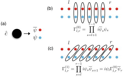
We will now consider in some detail a particular case that will explain the logic we follow in the general case. This is the case of Floquet drives defined by fermionic Hamiltonians which conserve fermion parity. For quadratic time independent Hamiltonians this is Class D in the Altland-Zirnbauer classification. We will use the same nomenclature for our interacting time dependent problem. For the non-interacting Floquet problem the list of phases for Class D is known and we will explain how this exhausts the list of phases in the interacting MBL setting as well; we note that previous work [3] has shown by explicit computation that the non-interacting phases do continue into this setting but not settled the question of whether others exist. We now, successively, review the basics of the time independent quadratic classification, its Floquet analog and an understanding of the latter appropriate to the MBL setting and end with the promised generalization to interacting MBL Floquet systems.
II.1 Time independent SPT phases
There are just two SPTs with just fermion parity symmetry in 1d[9, 30]. They have model Hamiltonians
where the Hilbert space consists of spinless fermion degrees of freedom , or equivalently two Majorana fermion degrees of freedom per site defined by . If we choose the to be translationally invariant then encode the well known Kitaev trivial/topological 1d wire fixed point states. Hamiltonians in the same phase as are called topological because they are associated with an (exponentially) protected spectral pairing on an open system associated with a protected Majorana mode at its edge. Concretely, for presented above, we can find simultaneous eigenstates of and fermion parity . The operator commutes with but anti-commutes with . Hence each energy eigenvalue of is associated with at least two states with fermion parity respectively. , the trivial state, has no such protected degeneracies.
Another way to distinguish the ground states of the trivial/topological phases is through the use of string order parameters. That is, if we define
| (1) |
then is long-ranged/exponentially decaying in the trivial/topological phases respectively, and is long-ranged/exponentially decaying in the topological/trivial phases respectively (see Ref. 36 for an illuminating account of string order in 1d SPTs). We will thus refer to the trivial/topological states as having type string orders respectively. If we choose strongly disordered all of the eigenstates of necessarily have string order of types respectively, and this statement is at least perturbatively stable to the inclusion of interactions[13].
II.2 Quadratic Floquet phases
There are four known phases of the Class D Floquet problem. Following Ref. 3 we can exhibit them in a simple model of a binary Floquet drive (see also Ref. 21) using the reference Hamiltonians
where we pick to be uniform. Eventually we will disorder these couplings, but we assume uniformity for now for ease of exposition. The final Floquet unitary is simply
| (2) |
The phase diagram of our binary drive as a function of has some manifest periodicities. Note that whence the replacement shifts all quasi-energies by but otherwise the Floquet eigenstate properties remain unchanged. The same holds true for shifts like . Hence the eigenstate properties of are invariant under . Another thing to note is that for systems with an even number of sites the unitary effectively flips while flips . Therefore the eigenstate properties of are also invariant under such inversions and reflections in . From this combination of shift and reflection symmetries in , it suffices to consider a unit cell of the phase diagram as shown in Fig. 2. The phase transition lines drawn in the diagram are straightforwardly obtained by diagonalizing for closed chains where each individual momentum sector only presents a two dimensional problem. Of these, the boundary at small , can be obtained by using the BCH formula to show that . In this regime, the eigenstates are determined by the effective Hamiltonian , which is expected to be fully trivial/topological for and respectively.
We will now develop an analytical, spatially local, picture of this phase diagram, which in turn will guide our attempt to classify 1d Floquet phases—we do this by focusing on the boundaries of the fundamental region where the Floquet unitaries will exhibit localization even absent disorder. In the regions labelled ‘triv’, representative unitaries are obtained by setting i.e., . It is clear that the eigenstate properties of these unitaries are simply those of the trivial Hamiltonian and all of the eigenstates have string order. This is clearly a consequence of the (trivial) localization of . In the region labelled ‘top’, representative unitaries are obtained by setting i.e., , so the eigenstate properties of these are simply those of the topological Hamiltonian . All of the eigenstates have string order and on an open system, this drive will have a protected Majorana at its edges commuting with , and a spectral pairing associated with this Majorana.
The topological phase is new to the driven setting. As an example, set and
This is simply the unitary associated with a topological drive (discussed above) multiplied by the global fermion parity operator which is itself a good quantum number of . There is a complete basis of eigenstates with topological string order, which follows from the fact they have local integrals of the motion of form . Now, rewrite in terms of said local integrals of the motion to obtain
This unitary looks like the topological drive above (with shifted), multiplied by a term which commutes with the bulk local integrals of motion. Thus we can diagonalize the bulk unitary and the edge unitary simultaneously, writing eigenvalues of as where are the eigenvalues of the bulk and edge unitaries respectively. Note that anti-commutes with and commutes with the bulk unitary. Hence if is an eigenvalue of then so is . In other words if then has eigenvalue . This shift symmetry in the argument of associated with the boundary Majoranas is the reason we call this state the topological state.
In summary, we identified the eigenstate order of the drive, wrote the unitary in terms of the corresponding local integrals of motion. The resulting unitary looked like a simple topological drive multiplied by a term which hops Majoranas between the distant edges. This implied a spectral pairing at quasi-energy .
We can treat the phase analogously. On the boundary of that region, the eigenstates have type (trivial) string order Eq. (1) and at a given edge, there is a and a quasi-energy Majorana mode. To see this, set and . The resulting unitary simplifies to
| (3) |
In the last line we used a local symmetric unitary change of basis (implemented by ). Note that the on-site fermion parities are local integrals of motion in the bulk (). As in the previous example, we use these local integrals of motion to re-express the unitary as
| (4) |
This looks like a bulk non-topological drive multiplied by a Majorana tunneling operator . Note that the edge degrees of freedom are completely decoupled from the bulk so we can simultaneously diagonalize the bulk unitary and the two site edge unitary
Note that the two boundary sites involve the four Majoranas . This two-site unitary has two useful independent integrals of motion and – note these are also integrals of motion of the original unitary as well. Picking a reference eigenstate of for the two site problem, we can toggle between the four eigenstates of as shown in Table 1.
Note that the edge degrees of freedom have two eigenstates at each of . It is straightforward to use the edge properties listed in Table 1 to show that the eigenstates of the full Floquet unitary come in quadruplets with eigenvalues . From Table 1 we see that is associated with a flip while is associated with . Hence we think of as being a zero/ quasi-energy Majoranas respectively.
Finally we can offer some intuition regarding the somewhat physically opaque constructions. The non-trivial drives (i.e., the and drives) are associated with a tunneling operator of the form . We can think of these operators as pumping fermion parity charge from one edge to the other, across the entire system. So non-trivial Floquet drives differs from trivial Floquet drives insofar as a charge of the symmetry group has been pumped across the system.
II.3 Generalizing to the MBL regime
We were able to understand the specific class D drives above by reducing the Floquet unitary to the form
| (5) |
where is some functional of local bulk l-bits , and are operators localized at the left and right edges of the system respectively which commute with all bulk . For the non-trivial Floquet drives (i.e., the and drives), were both fermion parity odd unitary operators.
This begs the question: Can we always reduce to this simple form, and does the fermion parity of always indicate whether or not the Floquet drive is trivial? We claim yes. In full, we will argue that fermion parity symmetric Floquet unitaries with a complete set of bulk local integrals of motion and an associated trivial/topological eigenstate order : (i) can be written as Eq. (5); (ii) have definite (and identical) fermion parity as operators, and (iii); the parity of is uniquely determined by and robust to arbitrarily large parity symmetric modifications to the unitary near the edges, and sufficiently small bulk perturbations.
For (i) it is essential to assume the existence of local conserved quantities – this is presumably necessary at the outset if we wish for our system to not heat up in the sense of Refs. 4, 5, 6, 7. In App. A we argue that can be chosen to be a local function of these local conserved quantities because arises from a time dependent local Hamiltonian. Before diving into the fuller discussion of the more general case in Sec. III, and assuming (i), let us give some flavor of the arguments for (ii),(iii). Using Eq. (5), and the fact that commutes with both and the bulk l-bits, it follows that where we define
for invertible operators . Now, as is a local unitary circuit (of depth 1), it is straightforward to see that is a unitary localized near the left/right end of the system respectively. Indeed we can write and where is some unitary operator localized near the left/right end of the system. implies
| (6) |
But are local to respectively, distant from one another, and yet inverse to one another. The only possibility is that is a pure phase. Using the fact that it moreover follows that . Thus, have definite and equal fermion parities.
For (iii) we need to show that the parities remain unchanged if we augment our drive where are parity symmetric unitaries localized near the left/right edges of the system respectively. Heuristically speaking, we are just modifying , which will not change the fermion parities of because are parity symmetric – of course, this is a little misleading, because the modified do not necessarily commute with all of the bulk l-bits as required in Eq. (5). A fuller argument is provided in Sec. III.3. See also App. C and App. D for a distinct and potentially tighter argument using string order parameters.
Last, we wish to argue that the parity of is robust to sufficiently small bulk perturbations. This statement is supported by the observation that in the non-interacting Floquet setting with a random disorder configuration, the and Majoranas eventually decay into the bulk with probability . The decay length is determined by the average behavior of the random couplings (see Ref. 37 for an example of such a calculation, using transfer matrices). Upon modifying the bulk couplings smoothly, the decay length changes smoothly, and for sufficiently small changes the Majorana edge mode is robust with probability . Thus in the non-interacting setting, the edge structure is at least statistically robust to small adjustments to the bulk. In our formalism when the are parity odd, they are the many body analogues of the Majoranas in the non-interacting setting. In this case we expect a similar statistical statement to hold. Namely, upon modifying the bulk couplings slightly, the operators remain fermion parity odd, and localized to the edges with probability .
III General Framework
The discussion in the previous sections focussed on a fermion parity symmetric system . Here we consider more general Floquet drives with an on-site finite global abelian symmetry group with global generators . Start with some spatially local -symmetric and time-periodic family of Hamiltonians , giving rise to an instantaneous unitary . Our aim is to characterize the eigenstates of on a system with edges.
We assume that has full eigenstate order i.e., assume that the disorder in the drive is sufficiently strong such that there is a complete set of local integrals of the motion (l-bits) , which encode a known unique SPT order. As discussed in the introduction, only certain SPT eigenstate orders are expected to exist stably as the eigenstate orders of Floquet unitaries. For this reason, we restrict our attention to such ‘many-body localizable’ SPT orders from the outset. In 1d Ref. 13 suggest all SPTs with finite on-site symmetry group are many-body localizable. It is for this reason we consider finite discrete , and for simplicity we focus on abelian .
We make a technical assumption about the l-bits: we assume they can be chosen to commute with the global symmetry generators. This latter requirement is certainly true for 1d fixed point MBL abelian SPT phases[13]. Perturbing symmetrically away from the fixed point models, we expect the l-bits to be smeared out , in such a way that also commutes with the global symmetries. While the l-bits at the fixed points are exactly local, the are only exponentially local[38].
The more general arguments in this section will follow the same format as before in the class D case. We argue that finite abelian symmetric Floquet unitaries with a complete set of bulk l-bits and an associated trivial/topological eigenstate order : (i) Can be written as Eq. (5) (with obeying the conditions stated below Eq. (5)); (ii) can be associated with a certain (twisted) 1d representation of to be defined; (iii) this 1d representation is uniquely determined by and robust to arbitrarily large symmetric modifications to the unitary near the edges, and sufficiently small bulk perturbations. (i)-(iii) together suggest that the symmetry protected features of Floquet drives with the mentioned properties are captured by the bulk order and the (twisted) 1d representation . Therefore, labelling the possible bulk orders by ClG and the possible (twisted) 1d representations by , we conjecture that the interacting Floquet classification is Cl for the considered here.
This section is organized as follows. We supply the arguments for (i) in App. B. In the next two sections we show (ii), i.e., how to associate with a certain 1d (twisted) representation of . This will involve demonstrating that the quantity
| (7) |
which we call the ‘pumped charge’, defines a (twisted) 1d representation of . Our discussion is split between the unitary and anti-unitary cases in Sec. III.1 and Sec. III.2 respectively. Eq. (7) involves a generalization of the group commutator defined by
| (8) |
where is any unitary, and is a homomorphism with for unitary/anti-unitary respectively. Note that for unitary , .
In Sec. III.3 we argue (iii), i.e., is well defined and robust to arbitrarily large symmetric adjustments to the unitary local to , and sufficiently small bulk perturbations. Finally in Sec. III.4 we summarize our proposed classification, and provide some examples.
III.1 Unitary on-site symmetry groups
Recall that is generated by a symmetric family of Hamiltonians . This implies that commutes with the global symmetry generators i.e., for all . We use this fact to constrain the symmetry properties of the appearing in Eq. (5).
Lemma 1.
Consider system , and finite abelian unitary symmetry group . Then are scalar operators, where is a global symmetry transformation.
Proof.
From assumption (i) we argued that the Floquet unitary takes form Eq. (5) where are localized at the edges, and commute with . The unitary is -symmetric so for all . In addition, commutes with the global symmetry generators because it is a function only of l-bits, which are all assumed to commute with the global symmetries. Therefore
| (9) |
The RHS of this equation can be expressed as (abbreviating to and to )
| (10) |
The second equality follows because and commute. To show this, it suffices to note (a) both terms are localized at the edges respectively, and (b) in a fermionic system at least one of these terms is fermion parity even. (a) follows from the fact is a low-depth unitary, so are local to the part of the system respectively. (b) follows from the earlier argument around Eq. (6) that have definite parity , so that has parity as required. Eq. (9) and Eq. (10) together imply that . But then are unitaries with support far away from one another, yet have . The only possibility is that are of the forms respectively. ∎
III.2 Time reversal () symmetry
We can apply most of the arguments in the above subsection to drives with symmetry group where is unitary and is time reversal, but there are a few complications. First in Lemma 1 we used the fact that . This follows for unitary symmetries because each of the instantaneous Hamiltonians are symmetric from which it readily follows that is symmetric. In contrast, if is time reversal symmetric then will not necessarily obey . However, if we insist in addition that [25] where is the period of the drive, then is guaranteed for all including .
The next stumbling point in attempting to formulate an analogue of Lemma 1 is in showing that
| (12) |
where is the bulk part of the unitary Eq. (5). While Eq. (12) is clear in the unitary case it is less clear in the non-unitary case, and in fact we will only prove it for a subset of the time reversal invariant SPTs. To see where the problem arises, express
where is a sum over all the possible values for all l-bits, and are necessarily U numbers. By assumption the global time reversal generator commutes with all the l-bits . Then Eq. (12) holds provided . One way to guarantee this is to consider only those SPT orders for which the eigenvalues are real e.g., . We will assume this condition, as it is automatically true in the cases we wish to consider in this text Sec. VI.
Assuming then that Eq. (12) is true, Eq. (9) must hold. We now revisit the argument in Lemma 1 to find (abbreviating to , to , and to )
| (13) |
The second equality follows from the fact that is fermion even and localized to the right hand edge as before. The third equality follows from the fact have definite and identical fermion parity as before. Hence, using Eq. (9) we find that . But, as have support far away from one another we must have
| (14) |
is a pure phase as before. It again follows readily that . One slight difference however is that
Therefore the analogue of pumped charge in this non-unitary case obeys
| (15) |
so that is a ‘twisted’ analogue of a 1d representation of the group .
III.3 Robustness of pumped charge
Having associated with (twisted) 1d representation , we now show (iii), namely that is: (a) well defined i.e., independent of the precise manner in which we decompose Eq. (5); (b) robust to symmetric modifications of the unitary at the edges; and (c) robust to sufficiently small symmetric bulk perturbations.
To show (a), suppose we have two decompositions obeying the conditions below Eq. (5). Are the pumped charges the same? We argue yes. First we restrict attention to those terms in involving only conserved quantities in some extensive connected sub-region of the bulk which is nevertheless far away from both , forming functional . From the locality of it follows that acts like the identity over almost all of . Indeed
| (16) |
where are functions of bulk l-bits on left/right parts of the system respectively which are widely separated from one another. Now commutes with by assumption, and commutes with because it is supported far away from . It follows readily from Eq. (16) that commutes with , a fact we will use shortly. Now, as act identically deep in the bulk it is also true that acts like the identity over most of , and it has a similar decomposition into unitaries based at the left and right sides of the system, and as before commutes with . Now multiplying by we obtain
As have support far away from , it follows that
where is some U phase, using the same reasoning deployed below Eq. (6) and in Lemma 1. Applying to this equation shows have the same pumped charge because bulk l-bits commute with the global symmetry generators, and commute with respectively. Thus we have argued that the pumped charge is well defined.
For (b) we need to show that the pumped charge is robust to local symmetric changes at the edge. Under such modifications, the resulting unitary will still have a complete set of conserved quantities deep the bulk so still has bulk eigenstate order. We just need to show that the pumped charge is robust under modifications of form for some symmetric localized near (say) the left edge such that continues to hold. Under such a modification will change, as will some of the l-bits near the left end of the chain. However for large system size, should not change under such a modification, and so neither does . Hence from the constraints Eq. (14) between , the pumped charge cannot change. For an alternative and perhaps more rigorous characterization of the pumped charge for systems with unitary symmetry group , which does not require the knowledge that we can decompose , see App. C. Unfortunately, in the anti-unitary case, some of the methods of App. C are inapplicable because of the well known[39] difficulties in defining a ‘local time reversal’ string operator.
Last we come to the slippery issue of whether the pumped charge is robust to sufficiently small bulk perturbations, and we give a similar argument as for the class D subclass in Sec. II.3. Our expectation is that for a random disorder configuration, are with probability localized to the edges with a localization length determined in part by the spatially averaged values of the local couplings comprising . Under sufficiently small changes to these local couplings, we therefore expect the localization length and to change smoothly. For truly small changes in and , the pumped charge being discrete (a twisted 1d representation) cannot change and remains fixed.
III.4 Summary and examples
Thus, for 1d Floquet drives with finite on-site abelian symmetry group and paramagnetic bulk order, our proposed Floquet classification looks like where is the undriven paramagnetic classification, and consists of all of the 1d (twisted) representations of group . Table 2 gives examples.
The undriven classification can be read off from existing results [30, 9]. For a unitary abelian , the 1D representations are in bijective correspondence with itself. So the Floquet classification takes the form for finite unitary abelian groups. For class D, we see that , so our scheme (which applies to interacting systems) reproduces the Floquet classification result seen in the non-interacting band theory context[25]. There are numerous examples of groups where , so that our prediction breaks the pattern seen in the non-interacting classification up until now[25]. For example, for one obtains and – see Sec. V for a description of the model, and examples of drives.
On the other hand, for symmetry groups with time reversal of the form where is finite on-site unitary, we show in App. F that the possible twisted 1d representations are precisely i.e., specified by a d unitary representation of and a choice of . For abelian this implies a Floquet classification of form . For example, for we get Floquet classification . On the other hand for a ‘BDI’ fermion system with we obtain Floquet classification – although, see Sec. VI.2.1 where we argue that in certain regards the classification can be regarded as . The free fermion Floquet classification of the BDI system gives , so we observe an interaction induced breaking of results similar to that seen in the non-driven context Ref. 30. We direct the reader to Sec. VI for a further discussion of this point, and examples of the different drives. As an aside we note that Note that, while our formalism includes the possibility of anti-unitary symmetries, the notion of eigenstate order and MBL in these scenarios has not yet been established in detail (see discussion in Ref. 13). For this reason our results with non-unitary groups should be considered with caution.
| On site Symm. (G) | Undriven classif. (ClG) | Twisted 1d reps. () | Floq. MBL PM classif. () |
|---|---|---|---|
IV An algebraic characterization
Having argued that the pumped charge is a robust property of symmetric Floquet unitaries with eigenstate order, we now show how the presence of the pumped charge affect the spectra of Floquet unitaries. In the process we condense our results into a concise algebraic formalism. We do this by extending the formalism of Ref. 30, which was developed to deal with equilibrium SPT states. In this undriven setting, Ref. 30 starts by considering the nearly degenerated ground states of an SPT on an open 1d chain . These ground states are indistinguishable in the bulk, and differ only near . The global symmetry group acts on the this low energy space. By locality, for an extensively large system, the global symmetry must act like within this space, where localized near the end of the system respectively. Note that are only defined up to phases, and indeed need only obey where is a -cocycle defining a projective representation of (similar for the right edge). To consider anti-unitary symmetry groups, it is helpful to define a homomorphism where for unitary/anti-unitary respectively. With this in mind the associativity of the action on say the left edge leads to a relation
| (17) |
which is the defining relation for a 2-cocycle. Ref. 30 then argue that this 2-cocycle is the relevant datum identifying the SPT in question. Within the low energy subspace, in the thermodynamic limit, must act like a scalar, and it can be argued that individually commute with the Hamiltonian. Hence, the low energy subspace is some representation of the algebra generated by the operators . The form of this algebra is determined entirely by the choice of cocycle 44 4 As well as the fermion parity of the in fermionic systems.. This is the classification of D SPTs in brief. For system’s whose entire spectrum is MBL with SPT eigenstate order, the above statements hold not only for the ground state subspace, but for a complete set of degenerate multiplets of excited eigenstates.
Consider now a Floquet SPT drive on an open chain with full eigenstate order. We can play a similar game. Again we can fix the bulk eigenstate (i.e., bulk conserved quantities) and consider the symmetry action in this restricted subspace. Again, when we consider the symmetry acting on a particular edge, we find that it is characterized by some 2-cocyle . However, in the Floquet case there is potentially another datum determining the edge structure. In particular, while previously commuted individually with the Hamiltonian, in the Floquet case we see that need not necessarily commute with . To see this, let us treat unitary and anti-unitary separately.
In the previous section we saw that the Floquet unitary takes the form . Fixing the bulk state – i.e., the conserved quantities in the bulk – the Floquet unitary acts like . We argued in Lemma 1 that the global symmetry commutes with individually up to a phase characterized by . This quantity, in turn, determines the commutation between and . So, the algebra of symmetry operators in the edge space are characterized by a 2-cocycle and , which defines a 1d representation of the gauge group. For fermionic systems one should bear in mind the possibility that operators on distant edges may anti-commute if they are fermion parity odd.
Recall that in the anti-unitary symmetry group case we call the Floquet unitary symmetric if can be chosen to be a symmetric Hamiltonian. This means that . As before, consider the action of into the edge subspace, which again by locality takes form . The global symmetry in this case should obey (see Eq. (8)) – although we were unable to prove this in the anti-unitary case. Assuming we can, we have – this information is captured by just one quantity . This quantity in turn determines the commutation relations with the edge symmetry operators . So the symmetry algebra at the edge is again characterized by a 2-cocycle and a U phase . When the symmetry group is anti-unitary, this phase does not quite form a 1d representation as in the unitary case. Instead it obeys Eq. (15) hence the data determining the drive are where is a kind of twisted 1d representation, the set of which we denote .
Having proposed a classification for 1d Floquet SPT drives, in the next two sections we describe some instructive examples. First in Sec. V we look at an interacting bosonic Floquet SPT drive with . Then in Sec. VI we look at two examples of drives with anti-unitary symmetry groups of form – the latter is of particular interest, as it corresponds to an interacting version of the fermionic BDI symmetry class. In all cases, we will provide explicit examples of drives within each of the proposed Floquet phases.
V Edge structure for Floquet drives
In this section we focus on bosonic paramagnets with unbroken global symmetry. This example is interesting because it involves an intrinsically interacting bosonic system, and it breaks the ClCl classification pattern seen in the classification of non-interacting fermionic Floquet drives[25]. To wit, has an undriven SPT classification of Cl, corresponding to a trivial paramagnet and non-trivial SPT state, while we predict in Sec. III a classification. After describing the SPT order in the undriven setting, we provided examples of drives in each of the eight putative phases in the conjectured classification. We describe the edge theory for some of these drives using the formalism of Sec. IV.
Consider a chain with on-site local Hilbert space where . Let be the operators measuring , and let act as and respectively. It is clear that behave like Pauli-matrices. States with global symmetry generators have a classification from group cohomology – hence there are two SPT fixed points, corresponding to the trivial paramagnet and SPT
| (18) | ||||
| (19) |
respectively. Both model Hamiltonians are sums of commuting operators. The l-bits for the trivial paramagnet are while those for the SPT are . As alluded to in Sec. IV, we can fix the ‘bulk’ conserved l-bits appearing in Eq. (19), and ask how the global symmetry transformations act on the residual edge degrees of freedom – the forms of the generators projected onto this subspace with fixed l-bits is summarized in Table 3.
| Generators\Bulk order | triv. pm | spt | ||
|---|---|---|---|---|
| L | R | L | R | |
V.1 MBL Binary drives realizing the Floquet phases
Here we construct examples of drives for the eight putative Floquet phases. We use a three part drive of the form
| (20) |
where is one of , while are chosen from
In , we choose disordered with mean . In all of the eight examples, we always set or . For these choices of , we can use the identity to show that
where (for instance) looks like one of
The two possible choices of (trivial PM or SPT), along with the four choices of above, give the eight elements of the classification . By construction, the drive in question has a complete set of exactly local bulk conserved quantities (from ), and with some minor local symmetric changes of basis at the edge (similar to those below Eq. (3)) can be chosen to commute with . Hence, the drive constructed gives a ‘fixed point’ realization of the different Floquet classes predicted by our framework in Sec. III. In the remainder of the section, we examine a selection of the eight constructed drives, and explain the structure of their eigenspectra. A detailed discussion of the edge states for all eight cases can be found in App. E.
V.1.1 Undriven example:
In these cases the unitary is just
so the spectrum of is just the spectrum of . Fixing the bulk l-bits we know that the symmetry action factorizes as , and the exponentially degenerate eigenspaces form representations of the algebra generated by .
For trivial paramagnetic for instance, the states need only form a representation of the algebra generated by . As all of the elements of this algebra commute, representations of this algebra can be 1 dimensional. In physical terms there are no protected degeneracies at the edge of this system[30].
On the other hand, for , furnish a projective representation of the symmetry group – those listed in Table 3. Fixing the bulk integrals of motion, the residual edge degrees of freedom form some representation of the algebra generated by for all . In the present case the symmetry generators at a particular edge do not generally commute. This non-commutation of the symmetry generators implies that there is at least a protected a two-fold degeneracy associated with each edge – indeed, in the present example, there is exactly a two-fold degeneracy associated with each edge. So the spectrum of the Floquet unitary has a spectral pairing, with every eigenstate being a part of a pair at the same quasi-energy.
V.1.2 Non-trivial Floquet example
In this example we set and respectively, and . The resulting Floquet unitary is of the form
Using a local symmetric change of basis we can rewrite this as
with and , which commute with the bulk l-bits for . Fixing the bulk l-bits, the Floquet unitary acts like
on the edge degrees of freedom. Looking at the commutation relations between the global symmetry generators and gives pumped charge . As the bulk order is trivial paramagnetic, the symmetry operators at the edge look like from Table 3. Having fixed all the bulk l-bits, the remaining edge degrees of freedom form a representation of an algebra
As a result, we can show that the possible edge states come in quadruplets (two protected degrees of freedom at each edge). These quadruplets do not all lie at the same quasi-energy as was the case in the undriven case, but the quasi-energy spacings are protected. To see this, first note that has a centre generated by . As these operators commute with all of their eigenvalues can be fixed. This amounts to modding out the centre and considering the representations of the algebra .
To establish the representations of it is helpful to (following Ref. 41) identify a maximal commuting sub-algebra . We proceed by picking a simultaneous eigenvector of the generators of – denote the corresponding eigenvalues respectively. Consider acting on this state with the remaining elements of the algebra. We get at least four states with different eigenvalues in . Table 4 shows the distinct states arising from this procedure. We also record the eigenvalues of which simply act like in this eigenspace. In summary, fixing the bulk l-bits, we find there are four edge states (two at each edge) spread evenly between two eigenvalues . Within each eigenspace, there are two eigenstates distinguished by the eigenvalue, for instance.
| Params.\Class. | ||||||||
| - | - | |||||||
| - | - | - | - | - | - |
VI Anti-unitary examples
| Drive\ | ||||
| - | - |
| Drive\ | ||||
| - | ||||
| - | - | |||
| - | - | - | ||
In this section we grapple with SPT drives with time reversal symmetry. As such SPTs are not as well understood in the context of MBL and eigenstate order[13] our results in this section are more tentative, and based on the heuristic arguments in Sec. III.2 and Sec. IV. In this section, we will deal with two examples of SPTs with abelian symmetry groups with time reversal, namely . We check that the arguments of Sec. III.2 certainly apply to these two cases, so that the classifications are of form respectively as predicted, and give examples of drives which should fall into each putative Floquet phase. We highlight in particular the case, which is a Fermionic system with time reversal symmetry (called ‘BDI’ in the free fermion context). Our results show that the free fermion classification of the BDI Floquet classes breaks down from (see Refs. 25, 26) to in the presence of interaction in a manner similar to that seen in the undriven setting[30].
VI.1 , bosonic system
First consider a bulk SPT phase with just symmetry and . We have not found an explicit discussion of such phases in the literature, although the relevant cohomology calculation is found in Ref. 9. First construct the undriven SPT states. Consider a system with an Ising degree of freedom on each site, and a symmetry where is complex conjugation. An example of such a Hamiltonian
| (21) |
has paramagnetic order and no symmetry protected edge state. On the other hand
| (22) |
has edge states which transform according to a projective representation 55 5 Note that a clean variant of Eq. (22) emerges in the high frequency expansion of the interacting drives considered in Ref. 50.. Note that are commuting stabilizer Hamiltonians, and the local integrals of motion commute with while taking values , so that the arguments of Sec. III.2 apply. According to that discussion, and to the discussion in Sec. IV, there will be just two possible Floquet phases for a given bulk order, distinguished by the pumped charges . This pumped charge in turn determines the commutation relations between and the Floquet unitary restricted to the edge subspace .
Here we claim to construct examples of the four Floquet pumps using trinary drives. It is useful to define an auxiliary ferromagnetic drive
| (23) |
Consider Floquet pumps of the form
| (24) |
All we need to do is specify and are either Eq. (21) or Eq. (22), where we choose to be say log-normal distributed with mean . The possible classes of drives will be labelled by where determine the SPT cocycle and hence the bulk order, while as discussed above. Table 6 summarizes which Hamiltonians need to be chosen for a given Floquet phase .
VI.2 Interacting BDI drives i.e.,
Here we put forward a tentative classification of interacting 1d ‘Class BDI’ MBL Floquet drives. The symmetry group is where time reversal obeys on the fundamental fermions. The undriven problem has a classification[30]. From Sec. IV, we expect the Floquet drives to have a classification, in contrast to the classification found in the non-interaction band theory picture [25, 37]. We now attempt to explain this collapse in classification using some example drives. First in Sec. VI.2.1 we consider stacking a number of the (clean) class D drives considered in Sec. II. Then in Sec. VI.2.2 we use another realization of the same SPT order and Floquet phase involving a single Majorana chain coupled to additional Ising degrees of freedom.
VI.2.1 Stacking argument
In this section we get a more concrete feel for how the part of the Floquet classification comes about by stacking many class D time reversal symmetric drives. While the stacked models we consider will have many extraneous bulk degrees of freedom, it allows us to extract useful intuition. Consider a drive with Kitaev Majorana chains, and with net Floquet unitary
| (25) |
label chains and
Note that the local conserved quantities in each of these Hamiltonians take values in and commute with time reversal symmetry as per the requirements of Sec. III.2. The Majoranas are such that and .
To obtain a drive with zero quasi-energy Majoranas and quasi-energy Majoranas at (say) the left edge, set and set , and and where say (the specific value is unimportant). The resulting Floquet unitary is
Note that so that are Majoranas and are zero Majoranas.
Consider a drive with bulk classification . By the eightfold Kitaev-Fidkowski classification, we may as well choose the above drive with any – it is convenient for our purposes to choose so that there are at least chains present. We will find that the properties of as a function of Majoranas comprising , namely , depend only on modulo .
First note that if , . Note this term can be removed from by extending the old Floquet drive by a local term
| (26) |
The resulting drive is still time reversal invariant, and in particular . The modification also respects local parity symmetric. The same thing can be done at the right hand edge. Hence, we have locally and symmetrically modified the Floquet drive to obtain
This Floquet unitary can clearly be engineered using a time independent Hamiltonian drive with bulk eigenstate order, on a system with boundary. Hence, when it comes to robust eigenstate properties, the drive should be considered the same as the drive with the same bulk order. Using this style of argument, it readily follows that the robust physical properties of a drive of form Eq. (25) with any should depend only on .
Let us now show that have distinct physical properties. Note first that cannot be removed in the above manner. This follows from . If we modify using some unitary acting on the left edge Majoranas, then the new Floquet unitary must have the time reversal property
| (27) |
where the last equality follows from the fact that has the same time reversal property as , namely . Were it possible to completely remove with such a , then . But this is inconsistent with Eq. (27).
The drives with are clearly non-trivial (from the class D part of the paper) because is fermion parity odd. What remains however, is to show that is distinct from . In fact this follows readily using the above method: Note that while . The different time reversal properties of these potential mean they cannot be locally tuned to one another while preserving time reversal invariance. In summary, fixing bulk class , there appear to be four distinct drives labelled by the four combinations of numbers . Thus the different Floquet drives appear to be labelled by elements of . Note that as sets (though not as groups) is equivalent to , so we could also say that the Floquet phases lie in the set . This latter presentation is preferable if one wishes the classification group to reflect the fourfold (see Eq. (26)) manner in which the pumped charge changes as we stack multiple Floquet systems atop one another. In other words one can view different Floquet phases as forming an abelian group , with addition corresponding to taking a tensor product of systems.
VI.2.2 Alternative setup
Consider a chain with and onsite Hilbert space consisting of majoranas, as well as a degree of freedom where a Pauli-matrix. Let time reversal act like where is complex conjugation. Then the Majorana fermions have the usual time reversal transformations, and . It can be verified (although we have not found an appropriate reference) that the following Hamiltonians capture the eight possible MBL phases of Fidkowski and Kitaev[30] with symmetry
These are all commuting stabilizer Hamiltonians, each l-bit taking values , and the stabilizers commute with both fermion parity symmetry and time reversal, so they obey the conditions discussed in Sec. III.2. To get any of the worth of Floquet phases it pays to consider three auxiliary Hamiltonians
and drives of the form
| (30) |
To obtain a drive first pick , the Hamiltonian with bulk order ‘’. For such a fixed choice of , the various choices of for the four possible are summarized in Table 7, as are the corresponding forms of the . In the language of Sec. III.2, the four possible correspond to the four possible twisted representations, with . As before, for all the Hamiltonians involved in the above drives, we will ensure is say log-normal distributed with mean . All of the drives so constructed are ‘fixed-point’ in the sense that they have a complete set of exactly local integrals of the motion in the bulk.
VII Concluding remarks
We have put forward a classification scheme for many-body localized Floquet SPT states in one spatial dimension with finite unitary on-site symmetries. In our scheme Floquet drives are classified by where ClG is the non-driven SPT classification, and is a set of 1d representations of (i.e., . We have also tentatively extended these methods to cases with time reversal for which where is unitary. In these cases the classification is again of form , but . In addition, we have given examples of idealized drives which realize the predicted putative Floquet phases.
The current work can be extended in several directions. There is the possibility of investigating driven analogues of disordered anyon chains[43]. In a sequel to this work [44], we use a similar toolkit to classify the possible symmetry broken Floquet phases in 1d; due to localization such order can indeed be observed in apparent violation of the standard theorems on broken symmetry and dimensionality. The extension of these results to higher dimensions is a fit subject for study, especially given recent questions over the existence of MBL phases in . Also left to future work is the detailed connection between the edge-based classification used in this paper and the bulk diagnostics used in Ref. 3. Finally there is the challenge of understanding the dynamical stability of these new phases for realistic drives en route to proposals for realizing and detecting them in experiments.
Note: Three closely related independent works appeared shortly after we posted this manuscript[33, 34, 35]. The first two of these references phrase the classification in terms of the second cohomology where is the global on-site symmetry group and is to be identified with time translation by one Floquet period. This interpretation is similar to that in our discussion in Sec. IV – indeed, the operators can be thought of as time translations local to the edges respectively. With this interpretation in mind, Sec. IV establishes how time-translation acts together with the other symmetries at the edge of the system. This is in fact the same thing as calculating the projective representations of the total symmetry group – that is, calculating .
Acknowledgements.
We thank V. Khemani, R. Moessner and A. Lazarides for many discussions and for collaboration (with SLS) on prior work. We would also like to thank R. Roy for generously sharing his unpublished work on the topological classification of free fermion drives. We thank A. Potter for alerting us to his work[34]. CVK is supported by the Princeton Center for Theoretical Science. SLS would like to acknowledge support from the NSF-DMR via Grant No. 1311781 and the Alexander von Humboldt Foundation for support during a stay at MPI-PKS where this work was begun.Appendix A Locality of
Consider a Floquet unitary on a system without boundary, with a complete set of local integrals of motion. Then may be written as a function of these local conserved quantities . We now give a sketch of an argument that may be chosen to be a local function of these conserved quantities. We use the fact that is a priori the result of a local unitary evolution. Local unitary evolutions may be well approximated by finite depth quantum circuits[45] – for simplicity let us assume that is a binary quantum circuit of depth (e.g., Fig. 3), where remains finite in the thermodynamic limit.
As a warmup, we argue that for local conserved quantities separated in excess of distance , and well in excess of the size of the local conserved quantities , the Floquet unitary can be written as where depends on but not , and depends on but not .
Consider a set of local conserved quantities associated with site . These quantities commute with one another, so we can find a simultaneous eigenbasis for the local Hilbert space. Label the distinct possible lists of simultaneous eigenvalues by integers . There may be degeneracies, so the eigenvectors corresponding to are of form . Let be a unitary which permutes all of the eigenvectors according to some permutation cycle . As permutes eigenvectors, it may also permute local eigenvalues through an action we denote .
is a local operator because it only permutes some eigenvectors in the local Hilbert space. As is local to and is low depth, the commutator is local to (this is a Lieb-Robinson type bound – except in the quantum circuit formalism there is no exponentially decaying tail). If was exponentially localized before, then the commutator is safely localized around certainly when considering distances much larger than and at least ! We call this the ‘smearing’ length scale .
If , then operators localized around should commute with i.e.,
| (31) |
where is any permutation. Consider components of this equation in the eigenbasis of local conserved quantities. depends on all the local conserved quantities in general, but we concentrate on the dependence of those conserved quantities near , writing where , and suppressing the other labels for now. The equation Eq. (31) reads
Pick such that and , and rearrange to find
| (32) |
The first factor on the right hand side depends on but not while the second depends on but not as required.
To argue that can be chosen to be local, concentrate on the factor . Now this implicitly depends on the values of other conserved quantities. Using the same reasoning as above and our previous result Eq. (32), we can factorize out the dependence of any for , namely (again suppressing dependence on other conserved quantities)
where the first term does not depend on , while the last two terms do not depend on . We can proceed inductively to show that
where are those labels at sites further than from , other labels are kept implicit, depends on and only conserved quantities within of , while does not depend on . In particular, is a local unitary which does not depend on . Moreover, one can verify for any site that is localized to within the same length scale of – with some thought, this follows from the fact that has smearing scale , and that is a product of factors with different combinations of conserved quantities set to . With this new site , repeat the procedure above (but using instead of ) to get
where depends only on conserved quantities near to , and is a local unitary which does not depend on and which also has smearing scale bounded by . Once can repeat this process inductively, cycling through all sites until eventually we find
where is a U function of conserved quantities within of , so can be written where is a real function of conserved quantities within of . As all the conserved quantities commute we have
up to a global U phase. We see that so defined here is at most a ‘-local’ Hamiltonian where . The argument above is clearly non-rigorous. We require a more careful analysis of the importance of exponentially small corrections in the iterative procedure outlined above.
Appendix B Form of
In this section, we first provide supporting arguments for (i) in the main text in Sec. B.1 – our arguments will rely heavily on the results of App. A. Then in Sec. B.2 we consider starting with a Floquet drive on a closed system, and show that upon restricting the Floquet drive to a subsystem, the resulting unitary also takes the canonical form Eq. (5).
B.1 Floquet MBL unitaries on systems with boundary
The main goal of this section is to support the claim (i) in the main text, that Floquet unitaries with a complete bulk MBL order, can be put into the form Eq. (5). We assume that is a local unitary on a system , with a complete set of l-bits in the bulk. Deep in the bulk, we know that is depends only on the bulk l-bits. Moreover using the results of App. A
where is a local functional of the bulk l-bits, and is some unitary acting near the boundary of the system. However, as is a local unitary circuit, and are very distant from one another, it follows that must factorize as
where are local to the left/right part of the system respectively. Consider a region where is much larger than the support of as well as the typical size of the conserved quantities. We can write
| (33) |
where are all those terms in which involve only conserved quantities in . While by locality involve only conserved quantities on the LHS/RHS of the system respectively (up to the exponentially small corrections mentioned in App. A). Note that all three terms on the RHS of Eq. (33) commute with one another because they only involve the conserved quantities. Note too that commute with because as operators they have disjoint support (and always fermion parity even). From the discussion of above, will commute with therefore
where commute with , and indeed all conserved quantities with support in the ‘bulk’ , as required. Having provided arguments supporting (i), we now give a method for deciding whether or not a Floquet drive defined on a system without boundary is in a trivial or non-trivial class.
B.2 Characterizing Floquet MBL unitaries on systems without boundary
We start with a definition.
Definition 1.
Given a many-body unitary evolution with a family of local bounded Hamiltonians on a closed system, we define the restricted unitary where are those terms in the Hamiltonian acting exclusively on subsystem .
We will show that if one takes a unitary circuit with full bulk MBL order on a manifold without boundary, and restrict to a system with boundary, the resulting unitary , can be put into the desired form Eq. (5). We will make use of the arguments in the previous section which showed that on a closed system, where is a local functional of bulk conserved quantities. First, a useful technical lemma.
Lemma 2.
Consider a local unitary circuit of depth . If on a closed system, then restricting to subsystem we find where are unitaries localized within of .
Proof.
Consider those circuit elements in the future Cauchy development of (the blue region in Fig. 3). Denote the unitary formed by multiplying out these circuit elements by 66 6 In the continuous time language, this is approximately the same as where , the notation denotes those terms in the Hamiltonian involving only sites in region , and is the Lieb-Robinson velocity.. Denote the rest of the unitary circuit by (red and purple in Fig. 3) . Then , and notably . However has support in while has support on a different set, namely the complement of . The only possible resolution is that both and have support only in the intersection of these two sets, namely . By Def. 1 we have where is formed of those circuit elements with support on but not in (purple circuit elements in Fig. 3). Thus has spatial support in within of or . The same statement is true of and hence also true for . Hence where has support in and has support in .
∎
Lemma 3.
A local Floquet unitary with eigenstate order restricted to subsystem takes form where are unitaries localized near the boundary, and .
Proof.
As has eigenstate order, and is low-depth, we assume we can write it as a local functional of local conserved quantities . Let be an extensive subregion of the system. The unitary circuit formed by concatenating and a circuit corresponding to . Now the unitary circuit , and is local by construction. Hence by Lemma 2 it has the property . On the other hand, from Def. 1 we have , where is just restricted to those terms involving only conserved quantities in . Hence we find . At this stage it is not clear that commute with . To make this clear, consider a region where is much larger than the depth of the circuit, and the size of the conserved quantities. We can write
where involves only conserved quantities on the LHS of the system, while involves those on the right and all three terms on the RHS commute with one another because they only involve the conserved quantities. Note too that commute with because as operators they have disjoint support (and always fermion parity even). From the discussion of above, continue to commute with if we redefine and , in which case
where commute with as required.
∎
Appendix C Alternative characterization of pumped charge for unitary symmetry groups
Here we give a slightly different definition of pumped charge which does not require the assumption that we can decompose . In the following we merely assume that is a local unitary with exact eigenstate order, and that the SPT order is many-body localizable and characterized by a string order parameter.
Definition 2.
A string order operator is a unitary function of of form where are unitary operators localized (with some correlation length ) near respectively, and is the on-site unitary symmetry operator.
Definition 3.
We say unitary has (exact) eigenstate order if it has a complete set of local conserved quantities taking the form with , and arbitrary sites in the system. Equivalently, where is a functional of a complete subset of all the local conserved quantities.
Definition 4.
Given subsystem we define special string order operator where is some point extensively far in the bulk (e.g., half-way along ). Similarly .
Lemma 4.
commutes with all local conserved quantities entirely in .
Proof.
is defined by writing down a conserved quantity on the original uncut system where is many to the left of , and restricting this unitary to . Indeed where is completely outside of . On the original uncut system, will a priori commute with all the conserved quantities in . Note then that . As the complement of is many correlation lengths away from (and necessarily fermion parity even), we must have . Hence . ∎
Lemma 5.
commutes with up to a phase. Moreover, using (A), this phase is equal to the older definition of pumped charge if we assume
Proof.
is supported almost entirely on some interval . Pick a point in this interval but many from . Then to good approximation where commutes with and local to . As a result . It follows from the fact is low depth and symmetric that is some operator with support near . Therefore for any but many away from the end-points. As the LHS does not depend on this implies is a pure phase. Now as commutes with all of the conserved quantities well in the bulk we have where unless both are fermion parity odd in which case . Now from the form of the string operator we know that where is the same as above because have the same fermion parity. Hence . ∎
Lemma 6.
The pumped charge defined above is robust under where are local (compared to the system size) symmetric unitaries which act only near the end of the system respectively.
Proof.
This follows from the previous lemma. On sites in the support of , acts like . But is symmetric (and assumed parity even in a system with fermions 77 7 In fermionic SPTs, fermion parity is always a symmetry, so as are symmetric they must also be fermion parity even[51].). Hence commutes with . Therefore remains unchanged. ∎
Lemma 7.
Time independent Hamiltonian (TIH) drives have trivial pumped charge.
Proof.
For a time independent Hamiltonian drive where is a symmetric local Hamiltonian. This Hamiltonian is assumed to have an eigenstate order . It follows that from the existence of such a string order that . As a result has the same eigenstate order, and . Hence . ∎
Appendix D Edge structure for Class D
In this section we use a different method to show how the Floquet phases in Sec. II arise. Suppose we are given a fermion parity symmetric, local unitary Floquet circuit on a large closed system. Suppose further that the Floquet unitary has eigenstate order – that is to say, there is a complete set of conserved quantites of the (approximate) form
where corresponds to trivial/topological eigenstate order respectively. On a system with boundary, we can arrange things so that
| (34) |
are a complete set of operators. The notation is explained in App. C. Our goal is to find the dimension and eigenvalues of a minimal representation of this algebra. Formally, we are looking for where is the center of the algebra. But in the present case, due to the bulk eigenstate order, contains all the bulk string operators, so we are indeed concerned only with where
| (35) |
The commutation relations of this algebra are
| (36) |
where and . One now asks what are the minimal dimension representations of this algebra? The answer is where .
D.1 Class D edges
Here we work out the representation theory of . The commutation relations for this algebra are
:
In this cases, all the generators of commute. Therefore is trivial, and there are no protected degeneracies in the Floquet spectrum. Therefore is trivial, and there are no protected degeneracies in the Floquet spectrum.
:
In this cases, none of the generators of commute. To elucidate the edge structure, we find a maximal commuting sub-algebra of . It is a convenient to choose because the eigenvalues of are up to a phase (from the bulk) just the eigenvalues of . Starting with a simultaneous eigenstate for , we get a minimal representation of size summarized here:
:
In this case , so the remaining sub-algebra is . To elucidate the edge structure, we find a maximal commuting sub-algebra of . It is a convenient to choose . Starting with a simultaneous eigenstate for , we get a minimal representation of size .
:
In this case , so the remaining sub-algebra is . A maximal commuting sub-algebra is . Starting with a simultaneous eigenstate for , we again get a minimal representation of size .
D.2 MBL Binary drives realizing the Floquet phases
The four possible Floquet phases here described can be realized using binary drives, as demonstrated in [3]. A binary drive involving Hamiltonians and times is a unitary matrix function of time
In the context of class D, we set
Setting , we can get the full classification by using which correspond respectively to obtain .
Appendix E Representation theory of edge in general, using string order method
Continuing from Sec. V, let us discuss the string order in PM and SPT states. The different forms of l-bits lead to a different kinds of string order in the two resulting SPT phases. Multiplying the l-bits together, notice that the eigenstates of the paramagnet can be chosen to be eigenstates of the string operators
| (37) |
The two operators can be though of as local generators of the symmetry, corresponding to group elements respectively. On the other hand, the eigenstates of the SPT can be chosen to be eigenstates of
| (38) |
These operators (away from ) also look like symmetry generators. Now move away from from the fixed point and consider a disordered scenario with the same symmetry group, and a complete set of l-bits. Away from the fixed points, we still expect there to be string operators which commute with the Hamiltonian, which are unitary functions of of form where are unitary operators localized (with some characteristic length scale ) near respectively, and is the on-site unitary symmetry operator – corresponding to for respectively. We will say that the Hamiltonian is in the trivial MBL PM phase if it commutes with a family of string operators which at large distances take a form approaching Eq. (37) while it is said to be in the SPT phase if they take the form Eq. (38). With these string operators in mind, we remind the reader how to define an action of the symmetry group at each edge (see App. C).
Definition 5.
Given subsystem we define modify the above string order operators to form where is some point extensively far in the bulk (e.g., half-way along ). Similarly .
In the MBL phase, these operators act like symmetry generators at each edge, and can be argued to commute with the bulk conserved quantities (see Lemma 4). For this reason, it is natural to identify them with from the previous section.
E.1 Edge structure
Now suppose we are given a unitary with prescribed bulk eigenstate order ‘’ and corresponding string order operators . By Lemma 5, commutes with up to phases characterized by a 1d representation . The set of operators which commute with up to phases are simply
| (39) |
Our goal is to find the dimension and eigenvalues of a minimal representation of this algebra. Formally, we are looking for . Due to the bulk eigenstate order, is simply generated by the bulk string operators. Hence, we are interested only in the algebra
| (40) |
The commutation relations of this algebra are
| (41) |
where and . This suggests a Floquet classification . Here if we take (reverting to additive notation). One now asks what are the minimal dimension representations of this algebra? The answer is if either or .
Now we work out the representation theory of . The commutation relations for this algebra are
:
In this cases, all the generators of commute. Therefore is trivial, and there are no protected degeneracies in the Floquet spectrum. Indeed is trivial.
:
For a non-trivial character of , there is a unique such that . Let another independent generator by . With this information, we can show that . Forming , we examine maximal commuting sub-algebra generated by representatives . See Table 8.
:
For a non-trivial character of , there is again a unique such that , and again denote another independent generator by . With this information, we can show that there is no nontrivial center. We examine a maximal commuting sub-algebra generated by representatives . The result is a minimal representation of size . See Table 9.
Appendix F Twisted 1d representations
Given a symmetry group of the form where is the time reversal symmetry group with , and is some unitary symmetry group, we wish to find all obeying
| (42) |
with . In particular, note that so that . Note that for any
Hence, restricted to , is just some 1d representation of . Hence, each solution determines an element and an . These two data determine entirely: For general with the defining relation Eq. (42) gives
| (43) |
Let us now ensure that for any choice of there is a corresponding solving Eq. (42). Define through Eq. (43). For any we have
Hence, the distinct solutions to Eq. (42) correspond bijectively with the 1d representations of , and a certain index (. Hence, we say there is a classification.
References
- [1] D. M. Basko, I. L. Aleiner, and B. L. Altshuler, Annals of Physics 321, 1126 (2006).
- [2] J. Z. Imbrie, arXiv:1403.7837 [cond-mat, physics:math-ph] (2014), arXiv: 1403.7837.
- [3] V. Khemani, A. Lazarides, R. Moessner, and S. L. Sondhi, arXiv preprint arXiv:1508.03344 (2015).
- [4] A. Lazarides, A. Das, and R. Moessner, Phys. Rev. E 90, 012110 (2014).
- [5] L. D’Alessio and M. Rigol, Phys. Rev. X 4, 041048 (2014).
- [6] D. Abanin, W. De Roeck, and F. Huveneers, arXiv preprint arXiv:1412.4752 (2014).
- [7] P. Ponte, Z. Papić, F. Huveneers, and D. A. Abanin, Phys. Rev. Lett. 114, 140401 (2015).
- [8] A. Lazarides, A. Das, and R. Moessner, Phys. Rev. Lett. 115, 030402 (2015).
- [9] X. Chen, Z.-C. Gu, and X.-G. Wen, Phys. Rev. B 84, 235128 (2011).
- [10] A. M. Turner, F. Pollmann, and E. Berg, Phys. Rev. B 83, 075102 (2011).
- [11] A. Chandran, V. Khemani, C. R. Laumann, and S. L. Sondhi, Phys. Rev. B 89, 144201 (2014).
- [12] Y. Bahri, R. Vosk, E. Altman, and A. Vishwanath, Nat Commun 6 (2015).
- [13] A. C. Potter and A. Vishwanath, arXiv preprint arXiv:1506.00592 (2015).
- [14] M. Serbyn, Z. Papić, and D. A. Abanin, Phys. Rev. Lett. 110, 260601 (2013a).
- [15] M. Serbyn, Z. Papić, and D. A. Abanin, Phys. Rev. Lett. 111, 127201 (2013b).
- [16] D. A. Huse, R. Nandkishore, and V. Oganesyan, Phys. Rev. B 90, 174202 (2014).
- [17] A commuting stabilizer Hamiltonian takes form , where the are local and commute amongst themselves. See Ref.\rev@citealpnumBahri15 for a well explained example of a commuting stabilizer SPT Hamiltonian, and examples in the main text.
- [18] T. Kitagawa, E. Berg, M. Rudner, and E. Demler, Phys. Rev. B 82, 235114 (2010).
- [19] L. Jiang, T. Kitagawa, J. Alicea, A. R. Akhmerov, D. Pekker, G. Refael, J. I. Cirac, E. Demler, M. D. Lukin, and P. Zoller, Phys. Rev. Lett. 106, 220402 (2011).
- [20] N. H. Lindner, G. Refael, and V. Galitski, Nature Physics 7, 490 (2011).
- [21] M. Thakurathi, A. A. Patel, D. Sen, and A. Dutta, Phys. Rev. B 88, 155133 (2013).
- [22] M. S. Rudner, N. H. Lindner, E. Berg, and M. Levin, Phys. Rev. X 3, 031005 (2013).
- [23] J. K. Asbóth, B. Tarasinski, and P. Delplace, Phys. Rev. B 90, 125143 (2014).
- [24] D. Carpentier, P. Delplace, M. Fruchart, and K. Gawedzki, Phys. Rev. Lett. 114, 106806 (2015).
- [25] F. Nathan and M. S. Rudner, New Journal of Physics 17, 125014 (2015).
- [26] R. Roy and F. Harper, ArXiv e-prints (2016a), arXiv:1603.06944 [cond-mat.str-el] .
- [27] P. Titum, N. H. Lindner, M. C. Rechtsman, and G. Refael, Phys. Rev. Lett. 114, 056801 (2015a).
- [28] P. Titum, E. Berg, M. S. Rudner, G. Refael, and N. H. Lindner, arXiv preprint arXiv:1506.00650 (2015b).
- [29] A. P. Schnyder, S. Ryu, A. Furusaki, and A. W. Ludwig, Phys. Rev. B 78, 195125 (2008).
- [30] L. Fidkowski and A. Kitaev, Phys. Rev. B 83, 075103 (2011).
- [31] For fermionic states, the fermion parity of the symmetry action at the edge is also important[30].
- [32] See also Ref. \rev@citealpnumPollmann10,PollmannBerg11 for a more pedestrian exposition, and Ref. \rev@citealpnumChenScience and Sec. IV for an introduction to cocycles.
- [33] D. V. Else and C. Nayak, ArXiv e-prints (2016), arXiv:1602.04804 [cond-mat.str-el] .
- [34] A. C. Potter, T. Morimoto, and A. Vishwanath, ArXiv e-prints (2016), arXiv:1602.05194 [cond-mat.str-el] .
- [35] R. Roy and F. Harper, ArXiv e-prints (2016b), arXiv:1602.08089 [cond-mat.str-el] .
- [36] D. V. Else, S. D. Bartlett, and A. C. Doherty, Phys. Rev. B 88, 085114 (2013).
- [37] Y. Gannot, arXiv:1512.04190 [cond-mat] (2015), arXiv: 1512.04190.
- [38] E. H. Lieb and D. W. Robinson, Communications in Mathematical Physics 28, 251.
- [39] X. Chen and A. Vishwanath, Phys. Rev. X 5, 041034 (2015).
- [40] As well as the fermion parity of the in fermionic systems.
- [41] A. Y. Kitaev, Annals of Physics 303, 2 (2003).
- [42] Note that a clean variant of Eq. (22) emerges in the high frequency expansion of the interacting drives considered in Ref. \rev@citealpnumIadecola15.
- [43] R. Vasseur, A. C. Potter, and S. A. Parameswaran, Phys. Rev. Lett. 114, 217201 (2015).
- [44] C. W. von Keyserlingk and S. L. Sondhi, ArXiv e-prints (2016), arXiv:1602.06949 [cond-mat.str-el] .
- [45] X. Chen, Z.-C. Gu, and X.-G. Wen, Phys. Rev. B 82, 155138 (2010).
- [46] In the continuous time language, this is approximately the same as where , the notation denotes those terms in the Hamiltonian involving only sites in region , and is the Lieb-Robinson velocity.
- [47] In fermionic SPTs, fermion parity is always a symmetry, so as are symmetric they must also be fermion parity even[51].
- [48] F. Pollmann, A. M. Turner, E. Berg, and M. Oshikawa, Phys. Rev. B 81, 064439 (2010).
- [49] X. Chen, Z.-C. Gu, Z.-X. Liu, and X.-G. Wen, Science 338, 1604 (2012), http://science.sciencemag.org/content/338/6114/1604.full.pdf .
- [50] T. Iadecola, L. H. Santos, and C. Chamon, Phys. Rev. B 92, 125107 (2015).
- [51] Z.-C. Gu and X.-G. Wen, Phys. Rev. B 90, 115141 (2014).