跳到论文正文
W Papers独立论文阅读器 arXiv:1602.02138 论文正文 计算阅读时间 · 0%
引用这篇论文根据当前论文元数据生成,正式投稿前建议核对。


License: arXiv.org perpetual non-exclusive license
arXiv:1602.02138v2 [math.DS] 06 May 2016

Periodic and Non-Periodic Solutions of a Ricker-type

Second-Order Equation with Periodic Parameters11 1 Journal of Difference Equations and Applications, DOI 10.1080/10236198.2016.1187142

N. LAZARYAN and H. SEDAGHAT 22 2 Department of Mathematics, Virginia Commonwealth University, Richmond, VA 23284, USA; Email: hsedagha@vcu.edu

Abstract

We study the dynamics of the positive solutions of the exponential difference equation

xn+1=xn−1​ean−xn−1−xnx_{n+1}=x_{n-1}e^{a_{n}-x_{n-1}-x_{n}}

where the sequence {an}\{a_{n}\} is periodic. We find that qualitatively different dynamics occurs depending on whether the period pp of {an}\{a_{n}\} is odd or even. If pp is odd then periodic and non-periodic solutions coexist (with different initial values) if the amplitudes of the terms ana_{n} are allowed to vary over a sufficiently large range. But if pp is even then all solutions converge to an asymptotically stable limit cycle of period pp if either all the odd-indexed or all the even-indexed terms of {an}\{a_{n}\} are less than 2, and the sum of the even terms of {an}\{a_{n}\} does not equal the sum of its odd terms. The key idea in this analysis is a semiconjugate factorization of the above equation into a triangular system of two first-order equations.

1 Introduction

We study the behavior of solutions of the second-order difference equation

xn+1=xn−1​ean−xn−1−xnx_{n+1}=x_{n-1}e^{a_{n}-x_{n-1}-x_{n}} (1)

where the parameter {an}\{a_{n}\} is a periodic sequence of real numbers. This equation is a special case of a stage-structured population model with a Ricker-type recruitment function; see [3]. For more information and additional Ricker-type models see, e.g. [5], [6], [7] and [11].

Equation (1) has a rich variety of periodic and non-periodic solutions. It exhibits coexisting periodic solutions if the range of variation, or amplitude of ana_{n} is limited. We also show that an expanded range or greater amplitudes for ana_{n} leads to the occurrence of coexisting non-periodic solutions (including chaotic solutions) as well.

In addition, there is an unexpected qualitative difference between the behavior of solutions when the period pp of {an}\{a_{n}\} is odd and when pp is even. When pp is odd different periodic and non-periodic stable solutions are generated from different pairs of initial values; see Corollary 9 and Theorem 13 below. But if pp is even and the amplitude of ana_{n} is less than 2 then Theorem 18 shows that asymptotically stable pp-cycles occur in a generic fashion, i.e. independently of initial values.

Such differences in behavior among the solutions of (1) are readily explained by a semiconjugate factorization of (1) into a triangular system of two first-order difference equations. The latter pair of equations determine the full structure of (1) and allow us to explain the aforementioned variety of behaviors that its solutions exhibit as follows: One of the two first-order equations has periodic, hence bounded solutions when pp is odd; see Lemma 5. However, if pp is even then the solutions of the same first-order equation are unbounded (except for a boundary case); see Lemma 14 and the remarks following it. Thus the corresponding bounded solutions of (1) “forget” the initial values and approach a single asymptotically stable solution.

The paper is divided into sections that highlight the natural dichotomy that exists between odd and even periods. Detailed calculations that appear as a sequence of lemmas are necessary to prove the aforementioned statements. A careful review of the lemmas may be deferred until after Corollary 9, Theorem 13 and Theorem 18 have been examined along with the remarks and figures that illustrate their statements.

2 Order reduction

It is convenient to note that if the initial values x−1,x0x_{-1},x_{0} are positive then xn>0x_{n}>0 for all n≥1n\geq 1 and

xn+1<xn−1​ean−xn−1≤ean​1e=ean−1x_{n+1}<x_{n-1}e^{a_{n}-x_{n-1}}\leq e^{a_{n}}\frac{1}{e}=e^{a_{n}-1}

Thus the following result is obvious.

Lemma 1

Let {an}\{a_{n}\} be a sequence of real numbers that is bounded from above with supnan=a\sup_{n}a_{n}=a. If x−1,x0>0x_{-1},x_{0}>0 then the corresponding solution {xn}\{x_{n}\} of (1) is bounded and for all nn

0<xn<ea−1.0<x_{n}<e^{a-1}. (2)

The study of (1) is facilitated by the fact that it admits a semiconjugate factorization that decomposes it into two equations of order one. Following [9], we define

tn=xnxn−1​e−xn−1t_{n}=\frac{x_{n}}{x_{n-1}e^{-x_{n-1}}}

for each n≥1n\geq 1 and note that

tn+1​tn=xn+1xn​e−xn​xnxn−1​e−xn−1=xn+1xn−1​e−xn−1−xn=eant_{n+1}t_{n}=\frac{x_{n+1}}{x_{n}e^{-x_{n}}}\frac{x_{n}}{x_{n-1}e^{-x_{n-1}}}=\frac{x_{n+1}}{x_{n-1}e^{-x_{n-1}-x_{n}}}=e^{a_{n}}

or equivalently,

tn+1=eantn.t_{n+1}=\frac{e^{a_{n}}}{t_{n}}. (3)

Now

xn+1=ean​xn−1​e−xn−1​e−xn=ean​xntn​e−xn=eantn​xn​e−xn=tn+1​xn​e−xnx_{n+1}=e^{a_{n}}x_{n-1}e^{-x_{n-1}}e^{-x_{n}}=e^{a_{n}}\frac{x_{n}}{t_{n}}e^{-x_{n}}=\frac{e^{a_{n}}}{t_{n}}x_{n}e^{-x_{n}}=t_{n+1}x_{n}e^{-x_{n}} (4)

The pair of equations (3) and (4) constitute the semiconjugate factorization of (1):

tn+1\displaystyle t_{n+1} =eantn,t0=x0x−1​e−x−1\displaystyle=\frac{e^{a_{n}}}{t_{n}},\quad t_{0}=\frac{x_{0}}{x_{-1}e^{-x_{-1}}} (5)
xn+1\displaystyle x_{n+1} =tn+1​xn​e−xn\displaystyle=t_{n+1}x_{n}e^{-x_{n}} (6)

Every solution {xn}\{x_{n}\} of (1) is generated by a solution of the system (5)-(6). Using the initial values x−1,x0x_{-1},x_{0} we obtain a solution {tn}\{t_{n}\} of the first-order equation (5), called the factor equation. This solution is then used to obtain a solution of the cofactor equation (6) and thus also of (1). The system (5)-(6) is said to be triangular basically because one equation (i.e. the factor equation) is independent of the other; see [10] for more information on triangular systems.

For an arbitrary sequence {an}\{a_{n}\} and a given t0≠0t_{0}\not=0 by iterating (5) we obtain

t1=ea0t0,t2=ea1t1=t0e−a0+a1,t3=ea2t2=1t0ea0−a1+a2,t4=ea3t3=t0e−a0+a1−a2+a3,⋯t_{1}=\frac{e^{a_{0}}}{t_{0}},\quad t_{2}=\frac{e^{a_{1}}}{t_{1}}=t_{0}e^{-a_{0}+a_{1}},\quad t_{3}=\frac{e^{a_{2}}}{t_{2}}=\frac{1}{t_{0}}e^{a_{0}-a_{1}+a_{2}},\quad t_{4}=\frac{e^{a_{3}}}{t_{3}}=t_{0}e^{-a_{0}+a_{1}-a_{2}+a_{3}},\cdots

This pattern of development implies the following result.

Lemma 2

Let {an}\{a_{n}\} be an arbitrary sequence of real numbers and t0≠0.t_{0}\not=0.

(a) The general solution of (5) is given by

tn=t0(−1)ne(−1)n​sn,n=1,2,…t_{n}=t_{0}^{(-1)^{n}}e^{(-1)^{n}s_{n}},\;\;n=1,2,... (7)

where

sn=∑j=1n(−1)j​aj−1s_{n}=\sum_{j=1}^{n}(-1)^{j}a_{j-1} (8)

(b) For all n,n,

xn≤1e​tn.x_{n}\leq\frac{1}{e}t_{n}.

Proof. (a) For n=1,n=1, (7) yields

t1=t0−1​e−s1=1t0​e−(−a0)=ea0t0t_{1}=t_{0}^{-1}e^{-s_{1}}=\frac{1}{t_{0}}e^{-(-a_{0})}=\frac{e^{a_{0}}}{t_{0}}

which is true. Suppose that (7) is true for n≤k.n\leq k. Then by (7) and (8)

t0(−1)k+1​e(−1)k+1​sk+1=1t0(−1)k​e(−1)k​sk​e(−1)2​k+2​ak=eaktk=tk+1t_{0}^{(-1)^{k+1}}e^{(-1)^{k+1}s_{k+1}}=\frac{1}{t_{0}^{(-1)^{k}}e^{(-1)^{k}s_{k}}}e^{(-1)^{2k+2}a_{k}}=\frac{e^{a_{k}}}{t_{k}}=t_{k+1}

which is again true and the proof is now complete by induction.

(b) This is an immediate consequence of (6) and the fact that x​e−x≤1/e.xe^{-x}\leq 1/e.  

In the sequel, whenever the sequence {an}\{a_{n}\} has period pp the following quantity plays an essential role:

σ=sp=∑j=1p(−1)j​aj−1=−a0+a1−a2+…−ap−1\sigma=s_{p}=\sum_{j=1}^{p}(-1)^{j}a_{j-1}=-a_{0}+a_{1}-a_{2}+\ldots-a_{p-1} (9)

The following special-case result will be useful later on.

Lemma 3

Assume that {an}\{a_{n}\} is periodic with minimal period pp. If σ=0\sigma=0 and t0=1t_{0}=1, then {tn}\{t_{n}\} is periodic with period pp.

Proof. If σ=0\sigma=0, then by (7) and (8) in Lemma 2 we have:

tp=t0(−1)p​e(−1)p​sp=e(−1)p​σ=1=t0t_{p}=t_{0}^{(-1)^{p}}e^{(-1)^{p}s_{p}}=e^{(-1)^{p}\sigma}=1=t_{0}

and

tn+p=t0(−1)n+p​e(−1)n+p​sn+p=e(−1)n+p​sn+p.t_{n+p}=t_{0}^{(-1)^{n+p}}e^{(-1)^{n+p}s_{n+p}}=e^{(-1)^{n+p}s_{n+p}}.

Now since σ=0,\sigma=0,

sn+p=∑j=1n+p(−1)j​aj−1=∑j=1p(−1)j​aj−1+∑j=p+1p+n(−1)j​aj−1=∑j=p+1p+n(−1)j​aj−1s_{n+p}=\sum_{j=1}^{n+p}(-1)^{j}a_{j-1}=\sum_{j=1}^{p}(-1)^{j}a_{j-1}+\sum_{j=p+1}^{p+n}(-1)^{j}a_{j-1}=\sum_{j=p+1}^{p+n}(-1)^{j}a_{j-1}

If pp is even, then

∑j=p+1p+n(−1)j​aj−1=−ap+ap+1+⋯+(−1)n+p​an+p−1=−a0+a1+⋯+(−1)n​an−1=sn\sum_{j=p+1}^{p+n}(-1)^{j}a_{j-1}=-a_{p}+a_{p+1}+\cdots+(-1)^{n+p}a_{n+p-1}=-a_{0}+a_{1}+\cdots+(-1)^{n}a_{n-1}=s_{n}

so

tn+p=e(−1)n+p​sn+p=e(−1)n​sn=tn.t_{n+p}=e^{(-1)^{n+p}s_{n+p}}=e^{(-1)^{n}s_{n}}=t_{n}.

If pp is odd, then

∑j=p+1p+n(−1)j​aj−1=ap−ap+1+⋯+(−1)n+p​an+p−1=a0−a1+⋯−(−1)n​an−1=−sn\sum_{j=p+1}^{p+n}(-1)^{j}a_{j-1}=a_{p}-a_{p+1}+\cdots+(-1)^{n+p}a_{n+p-1}=a_{0}-a_{1}+\cdots-(-1)^{n}a_{n-1}=-s_{n}

so

tn+p=e(−1)n+p​sn+p=e−(−1)n​(−sn)=e(−1)n​sn=tn.t_{n+p}=e^{(-1)^{n+p}s_{n+p}}=e^{-(-1)^{n}(-s_{n})}=e^{(-1)^{n}s_{n}}=t_{n}.

and the proof is complete.  

Note that the solution {tn}\{t_{n}\} of (5) in Lemma 2 need not be bounded even if {an}\{a_{n}\} is a bounded sequence. The next result expresses a useful fact for this case.

Lemma 4

Assume that {an}\{a_{n}\} is bounded from above and x0,x−1>0x_{0},x_{-1}>0. If the sequence {tn}\{t_{n}\} from t0t_{0} given in (5) is unbounded then some subsequence of the corresponding solution {xn}\{x_{n}\} of (1) converges to 0.

Proof. By the hypotheses, supnan=a<∞\sup_{n}a_{n}=a<\infty and there is a subsequence {tnk}\{t_{n_{k}}\} such that limk→∞tnk=∞.\lim_{k\rightarrow\infty}t_{n_{k}}=\infty. By (5) and Lemma 2(b)

xnk+1≤1e​tnk+1≤ea−1tnkx_{n_{k}+1}\leq\frac{1}{e}t_{n_{k}+1}\leq\frac{e^{a-1}}{t_{n_{k}}}

Therefore,

limk→∞xnk+1=limk→∞ea−1tnk=0.\lim_{k\rightarrow\infty}x_{n_{k}+1}=\lim_{k\rightarrow\infty}\frac{e^{a-1}}{t_{n_{k}}}=0.


3 The odd period case

The dynamics of (1) depends critically on whether the period of the parameter sequence {an}\{a_{n}\} is odd or even. In this section we consider the odd case and the nature of solutions of (3) in this case.

Lemma 5

Suppose that {an}\{a_{n}\} is sequence of real numbers with minimal odd period p≥1p\geq 1 and let {tn}\{t_{n}\} be a solution of (3).

(a) {tn}\{t_{n}\} has period 2​p2p with a complete cycle {t0,t1,…,t2​p−1}\{t_{0},t_{1},\ldots,t_{2p-1}\} where tkt_{k} is given by (7) with

sk={∑j=1k(−1)j​aj−1,if ​1≤k≤p∑j=k2​p−1(−1)j​aj−p,if ​p+1≤k≤2​p−1s_{k}=\left\{\begin{array}[c]{l}\sum_{j=1}^{k}(-1)^{j}a_{j-1},\quad\text{if }1\leq k\leq p\\ \sum_{j=k}^{2p-1}(-1)^{j}a_{j-p},\quad\text{if }p+1\leq k\leq 2p-1\end{array}\right. (10)

(b) If t0=e−σ/2t_{0}=e^{-\sigma/2} then {tn}\{t_{n}\} is periodic with period pp.

Proof. (a) Let {a0,a1,…,ap−1}\{a_{0},a_{1},\ldots,a_{p-1}\} be a full cycle of ana_{n} and define σ\sigma as in (9), i.e.

σ=−a0+a1−a2+…−ap−1.\sigma=-a_{0}+a_{1}-a_{2}+\ldots-a_{p-1}.

Since a full cycle of ana_{n} has an odd number of terms, expanding sns_{n} in (8) yields a sequence with alternating signs in terms of σ\sigma

sn=σ−σ+⋯+(−1)m−1​σ+(−1)m​∑j=1i(−1)j​aj−1s_{n}=\sigma-\sigma+\cdots+(-1)^{m-1}\sigma+(-1)^{m}\sum_{j=1}^{i}(-1)^{j}a_{j-1}

for integers i,mi,m such that n=p​m+in=pm+i, m≥0m\geq 0 and 1≤i≤p1\leq i\leq p. If mm is even then for i=1,2,…,pi=1,2,\ldots,p

sn=∑j=1i(−1)j​aj−1={−a0n=p​m+1(odd)−a0+a1n=p​m+2(even)⋮⋮−a0+a1​…−ap−1n=p​m+p(odd)s_{n}=\sum_{j=1}^{i}(-1)^{j}a_{j-1}=\left\{\begin{array}[c]{ll}-a_{0}&n=pm+1\quad\text{(odd)}\\ -a_{0}+a_{1}&n=pm+2\quad\text{(even)}\\ \vdots&\vdots\\ -a_{0}+a_{1}\ldots-a_{p-1}&n=pm+p\quad\text{(odd)}\end{array}\right.

Similarly, if mm is odd then for i=1,2,…,pi=1,2,\ldots,p

sn=σ−∑j=0i(−1)j​aj={σ+a0n=p​m+1(even)σ+a0−a1n=p​m+2(odd)⋮⋮σ+a0−a1+…−ap−1n=p​m+p(even)s_{n}=\sigma-\sum_{j=0}^{i}(-1)^{j}a_{j}=\left\{\begin{array}[c]{ll}\sigma+a_{0}&n=pm+1\quad\text{(even)}\\ \sigma+a_{0}-a_{1}&n=pm+2\quad\text{(odd)}\\ \vdots&\vdots\\ \sigma+a_{0}-a_{1}+\ldots-a_{p-1}&n=pm+p\quad\text{(even)}\end{array}\right.

The above list repeats for every consecutive pair of values of mm and yields a complete cycle for {sn}.\{s_{n}\}. In particular, for m=0m=0 we obtain for i=1,2,…,pi=1,2,\ldots,p

sn=∑j=1i(−1)j​aj−1={−a0n=1−a0+a1n=2⋮⋮−a0+a1​…−ap−1n=ps_{n}=\sum_{j=1}^{i}(-1)^{j}a_{j-1}=\left\{\begin{array}[c]{ll}-a_{0}&n=1\\ -a_{0}+a_{1}&n=2\\ \vdots&\vdots\\ -a_{0}+a_{1}\ldots-a_{p-1}&n=p\end{array}\right.

and for m=1m=1 we obtain for i=1,2,…,p−1i=1,2,\ldots,p-1

sn\displaystyle s_{n} =σ−∑j=0i(−1)j​aj={a1−a2+…−ap−1n=p+1−a2+…−ap−1n=p+2⋮⋮−ap−1n=2​p−1\displaystyle=\sigma-\sum_{j=0}^{i}(-1)^{j}a_{j}=\left\{\begin{array}[c]{ll}a_{1}-a_{2}+\ldots-a_{p-1}&n=p+1\\ -a_{2}+\ldots-a_{p-1}&n=p+2\\ \vdots&\vdots\\ -a_{p-1}&n=2p-1\end{array}\right.
=∑j=p+12​p−1(−1)j​aj−p\displaystyle=\sum_{j=p+1}^{2p-1}(-1)^{j}a_{j-p}

This proves the validity of (10) and shows that the sequence {sn}\{s_{n}\} has period 2​p2p. Now (7) implies that {tn}\{t_{n}\} also has period 2​p2p as claimed.

(b) If σ=0\sigma=0 then the statement follows immediately from Lemma 3. If σ≠0\sigma\not=0 and pp is odd then

tp=t0(−1)pe(−1)p​sp=eσ/2−σ=e−σ/2=t0t_{p}=t_{0}^{(-1)^{p}}e^{(-1)^{p}s_{p}}=e^{\sigma/2-\sigma}=e^{-\sigma/2}=t_{0}

In the proof of Lemma 3 it was shown that sn+p=σ−sns_{n+p}=\sigma-s_{n}. Thus

tn+p\displaystyle t_{n+p} =t0(−1)n+p​e(−1)n+p​sn+p\displaystyle=t_{0}^{(-1)^{n+p}}e^{(-1)^{n+p}s_{n+p}}
OPEN=e(−1)n​σ/2​e−(−1)n​(σ−snCLOSE)\displaystyle=e^{(-1)^{n}\sigma/2}e^{-(-1)^{n}(\sigma-s_{n}})
=e−(−1)nσ/2+(−1)nsn=t0(−1)ne(−1)n​sn=tn\displaystyle=e^{-(-1)^{n}\sigma/2+(-1)^{n}s_{n}}=t_{0}^{(-1)^{n}}e^{(-1)^{n}s_{n}}=t_{n}

and the proof is complete.  

For p=1p=1, Lemma 5 implies that{tn}\ \{t_{n}\} is the two-cycle

{t0,eat0}\left\{t_{0},\frac{e^{a}}{t_{0}}\right\}

where aa is the constant value of the sequence {an}\{a_{n}\}. For p=3p=3, {tn}\{t_{n}\} is the six-cycle

{t0,ea0t0,t0​ea1−a0,ea2−a1+a0t0,t0​ea1−a2,ea2t0}.\left\{t_{0},\frac{e^{a_{0}}}{t_{0}},t_{0}e^{a_{1}-a_{0}},\frac{e^{a_{2}-a_{1}+a_{0}}}{t_{0}},t_{0}e^{a_{1}-a_{2}},\frac{e^{a_{2}}}{t_{0}}\right\}.

From the cofactor equation (6) we obtain

x2​n+2\displaystyle x_{2n+2} =t2​n+2​x2​n+1​e−x2​n+1=t2​n+2​t2​n+1​x2​n​exp⁡(−x2​n−t2​n+1​x2​n​e−x2​n)\displaystyle=t_{2n+2}x_{2n+1}e^{-x_{2n+1}}=t_{2n+2}t_{2n+1}x_{2n}\exp(-x_{2n}-t_{2n+1}x_{2n}e^{-x_{2n}})
x2​n+1\displaystyle x_{2n+1} =t2​n+1​x2​n​e−x2​n=t2​n+1​t2​n​x2​n−1​exp⁡(−x2​n−1−t2​n​x2​n−1​e−x2​n−1)\displaystyle=t_{2n+1}x_{2n}e^{-x_{2n}}=t_{2n+1}t_{2n}x_{2n-1}\exp\left(-x_{2n-1}-t_{2n}x_{2n-1}e^{-x_{2n-1}}\right)

For every solution {tn}\{t_{n}\} of (5), tn+1​tn=eant_{n+1}t_{n}=e^{a_{n}} for all nn, so the even terms of the sequence {xn}\{x_{n}\} satisfy

x2​n+2=x2​n​exp⁡(a2​n+1−x2​n−t2​n+1​x2​n​e−x2​n)x_{2n+2}=x_{2n}\exp\left(a_{2n+1}-x_{2n}-t_{2n+1}x_{2n}e^{-x_{2n}}\right) (11)

and the odd terms satisfy

x2​n+1=x2​n−1​exp⁡(a2​n−x2​n−1−t2​n​x2​n−1​e−x2​n−1)x_{2n+1}=x_{2n-1}\exp\left(a_{2n}-x_{2n-1}-t_{2n}x_{2n-1}e^{-x_{2n-1}}\right) (12)

To reduce the notational clutter, let

yn=x2​n​ρn=a2​n+1​μn=t2​n+1y_{n}=x_{2n}\;\;\;\rho_{n}=a_{2n+1}\;\;\;\mu_{n}=t_{2n+1} (13)

for n≥0n\geq 0 and also

zn=x2​n−1​ζn=a2​n​ηn=t2​n.z_{n}=x_{2n-1}\;\;\;\zeta_{n}=a_{2n}\;\;\;\eta_{n}=t_{2n}. (14)

Then we can write (11) and (12) as

yn+1=yn​eρn−yn−μn​yn​e−yny_{n+1}=y_{n}e^{\rho_{n}-y_{n}-\mu_{n}y_{n}e^{-y_{n}}} (15)
zn+1=zn​eζn−zn−ηn​zn​e−znz_{n+1}=z_{n}e^{\zeta_{n}-z_{n}-\eta_{n}z_{n}e^{-z_{n}}} (16)

The next result establishes the existence of an attracting, invariant interval for (11) and (12), or equivalently, (15) and (16).

Lemma 6

Let {an}\{a_{n}\} be a bounded sequence where infn≥0an∈(0,2)\inf_{n\geq 0}a_{n}\in(0,2). Let x0,x−1>0x_{0},x_{-1}>0 and t0t_{0} be given as in (5. Assume that the sequence {t2​n+1}\{t_{2n+1}\} (respectively, {t2​n}\{t_{2n}\}) is bounded and let {xn}\{x_{n}\} be the corresponding solution of (1).

(a) There exists an interval [α,β][\alpha,\beta] with α>0\alpha>0 such that if x−1,x0∈[α,β]x_{-1},x_{0}\in[\alpha,\beta] then x2​n∈[α,β]x_{2n}\in[\alpha,\beta] (respectively, x2​n+1∈[α,β]x_{2n+1}\in[\alpha,\beta]) for n≥1n\geq 1.

(b) For all x0,x−1>0x_{0},x_{-1}>0 there exists an integer N>0N>0 such that x2​n∈[α,β]x_{2n}\in[\alpha,\beta] (respectively, x2​n+1∈[α,β]x_{2n+1}\in[\alpha,\beta]) for all n≥Nn\geq N.

Proof. (a) First, note that if x0,x−1>0x_{0},x_{-1}>0 then xn>0x_{n}>0 for all nn and by Lemma 1 xn≤ea−1x_{n}\leq e^{a-1} for n≥1n\geq 1 where

a=supn≥0an.a=\sup_{n\geq 0}a_{n}.

Thus if

β=ea−1\beta=e^{a-1}

then xn≤βx_{n}\leq\beta for all nn. Next, let

ρ=infn≥0an∈(0,2)\rho=\inf_{n\geq 0}a_{n}\in(0,2)

and consider the map

f⁡(x)=x​eρ−x−γ​x​e−xf(x)=xe^{\rho-x-\gamma xe^{-x}}

where γ>0\gamma>0 is fixed. Now x∗x^{\ast} is a fixed point of ff if and only if

x∗=f⁡(x∗)=x∗​eρ−x∗−γ​x∗​e−x∗x^{\ast}=f(x^{\ast})=x^{\ast}e^{\rho-x^{\ast}-\gamma x^{\ast}e^{-x^{\ast}}}

which is true if and only if ρ−x∗−γ​x∗​e−x∗=h⁡(x∗)=0\rho-x^{\ast}-\gamma x^{\ast}e^{-x^{\ast}}=h(x^{\ast})=0. Since h⁡(0)=ρ>0h(0)=\rho>0 and h⁡(ρ)=−γ​ρ​e−ρ<0h(\rho)=-\gamma\rho e^{-\rho}<0, there is x∗∈(0,ρ)x^{\ast}\in(0,\rho) such that h⁡(x∗)=0h(x^{\ast})=0. Thus ff has a fixed point x∗∈(0,ρ)x^{\ast}\in(0,\rho). Further f⁡(x)>xf(x)>x for x∈(0,x∗)x\in(0,x^{\ast}) and f⁡(x)<xf(x)<x for x∈(x∗,β)x\in(x^{\ast},\beta). If

α=min⁡{x∗,f⁡(β),f⁡(1)}.\alpha=\min\{x^{\ast},f(\beta),f(1)\}.

then we now show that [α,β][\alpha,\beta] is invariant under ff, i.e. f⁡(x)∈[α,β]f(x)\in[\alpha,\beta] for all x∈[α,β].x\in[\alpha,\beta]. There are two possible cases:

Case 1: γ≤e\gamma\leq e. In this case, f⁡(x)f(x) has one critical point at x=1x=1 and it is increasing in (0,1)(0,1) and decreasing on (1,∞)(1,\infty). Thus f⁡(1)f(1) is a global maximum and thus α≠f⁡(1)\alpha\neq f(1). First, consider the case where x∗<f⁡(β)<βx^{\ast}<f(\beta)<\beta and let x∈[x∗,β]x\in[x^{\ast},\beta]. If x<1x<1, then f⁡(x)>f⁡(x∗)=x∗≥αf(x)>f(x^{\ast})=x^{\ast}\geq\alpha because ff is increasing on (0,1)(0,1). If x>1x>1, then f⁡(x)>f⁡(β)>x∗≥αf(x)>f(\beta)>x^{\ast}\geq\alpha, because ff is decreasing on (1,β)(1,\beta). In either case f⁡(x)∈[α,β]f(x)\in[\alpha,\beta].

Next, consider the case where f⁡(β)<x∗<βf(\beta)<x^{\ast}<\beta and let x∈[f⁡(β),β]x\in[f(\beta),\beta]. Then f⁡(x)>x>f⁡(β)=αf(x)>x>f(\beta)=\alpha for f⁡(β)<x<x∗f(\beta)<x<x^{\ast}. On the other hand, if x∗<x<1x^{\ast}<x<1, then f⁡(x)>f⁡(x∗)>f⁡(β)=αf(x)>f(x^{\ast})>f(\beta)=\alpha and if x∗<1<x<βx^{\ast}<1<x<\beta, then f⁡(x)>f⁡(β)=αf(x)>f(\beta)=\alpha. It follows that f⁡(x)∈[α,β]f(x)\in[\alpha,\beta] if γ≤e.\gamma\leq e.

Case 2: γ>e\gamma>e. In this case, f⁡(x)f(x) has three critical points x′,1x^{\prime},1 and x′′x^{\prime\prime} with x′<1<x′′x^{\prime}<1<x^{\prime\prime}, where local maxima occur at x′x^{\prime} and x′′x^{\prime\prime}and a local minimum at 1. There are three possibilities:

(i) α=x∗\alpha=x^{\ast}. In this case, for x∗≤x≤x′x^{\ast}\leq x\leq x^{\prime}, f⁡(x)≥f⁡(x∗)=x∗=αf(x)\geq f(x^{\ast})=x^{\ast}=\alpha, since ff is increasing on (0,x′)(0,x^{\prime}). If x∈(x′,x′′)x\in(x^{\prime},x^{\prime\prime}), then f⁡(x)≥f⁡(1)≥αf(x)\geq f(1)\geq\alpha. If β≥x′′\beta\geq x^{\prime\prime} and x′′≤x≤βx^{\prime\prime}\leq x\leq\beta then f⁡(x)≥f⁡(β)≥αf(x)\geq f(\beta)\geq\alpha, since ff is decreasing on (x′′,∞)(x^{\prime\prime},\infty).

(ii) α=f⁡(β)\alpha=f(\beta). In this case, for x∈[f⁡(β),x∗)x\in[f(\beta),x^{\ast}), f⁡(x)>x≥f⁡(β)=αf(x)>x\geq f(\beta)=\alpha. If x∗≤x′x^{\ast}\leq x^{\prime} and x∈[x∗,x′]x\in[x^{\ast},x^{\prime}] then f⁡(x)≥f⁡(x∗)=x∗≥αf(x)\geq f(x^{\ast})=x^{\ast}\geq\alpha since ff is increasing. If x∈(x′,x′′)x\in(x^{\prime},x^{\prime\prime}) then f⁡(x)≥f⁡(1)≥αf(x)\geq f(1)\geq\alpha. If β≥x′′\beta\geq x^{\prime\prime} and x′′≤x≤βx^{\prime\prime}\leq x\leq\beta then f⁡(x)≥f⁡(β)=αf(x)\geq f(\beta)=\alpha since ff is decreasing.

(iii) α=f⁡(1)\alpha=f(1). In this case, if x∈[f⁡(1),x∗)x\in[f(1),x^{\ast}) then f⁡(x)>x>f⁡(1)=αf(x)>x>f(1)=\alpha. If x∗<x′x^{\ast}<x^{\prime} and x∈[x∗,1]x\in[x^{\ast},1] then f⁡(x)≥f⁡(x∗)=x∗≥αf(x)\geq f(x^{\ast})=x^{\ast}\geq\alpha for x∈[x∗,x′)x\in[x^{\ast},x^{\prime}) and f⁡(x)≥f⁡(1)=αf(x)\geq f(1)=\alpha for x∈[x′,1]x\in[x^{\prime},1]. On the other hand, if x∗≥x′x^{\ast}\geq x^{\prime} then f⁡(x)≥f⁡(1)=αf(x)\geq f(1)=\alpha for x∈[x∗,1]x\in[x^{\ast},1]. Finally, if β>1\beta>1 and x∈(1,β]x\in(1,\beta] then f⁡(x)>f⁡(1)=αf(x)>f(1)=\alpha for x∈(1,x′′)x\in(1,x^{\prime\prime}) since ff is increasing on (1,x′′)(1,x^{\prime\prime}), and f⁡(x)≥f⁡(β)≥αf(x)\geq f(\beta)\geq\alpha for x∈(x′′,β]x\in(x^{\prime\prime},\beta] if β>x′′\beta>x^{\prime\prime}.

The above three cases exhaust all possibilities so f⁡(x)∈[α,β]f(x)\in[\alpha,\beta] if γ>e.\gamma>e.

Next, assume that {t2​n+1}\{t_{2n+1}\} is bounded and let {yn}\{y_{n}\} be as defined by (15). If

γ=sup{t2​n+1}+1<∞\gamma=\sup\{t_{2n+1}\}+1<\infty

and yn∈[α,β]y_{n}\in[\alpha,\beta] then

yn+1=yn​ea2​n+1−yn−t2​n+1​yn​e−yn>yn​eρ−yn−γ​yn​e−yn=f⁡(yn)≥αy_{n+1}=y_{n}e^{a_{2n+1}-y_{n}-t_{2n+1}y_{n}e^{-y_{n}}}>y_{n}e^{\rho-y_{n}-\gamma y_{n}e^{-y_{n}}}=f(y_{n})\geq\alpha

Similarly, if {t2​n}\{t_{2n}\} is bounded and γ=sup{t2​n}+1\gamma=\sup\{t_{2n}\}+1 then

zn+1=zn​ea2​n+2−zn−t2​n+2​zn​e−zn>zn​eρ−zn−γ​zn​e−zn=f⁡(zn)≥αz_{n+1}=z_{n}e^{a_{2n+2}-z_{n}-t_{2n+2}z_{n}e^{-z_{n}}}>z_{n}e^{\rho-z_{n}-\gamma z_{n}e^{-z_{n}}}=f(z_{n})\geq\alpha

which proves (a).

(b) It suffices to consider the case where zn,yn<αz_{n},y_{n}<\alpha. We will do this for znz_{n}, since the case for yny_{n} can be done similarly. Let

τ=sup{t2​n}+12=γ−12>0\tau=\sup\{t_{2n}\}+\frac{1}{2}=\gamma-\frac{1}{2}>0

so for x<x∗x<x^{\ast} and n≥0n\geq 0

ea2​n−x−t2​n​x​e−x>eρ−x−τ​x​e−x>eρ−x∗−τ​x∗​e−x∗>eρ−x∗−γ​x∗​e−x∗=1e^{a_{2n}-x-t_{2n}xe^{-x}}>e^{\rho-x-\tau xe^{-x}}>e^{\rho-x^{\ast}-\tau x^{\ast}e^{-x^{\ast}}}>e^{\rho-x^{\ast}-\gamma x^{\ast}e^{-x^{\ast}}}=1

Define

k=eρ−x∗−τ​x∗​e−x∗>1.k=e^{\rho-x^{\ast}-\tau x^{\ast}e^{-x^{\ast}}}>1.

If zn<α≤x∗z_{n}<\alpha\leq x^{\ast}, then

zn+1=zn​ea2​n+2−zn−t2​n+2​zn​e−zn>zn​eρ−x∗−τ​x∗​e−x∗=k​znz_{n+1}=z_{n}e^{a_{2n+2}-z_{n}-t_{2n+2}z_{n}e^{-z_{n}}}>z_{n}e^{\rho-x^{\ast}-\tau x^{\ast}e^{-x^{\ast}}}=kz_{n}

If zn+1>αz_{n+1}>\alpha then we’re done; otherwise,

zn+2=zn+1​ea2​n+4−zn+1−t2​n+4​zn+1​e−zn+1>zn+1​eρ−x∗−t​x∗​e−x∗=k​zn+1=k2​znz_{n+2}=z_{n+1}e^{a_{2n+4}-z_{n+1}-t_{2n+4}z_{n+1}e^{-z_{n+1}}}>z_{n+1}e^{\rho-x^{\ast}-tx^{\ast}e^{-x^{\ast}}}=kz_{n+1}=k^{2}z_{n}

and we continue in this way inductively. Since k>1k>1 it follows that zn+N>zn​kN>αz_{n+N}>z_{n}k^{N}>\alpha for sufficiently large NN.  

Lemma 7

Let {an}\{a_{n}\} be periodic of period pp and 0<an<2.0<a_{n}<2. If as noted above, {yn}\{y_{n}\} and {zn}\{z_{n}\} are the even and odd indexed terms of the solution {xn}\{x_{n}\} of (1) with initial values x0,x−1∈[α,β]x_{0},x_{-1}\in[\alpha,\beta] then there are constants K>0K>0 and δ∈(0,1)\delta\in(0,1) such that

|∏i=0n−1(1−yi)​(1−zi)|≤K​δn\left|\prod_{i=0}^{n-1}(1-y_{i})(1-z_{i})\right|\leq K\delta^{n} (17)

Proof. Recall that if gg is a continuous function on the compact interval [α,β][\alpha,\beta] with |g⁡(x)|<1|g(x)|<1 for all x∈[α,β]x\in[\alpha,\beta] then by the extreme value theorem there is a point x~∈[α,β]\tilde{x}\in[\alpha,\beta] such that |g⁡(x)|≤|g⁡(x~)|<1|g(x)|\leq|g(\tilde{x})|<1 for x∈[α,β].x\in[\alpha,\beta]. Thus if δ=|g⁡(x~)|∈(0,1)\delta=|g(\tilde{x})|\in(0,1) then |g⁡(x)|≤δ|g(x)|\leq\delta for all x∈[α,β]x\in[\alpha,\beta].

Now we establish the inequality in (17). First, if a=max0≤i≤p−1⁡{ai}<1+ln⁡2a=\max_{0\leq i\leq p-1}\{a_{i}\}<1+\ln 2 then β=ea−1<2.\beta=e^{a-1}<2. Thus if uiu_{i} denotes either yiy_{i} or ziz_{i} then ui∈(0,2)⊃[α,β]u_{i}\in(0,2)\supset[\alpha,\beta], i.e. |1−ui|<1|1-u_{i}|<1 and there exists δ1∈(0,1)\delta_{1}\in(0,1) so that |1−ui|<δ1|1-u_{i}|<\delta_{1} for ui∈[α,β]u_{i}\in[\alpha,\beta].

Next, suppose that a≥1+ln⁡2a\geq 1+\ln 2 and let

2≤ui≤e.2\leq u_{i}\leq e.

Consider the preimage ui−1u_{i-1} of uiu_{i}. There are two possible cases: Either ui−1≤1u_{i-1}\leq 1 or ui−1≥1u_{i-1}\geq 1.

Case 1: If ui−1≤1u_{i-1}\leq 1 then

|1−ui−1|​|1−ui|\displaystyle|1-u_{i-1}||1-u_{i}| =(1−ui−1)​(ui−1)\displaystyle=(1-u_{i-1})(u_{i}-1)
≤(1−ui−1)​(ui−1​ea−ui−1−τi−1​ui−1​e−ui−1−1)\displaystyle\leq(1-u_{i-1})(u_{i-1}e^{a-u_{i-1}-\tau_{i-1}u_{i-1}e^{-u_{i-1}}}-1)
<(1−ui−1)​(ui−1​e2−ui−1−1)\displaystyle<(1-u_{i-1})(u_{i-1}e^{2-u_{i-1}}-1)

where τi=μi\tau_{i}=\mu_{i} or ηi\eta_{i} depending on the case (yny_{n} or znz_{n} respectively). Note that

(1−x)​(x​e2−x−1)<1(1-x)(xe^{2-x}-1)<1 (18)

for x∈(0,1]x\in(0,1] because (18) can be written as x⁡(1−x)<(2−x)​ex−2x(1-x)<(2-x)e^{x-2} and this inequality is true since its left hand side has a maximum of 1/4 on (0,1] whereas its right hand side has a minimum of 2​e−2>1/42e^{-2}>1/4 on (0,1]. In particular, (18) holds for x∈[α,1]x\in[\alpha,1] so there exists δ2∈(0,1)\delta_{2}\in(0,1) such that

|1−ui−1|​|1−ui|<δ2.|1-u_{i-1}||1-u_{i}|<\delta_{2}.

Case 2: If ui−1≥1u_{i-1}\geq 1 then

|1−ui−1|​|1−ui|\displaystyle|1-u_{i-1}||1-u_{i}| =(ui−1−1)​(ui−1)\displaystyle=(u_{i-1}-1)(u_{i}-1)
≤(ui−1−1)​(ui−1​ea−ui−1−τi−1​ui−1​e−ui−1−1)\displaystyle\leq(u_{i-1}-1)(u_{i-1}e^{a-u_{i-1}-\tau_{i-1}u_{i-1}e^{-u_{i-1}}}-1)
<(ui−1−1)​(ui−1​ea−ui−1−1).\displaystyle<(u_{i-1}-1)(u_{i-1}e^{a-u_{i-1}}-1).

If ϕ⁡(x)=(x−1)​(x​e2−x−1)\phi(x)=(x-1)(xe^{2-x}-1) then

ϕ′​(x)=[x−(x−1)2]​e2−x−1,ϕ′′​(x)=(x−1)​(x−4)​e2−x.\phi^{\prime}(x)=[x-(x-1)^{2}]e^{2-x}-1,\quad\phi^{\prime\prime}(x)=(x-1)(x-4)e^{2-x}.

Since ϕ\phi is smooth with ϕ′​(2)=0\phi^{\prime}(2)=0 and ϕ′′​(x)<0\phi^{\prime\prime}(x)<0 for x∈(1,4)x\in(1,4) it follows that ϕ\phi is maximized on [1,4] at 2 and ϕ⁡(2)=1.\phi(2)=1. In particular, for ui−1∈[1,β]⊂[1,4]u_{i-1}\in[1,\beta]\subset[1,4],

(ui−1−1)​(ui−1​ea−ui−1−1)<ϕ⁡(ui−1)≤1(u_{i-1}-1)(u_{i-1}e^{a-u_{i-1}}-1)<\phi(u_{i-1})\leq 1

and it follows that there is δ3∈(0,1)\delta_{3}\in(0,1) such that

|1−ui−1|​|1−ui|<δ3.|1-u_{i-1}||1-u_{i}|<\delta_{3}.

Finally, there are at most mm pairings |1−ui−1|​|1−ui||1-u_{i-1}||1-u_{i}| where m=[n/2]m=[n/2] (i.e. mm is n/2n/2 rounded down to the nearest integer). If nn is even, then m=n/2m=n/2, if nn is odd, m=(n−1)/2m=(n-1)/2 and we have one last unpaired term left, namely, |1−u0|<(e−1)|1-u_{0}|<(e-1). Choosing δ=max⁡{δ1,δ2,δ3}\delta=\max\{\delta_{1},\delta_{2},\delta_{3}\}, we get

|∏i=0n−1(1−ui)|<(e−1)​δm.\left|\prod_{i=0}^{n-1}(1-u_{i})\right|<(e-1)\delta^{m}.

Therefore,

|∏i=0n−1(1−yi)​(1−zi)|<(e−1)2​δ2​m≤βα​K​δn​m\left|\prod_{i=0}^{n-1}(1-y_{i})(1-z_{i})\right|<(e-1)^{2}\delta^{2m}\leq\frac{\beta}{\alpha}K\delta^{nm}

where K=(e−1)2/δK=(e-1)^{2}/\delta and the proof is complete.  

The next result generalizes similar results in [2] and [3].

Theorem 8

Let {an}\{a_{n}\} be a periodic sequence with 0<an<20<a_{n}<2, x0,x−1>0x_{0},x_{-1}>0 and the sequence {tn}\{t_{n}\} with t0=x0/x−1​ex−1t_{0}=x_{0}/x_{-1}e^{{x_{-1}}} be periodic with period qq. Then each solution of (1) from the initial values x0,x−1x_{0},x_{-1} converges to a periodic solution (dependent on the choice of initial values) with period qq.

Proof. Let qq be the period of the sequence {tn}\{t_{n}\} from initial value t0=x0x−1​ex−1t_{0}=\frac{x_{0}}{x_{-1}e^{{x_{-1}}}}. For each i=1,2,⋯,qi=1,2,\cdots,q, define the map

gi​(x)=ti​x​e−xg_{i}(x)=t_{i}xe^{-x}

and let

ϕ=gq∘gq−1∘⋯∘g1\phi=g_{q}\circ g_{q-1}\circ\cdots\circ g_{1}

Then by the cofactor equation (5), ϕ\phi generates the orbit of (1)(1) from initial values x0,x−1x_{0},x_{-1}. Also note that ϕ\phi is an autonomous interval map, and by Lemma 6, there exist real numbers α,β>0\alpha,\beta>0 and a positive integer NN so that ϕ:[α,β]→[α,β]\phi:[\alpha,\beta]\rightarrow[\alpha,\beta] and ϕn​(x)∈[α,β]\phi^{n}(x)\in[\alpha,\beta] for all n≥Nn\geq N. Hence, by Brouwer’s fixed point theorem, there exists a x∗∈[α,β]x^{\ast}\in[\alpha,\beta] so that ϕ⁡(x∗)=x∗\phi(x^{\ast})=x^{\ast}. Now, let x0∈[α,β]x_{0}\in[\alpha,\beta] be given.

Since

gi′​(x)=ti​e−x​(1−x)=gi​(x)x​(1−x)g_{i}^{\prime}(x)=t_{i}e^{-x}(1-x)=\frac{g_{i}(x)}{x}(1-x)

then

ϕ′​(x0)\displaystyle\phi^{\prime}(x_{0}) =∏i=1qgi′​(xi−1)=∏i=1qgi​(xi−1)xi−1​(1−xi−1)\displaystyle=\prod_{i=1}^{q}g_{i}^{\prime}(x_{i-1})=\prod_{i=1}^{q}\frac{g_{i}(x_{i-1})}{x_{i-1}}(1-x_{i-1})
=g1​(x0)x0g2​(x1)x1⋯gq​(xq−1)xq−1∏i=1q(1−xi)\displaystyle=\frac{g_{1}(x_{0})}{x_{0}}\frac{g_{2}(x_{1})}{x_{1}}\cdots\frac{g_{q}(x_{q-1})}{x_{q-1}}\prod_{i=1}^{q}(1-x_{i})

Noting that gi​(xi−1)=xig_{i}(x_{i-1})=x_{i}, we get

ϕ′​(x0)=xqx0​∏i=1q(1−xi−1)\phi^{\prime}(x_{0})=\frac{x_{q}}{x_{0}}\prod_{i=1}^{q}(1-x_{i-1})

Similarly,

(ϕ2)′​(x0)=(ϕ∘ϕ)′​(x0)=x2​qx0​∏i=12​q(1−xi−1)(\phi^{2})^{\prime}(x_{0})=(\phi\circ\phi)^{\prime}(x_{0})=\frac{x_{2q}}{x_{0}}\prod_{i=1}^{2q}(1-x_{i-1})

and in general,

(ϕn)′​(x0)=xn​qx0​∏i=1n​q(1−xi−1)(\phi^{n})^{\prime}(x_{0})=\frac{x_{nq}}{x_{0}}\prod_{i=1}^{nq}(1-x_{i-1})

Now, let m=[n​q/2]m=[nq/2]. If n​qnq is even, then m=n​q/2m=nq/2 and by Lemma (7)

|∏i=1n​q(1−xi)|=|∏i=1m(1−yi)​(1−zi)|≤K​δm\left|\prod_{i=1}^{nq}(1-x_{i})\right|=\left|\prod_{i=1}^{m}(1-y_{i})(1-z_{i})\right|\leq K\delta^{m}

for some K>0K>0, δ∈(0,1)\delta\in(0,1), where yiy_{i} and ziz_{i} are the even and odd indexed terms of the {xn}\{x_{n}\} as noted above. If n​qnq is odd, then m=(n​q−1)/2m=(nq-1)/2, so

|∏i=1n​q(1−xi)|=|(1−xn​q)​∏i=1m(1−yi)​(1−zi)|≤(e−1)​K​δm\left|\prod_{i=1}^{nq}(1-x_{i})\right|=\left|(1-x_{nq})\prod_{i=1}^{m}(1-y_{i})(1-z_{i})\right|\leq(e-1)K\delta^{m}

hence,

|(ϕn)′​(x0)|≤αβ​(e−1)​K​δ(n​q−1)/2.\left|(\phi^{n})^{\prime}(x_{0})\right|\leq\frac{\alpha}{\beta}(e-1)K\delta^{(nq-1)/2}.

Finally,

|ϕn​(x0)−x∗|=|ϕn​(x0)−ϕn​(x∗)|=|(ϕn)′​(w)|​|x0−x∗|≤βα​K​(e−1)​δ(n​q−1)/2|x0−x∗|→0|\phi^{n}(x_{0})-x^{\ast}|=|\phi^{n}(x_{0})-\phi^{n}(x^{\ast})|=|\left(\phi^{n}\right)^{\prime}(w)||x_{0}-x^{\ast}|\leq\frac{\beta}{\alpha}K(e-1)\delta^{(nq-1)/2}|x_{0}-x^{\ast}|\rightarrow 0

as n→∞n\rightarrow\infty and the proof is complete.  

The following result on the existence of periodic solutions is a consequence of Theorem 8.

Corollary 9

Let {an}\{a_{n}\} be periodic with minimal odd period p and further assume that 0<ai<20<a_{i}<2 for i=0,⋯,p−1i=0,\cdots,p-1.

(a) Each solution of (1) converges to a cycle with length 2​p2p that depends on the initial values x−1,x0>0;x_{-1},x_{0}>0;

(b) If x0=x−1e−σ/2−x−1x_{0}=x_{-1}e^{-\sigma/2-x_{-1}} (i.e. t0=e−σ/2t_{0}=e^{-\sigma/2}), then the solutions of (1) converge to a cycle of length pp.

Proof. (a) By Lemma 5, {tn}\{t_{n}\} is periodic with period 2​p2p, so {an}\{a_{n}\} and {tn}\{t_{n}\} have a common period 2​p2p. The rest follows from Theorem 8.

(b) If t0=e−σ/2t_{0}=e^{-\sigma/2}, then by Lemma 5 tnt_{n} is periodic with period pp. Therefore, {an}\{a_{n}\} and {tn}\{t_{n}\} have a common period pp and the rest follows from Theorem 8.  

Remark 10

(Multistability) The periodic solutions in Corollary 9 may be distinct if the initial values are distinct, since the solutions of equations (15) and (16) depend on the sequences {t2​n+1}\{t_{2n+1}\} and {t2​n}\{t_{2n}\} which in turn depend on t0=x0/(x−1​e−x−1).t_{0}=x_{0}/(x_{-1}e^{-x_{-1}}). Thus the cycles in Corollary 9 are not locally stable, hence not ordinary limit cycles. Since cycles with different values of t0t_{0} coexist, we see that (1) exhibits multistability. Figures 1 and 2 illustrate this situation for period p=3p=3 with

a0=1,a1=1.9,a2=0.8.a_{0}=1,\quad a_{1}=1.9,\quad a_{2}=0.8.
Refer to caption
Figure 1: Coexisting period 6 solutions with parameter period p=3
Refer to caption
Figure 2: Coexisting period 6 and period 3 (exceptional) solutions, p=3

Next, we consider a wider range of values for ana_{n} and the existence of non-periodic solutions for (1). The next two results are needed.

Lemma 11

Let {xn}\{x_{n}\} be a solution of (1) with initial values x−1,x0>0x_{-1},x_{0}>0 and assume that {an}\{a_{n}\} is periodic with minimal period p≥1p\geq 1 and {tn}\{t_{n}\} is periodic with period q≥1q\geq 1. Define

gk(x)=tkxe−x,k=0,1,…,q−1g_{k}(x)=t_{k}xe^{-x},\ k=0,1,\ldots,q-1

where t0=x0/(x−1​e−x−1)t_{0}=x_{0}/(x_{-1}e^{-x_{-1}}) and tkt_{k} is given by (7) and (8). Also define

hk\displaystyle h_{k} =gk∘gk−1∘⋯∘g0,k=0,1,…,q−1\displaystyle=g_{k}\circ g_{k-1}\circ\cdots\circ g_{0},\quad k=0,1,\ldots,q-1
f\displaystyle f =hq−1=gq−1∘gq−2∘⋯∘g1∘g0\displaystyle=h_{q-1}=g_{q-1}\circ g_{q-2}\circ\cdots\circ g_{1}\circ g_{0}

Then {xn}\{x_{n}\} is determined by the qq sequences

xq​m+k=hk∘fm(x−1),k=0,1,…,q−1x_{qm+k}=h_{k}\circ f^{\,m}(x_{-1}),\quad k=0,1,\ldots,q-1 (19)

that are obtained by iterations of one-dimensional maps of the interval (0,∞)(0,\infty), with f 0f^{\,0} being the identity map.

Proof. Given the initial values x−1,x0>0x_{-1},x_{0}>0 the definition of t0t_{0} and (6) imply that

x0\displaystyle x_{0} =t0​x−1​e−x−1=g0​(x−1)=h0​(x−1)\displaystyle=t_{0}x_{-1}e^{-x_{-1}}=g_{0}(x_{-1})=h_{0}(x_{-1})
x1\displaystyle x_{1} =t1​x0​e−x0=g1​(x0)=g1∘g0​(x−1)=h1​(x−1)\displaystyle=t_{1}x_{0}e^{-x_{0}}=g_{1}(x_{0})=g_{1}\circ g_{0}(x_{-1})=h_{1}(x_{-1})

and so on:

xk=hk(x−1),k=0,1,…,q−2x_{k}=h_{k}(x_{-1}),\quad k=0,1,\ldots,q-2

Thus (19) holds for m=0.m=0. Further, xq−1=hq−1​(x−1)=f⁡(x−1)x_{q-1}=h_{q-1}(x_{-1})=f(x_{-1}). Inductively, we suppose that (19) holds for some m≥0m\geq 0 and note that for k=0,1,…,q−2k=0,1,\ldots,q-2

hk+1=gk+1∘gk∘⋯∘g0=gk+1∘hkh_{k+1}=g_{k+1}\circ g_{k}\circ\cdots\circ g_{0}=g_{k+1}\circ h_{k}

Now by (6)

xq⁡(m+1)−1\displaystyle x_{q(m+1)-1} =tq​m+q−1​xq​m+q−2​e−xq​m+q−2\displaystyle=t_{qm+q-1}x_{qm+q-2}e^{-x_{qm+q-2}}
=tq−1hq−2∘fm(x−1)e−hq−2∘fm(x−1)\displaystyle=t_{q-1}h_{q-2}\circ f^{\,m}(x_{-1})e^{-h_{q-2}\circ f^{m}(x_{-1})}
=gq−1∘hq−2∘fm​(x−1)\displaystyle=g_{q-1}\circ h_{q-2}\circ f^{\,m}(x_{-1})
=hq−1∘fm​(x−1)\displaystyle=h_{q-1}\circ f^{\,m}(x_{-1})
=fm+1​(x−1)\displaystyle=f^{\,m+1}(x_{-1})

So (19) holds for k=q−1k=q-1 by induction. Further, again by (6) and the preceding equality

xq⁡(m+1)\displaystyle x_{q(m+1)} =tq​m+q​xq​m+q−1​q−xq​m+q−1\displaystyle=t_{qm+q}x_{qm+q-1}q^{-x_{qm+q-1}}
=t0​fm+1​(x−1)​e−fm+1​(x−1)\displaystyle=t_{0}f^{m+1}(x_{-1})e^{-f^{m+1}(x_{-1})}
=g0∘fm+1​(x−1)\displaystyle=g_{0}\circ f^{\,m+1}(x_{-1})
=h0∘fm+1​(x−1)\displaystyle=h_{0}\circ f^{\,m+1}(x_{-1})

Similarly,

xq⁡(m+1)+1\displaystyle x_{q(m+1)+1} =tq⁡(m+1)+1​xq⁡(m+1)​e−xq⁡(m+1)\displaystyle=t_{q(m+1)+1}x_{q(m+1)}e^{-x_{q(m+1)}}
=t1h0∘fm+1(x−1)e−h0∘fm+1(x−1)\displaystyle=t_{1}h_{0}\circ f^{m+1}(x_{-1})e^{-h_{0}\circ f^{m+1}(x_{-1})}
=g1∘h0∘fm+1​(x−1)\displaystyle=g_{1}\circ h_{0}\circ f^{m+1}(x_{-1})
=h1∘fm+1​(x−1)\displaystyle=h_{1}\circ f^{m+1}(x_{-1})

Repeating this calculation q−2q-2 times establishes (19) and completes the induction step and the proof.


Lemma 12

Suppose that {an}\{a_{n}\} and {tn}\{t_{n}\} are periodic and {tn}\{t_{n}\} has minimal period q≥1q\geq 1.

(a) If the map ff in Lemma 11 has a (positive) periodic point of minimal period ω\omega then there is a solution of (1) with period ω​q.\omega q.

(b) If the map ff in Lemma 11 has a non-periodic point then (1) has a non-periodic solution.

Proof. (a) By hypothesis, there is a number s∈(0,∞)s\in(0,\infty) such that fn+ω​(s)=fn​(s)f^{n+\omega}(s)=f^{n}(s) for all n≥0.n\geq 0. Let x−1=sx_{-1}=s and define x0=h0​(s)x_{0}=h_{0}(s). By Lemma 11 the solution xnx_{n} corresponding to these initial values follows the track shown below:

x−1=s→x0=h0​(s)→⋯→xq−2=hq−2​(s)→→xq−1=hq−1​(s)=f⁡(s)→xq=h0​(f⁡(s))→⋯→x2​q−2=hq−2​(f⁡(s))→→x2​q−1=hq−1​(f⁡(s))=f2​(s)→x2​q=h0​(f2​(s))→⋯→x3​q−2=h3​q−2​(f2​(s))→⋮⋮⋮⋮xω​q−1=hq−1​(fω−1​(s))=fω​(s)=s→xq​ω=h0​(s)→⋯→x(ω+1)​q−2=hq−2​(s)→⋯\begin{array}[c]{rrrr}x_{-1}=s\rightarrow&x_{0}=h_{0}(s)\rightarrow&\cdots\rightarrow&x_{q-2}=h_{q-2}(s)\rightarrow\\ \rightarrow x_{q-1}=h_{q-1}(s)=f(s)\rightarrow&x_{q}=h_{0}(f(s))\rightarrow&\cdots\rightarrow&x_{2q-2}=h_{q-2}(f(s))\rightarrow\\ \rightarrow x_{2q-1}=h_{q-1}(f(s))=f^{2}(s)\rightarrow&x_{2q}=h_{0}(f^{2}(s))\rightarrow&\cdots\rightarrow&x_{3q-2}=h_{3q-2}(f^{2}(s))\rightarrow\\ \lx@intercol\hfil\vdots\hfil\lx@intercol&\lx@intercol\hfil\vdots\hfil\lx@intercol&\lx@intercol\hfil\vdots\hfil\lx@intercol&\lx@intercol\hfil\vdots\hfil\lx@intercol\\ x_{\omega q-1}=h_{q-1}(f^{\omega-1}(s))=f^{\omega}(s)=s\rightarrow&x_{q\omega}=h_{0}(s)\rightarrow&\cdots\rightarrow&x_{(\omega+1)q-2}=h_{q-2}(s)\rightarrow\cdots\end{array}

The pattern in this list evidently repeats after ω​q\omega q entries. So xω​q+n=xnx_{\omega q+n}=x_{n} for n≥0n\geq 0 and it follows that the solution {xn}\{x_{n}\} of (1) has period ω​q\omega q.

(b) Suppose that {fn​(x−1)}\left\{f^{n}(x_{-1})\right\} is a non-periodic sequence for some x−1>0.x_{-1}>0. Then by Lemma 11 the solution {xn}\{x_{n}\} of (1) with initial values x−1x_{-1} and x0=g0​(x−1)x_{0}=g_{0}(x_{-1}) has the non-periodic subsequence

xq​n−1=fn​(x−1)x_{qn-1}=f^{n}(x_{-1})

It follows that {xn}\{x_{n}\} is non-periodic.  

The following involves a wider range of values for ana_{n} than Corollary 9 which in particular, allows for the existence of non-periodic solutions.

Theorem 13

Suppose that {an}\{a_{n}\} is periodic with minimal odd period p≥1p\geq 1 and let ff be the interval map in Lemma 11 where t0>0t_{0}>0 is a fixed real number and tkt_{k} is given by (7)-(8) for k≥1k\geq 1.

(a) If ss is a periodic point of ff with period ω\omega then all solutions of (1) with initial values x−1=sx_{-1}=s and x0=t0​s​e−sx_{0}=t_{0}se^{-s} (i.e. (x−1,x0)(x_{-1},x_{0}) is on the curve g0g_{0}) have period 2​p​ω.2p\omega.

(b) If t0=e−σ/2t_{0}=e^{-\sigma/2} and ss is a periodic point of ff with period ω\omega, then all solutions of (1) with initial values x−1=sx_{-1}=s and x0=se−σ/2−sx_{0}=se^{-\sigma/2-s} have period p​ωp\omega (in this case the graph of g0g_{0} is an invariant set of (1) in the state-plane).

(c) If the map ff has a non-periodic point, then (1) has a non-periodic solution.

(d) If ff has a period-three point then (1) has periodic solutions of period 2​p​n2pn for all positive integers nn as well as chaotic solutions in the sense of Li-Yorke ([1],[4]).

Proof. Parts (a) and (c) are immediate consequences of Lemma 12 with q=2​pq=2p because of Lemma 5(a). Part (b) is true by Lemma 5(b).

(d) As is well-known from [4], if ff has a period three point then ff has periodic points of every period n≥1n\geq 1, as well as aperiodic, chaotic solutions in the sense of Li and Yorke. Therefore, by parts (a) and (b), (1) also has periodic solutions of period 2​p​n2pn, as well as chaotic solutions.  

In the case p=1p=1, i.e. when (1) is autonomous with an=aa_{n}=a for all n,n, the conditions stated in Theorem 13 were examined in [3]. In particular, it was verified that if a≥3.13a\geq 3.13 then (1) has chaotic solutions from certain initial conditions. The multistable nature of solutions of (1) was also discussed in detail.

For odd p≥3p\geq 3 the map ff is a composition of 2​p2p functions and therefore, analytically less tractable. We use numerical simulations to highlight the rich variety of coexisting solutions that Theorem 13 allows. As noted above, and explained in greater detail in [3], these solutions are attracting (though not locally stable) so they are observable and may be recorded numerically.

In the next four figures, p=3p=3 with

a0=1,a1=2,a2=4.a_{0}=1,\quad a_{1}=2,\quad a_{2}=4.
Refer to caption
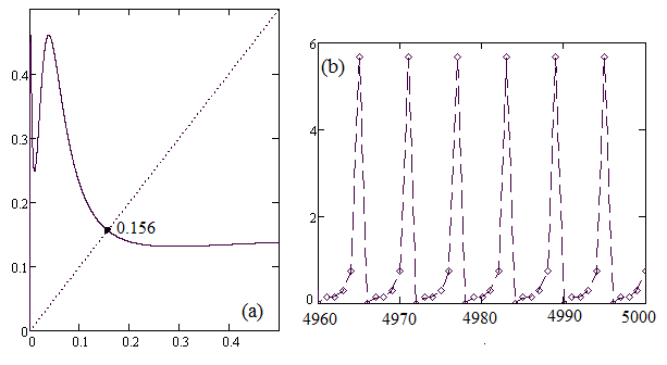
Figure 3: (a) Graph of ff; (b) Corresponding 6-cycle

The initial values that generate the 6-cycle in Figure 3 are x−1=1x_{-1}=1 and x0=0.8.x_{0}=0.8. Panel (a) shows the map f=g5∘⋯∘g0f=g_{5}\circ\cdots\circ g_{0} which is a composition of six exponential maps, together with a single stable positive fixed point that corresponds to the solution of (1) shown in Panel (b).
Refer to caption
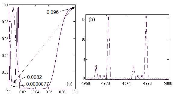
Figure 4: (a) Graphs of ff and f2f^{2}; (b) Corresponding 12-cycle

In Figure 4 the initial values are x−1=x0=1.x_{-1}=x_{0}=1. In Panel (a) the graphs of ff and f2f^{2} are shown that indicate the presence of a stable 2-cycle (the fixed point of ff is unstable in this case). Panel (b) shows the corresponding 12-cycle for (1), as required by Theorem 13 with ω=2\omega=2. We emphasize that this solution coexists stably with the 6-cycle in 3. We further note 12-cycles do not exist under the hypotheses of Corollary 9 since those hypotheses imply the stability of the fixed point of ff.

Refer to caption
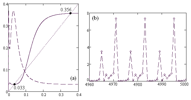
Figure 5: (a) Graphs of ff and f3f^{3}; (b) Corresponding 18-cycle

In Figure 5 the initial values are x−1=1x_{-1}=1 and x0=3.8.x_{0}=3.8. In Panel (a) the graphs of ff and f3f^{3} are shown where a stable 3-cycle is indicated that corresponds to the solution of (1) that is shown in Panel (b). As stated in Theorem 13 this is an 18-cycle since now ω=3\omega=3. This solution coexists stably with the 6-cycle and the 12-cycle above. Also note that 18-cycles do not exist under the hypotheses of Corollary 9.
Refer to caption
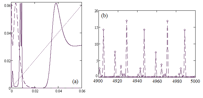
Figure 6: (a) Graphs of ff and f3f^{3}; (b) Corresponding nonperiodic solution

Finally, in Figure 6 the initial values are x−1=1x_{-1}=1 and x0=6.x_{0}=6. Panel (a) shows the graphs of ff and f3f^{3} where we can identify a pair of unstable 3-cycles where the graph of f3f^{3} crosses the identity line (in addition to the unstable fixed point of ff). The map ff then exhibits Li-Yorke type chaos. A portion of the plot of the corresponding solution of (1) is shown in Panel (b). This nonperiodic solution coexists stably with the periodic solutions mentioned above. However, nonperiodic solutions do not exist under the hypotheses of Corollary 9.

4 The even period case

When {an}\{a_{n}\} is periodic with minimal even period pp the next result shows that the sequence {tn}\{t_{n}\} is not periodic with the exception of a boundary case. This causes a fundamental change in the dynamics of (1). Once again, the quantity σ\sigma is defined by (9), i.e.

σ=−a0+a1−a2+…+ap−1.\sigma=-a_{0}+a_{1}-a_{2}+\ldots+a_{p-1}.
Lemma 14

Suppose that {an}\{a_{n}\} is a sequence of real numbers with minimal even period p≥2p\geq 2 and let {tn}\{t_{n}\} be a solution of (3). Then

tn=(t0​edn​σ+γn)(−1)nt_{n}=\left(t_{0}e^{d_{n}\sigma+\gamma_{n}}\right)^{(-1)^{n}} (20)

where the integer divisor dn=[n−n⁡(mod⁡p)]/pd_{n}=[n-n(\operatorname{mod}p)]/p is uniquely defined by each nn and

γn={∑j=1n⁡(mod⁡p)(−1)j​aj−1if ​n​(mod⁡p)≠00if ​n​(mod⁡p)=0\gamma_{n}=\left\{\begin{array}[c]{ll}\sum_{j=1}^{n(\operatorname{mod}p)}(-1)^{j}a_{j-1}&\text{if }n(\operatorname{mod}p)\not=0\\ 0&\text{if }n(\operatorname{mod}p)=0\end{array}\right. (21)

The sequence {tn}\{t_{n}\} is periodic with period pp iff σ=0\sigma=0, i.e.

a0+a2+⋯ap−2=a1+a3+⋯+ap−1.a_{0}+a_{2}+\cdots a_{p-2}=a_{1}+a_{3}+\cdots+a_{p-1}. (22)

Proof. Let {a0,a1,…,ap−1}\{a_{0},a_{1},\ldots,a_{p-1}\} be a full cycle of ana_{n} with an even number of terms. Since n=p​dn+n⁡(mod⁡p)n=pd_{n}+n(\operatorname{mod}p) for n≥1n\geq 1, expand sns_{n} in (8) to obtain

sn=dn​σ+∑j=1n⁡(mod⁡p)(−1)j​aj−1s_{n}=d_{n}\sigma+\sum_{j=1}^{n(\operatorname{mod}p)}(-1)^{j}a_{j-1}

if n⁡(mod⁡p)≠0.n(\operatorname{mod}p)\not=0. If pp divides nn so that n⁡(mod⁡p)=0n(\operatorname{mod}p)=0 then we assume that the sum is 0 and sn=dn​σ.s_{n}=d_{n}\sigma. Thus sn=dn​σ+γns_{n}=d_{n}\sigma+\gamma_{n} where γn\gamma_{n} is as defined in (21).

The σ\sigma terms have uniform signs in this case since there are an even number of terms in each full cycle of ana_{n}. Now (7) yields

tn=t0(−1)n​e(−1)n​sn=t0(−1)n​e(−1)n​(dn​σ+γn)t_{n}=t_{0}^{(-1)^{n}}e^{(-1)^{n}s_{n}}=t_{0}^{(-1)^{n}}e^{(-1)^{n}(d_{n}\sigma+\gamma_{n})}

which is the same as (20).

Next, if σ≠0\sigma\not=0 then dn​σd_{n}\sigma is unbounded as nn increases without bound so {tn}\{t_{n}\} is not periodic. But if σ=0\sigma=0 then (20) reduces to

tn=(t0​eγn)(−1)nt_{n}=\left(t_{0}e^{\gamma_{n}}\right)^{(-1)^{n}} (23)

Since the sequence γn\gamma_{n} has period p,p, the expression on the right hand side of (23) has period pp with a full cycle

t1=ea0t0,t2=t0e−a0+a1,t3=ea0−a1+a2t0,…,tp=t0e−a0+a1+⋯+(−1)p​ap−1=t0.t_{1}=\frac{e^{a_{0}}}{t_{0}},t_{2}=t_{0}e^{-a_{0}+a_{1}},t_{3}=\frac{e^{a_{0}-a_{1}+a_{2}}}{t_{0}},\ldots,t_{p}=t_{0}e^{-a_{0}+a_{1}+\cdots+(-1)^{p}a_{p-1}}=t_{0}.


By the preceding result,

t2​m\displaystyle t_{2m} =t0eγ2​med2​m​σif n=2m is even\displaystyle=t_{0}e^{\gamma_{2m}}e^{d_{2m}\sigma}\qquad\quad\text{if }n=2m\text{ is even}
t2​m+1\displaystyle t_{2m+1} =1t0​e−γ2​m+1​e−d2​m+1​σif ​n=2​m+1​ is odd\displaystyle=\frac{1}{t_{0}}e^{-\gamma_{2m+1}}e^{-d_{2m+1}\sigma}\quad\text{if }n=2m+1\text{ is odd}

Suppose that σ≠0.\sigma\not=0. If σ>0\sigma>0 then since limn→∞dn=∞\lim_{n\rightarrow\infty}d_{n}=\infty it follows that t2​mt_{2m} is unbounded but t2​m+1t_{2m+1} converges to 0, and the reverse is true if σ<0.\sigma<0. Therefore,

limm→∞t2​m\displaystyle\lim_{m\rightarrow\infty}t_{2m} =∞,limm→∞t2​m+1=0,if ​σ>0,\displaystyle=\infty,\quad\lim_{m\rightarrow\infty}t_{2m+1}=0,\quad\text{if }\sigma>0, (24)
limm→∞t2​m\displaystyle\lim_{m\rightarrow\infty}t_{2m} =0,limm→∞t2​m+1=∞,if ​σ<0.\displaystyle=0,\quad\lim_{m\rightarrow\infty}t_{2m+1}=\infty,\quad\text{if }\sigma<0. (25)
Lemma 15

Suppose that {an}\{a_{n}\} is a sequence of real numbers with minimal even period p≥2p\geq 2 and let {xn}\{x_{n}\} be a solution of (1) with initial values x−1,x0>0.x_{-1},x_{0}>0. Then limn→∞x2​n+1=0\lim_{n\rightarrow\infty}x_{2n+1}=0 if σ>0\sigma>0 and limn→∞x2​n=0\lim_{n\rightarrow\infty}x_{2n}=0 if σ<0\sigma<0.

Proof. Assume first that σ>0\sigma>0. Then by (24) limn→∞t2​n=∞\lim_{n\rightarrow\infty}t_{2n}=\infty so as in the proof of Lemma 4 limn→∞x2​n+1=0.\lim_{n\rightarrow\infty}x_{2n+1}=0. If σ<0\sigma<0 then a similar argument using (25) yields limn→∞x2​n=0\lim_{n\rightarrow\infty}x_{2n}=0 to complete the proof.  

Lemma 15 indicates that half of the terms of every solution {xn}\{x_{n}\} of (1) converge to 0 in the even period case if σ≠0.\sigma\not=0. We now consider what happens to the other half.

Lemma 16

Let {un}\{u_{n}\} be the solution of

un+1=un​ea2​n+1−unu_{n+1}=u_{n}e^{a_{2n+1}-u_{n}} (26)

and {wn}\{w_{n}\} be the solution of

wn+1=wn​ea2​n+2−wn.w_{n+1}=w_{n}e^{a_{2n+2}-w_{n}}. (27)

(a) The sequence {xn}\{x_{n}\} with x2​n=unx_{2n}=u_{n} and x2​n+1=0x_{2n+1}=0 is a solution of (1).

(b) The sequence {xn}\{x_{n}\} with x2​n=0x_{2n}=0 and x2​n+1=wnx_{2n+1}=w_{n} is a solution of (1).

Proof. (a) Let {un}\{u_{n}\} be a solution to (26) from initial value u0>0u_{0}>0. If x0=u0x_{0}=u_{0} and x1=0x_{1}=0, then

x2=x0​ea1−x0−x1=u0​ea1−u0=u1x_{2}=x_{0}e^{a_{1}-x_{0}-x_{1}}=u_{0}e^{a_{1}-u_{0}}=u_{1}

and

x3=x1​ea2−x2−x1=0x_{3}=x_{1}e^{a_{2}-x_{2}-x_{1}}=0

Inductively, if x2​k=ukx_{2k}=u_{k} and x2​k+1=0x_{2k+1}=0 for some k≥1k\geq 1 then

x2​k+2=x2​k​ea2​k+1−x2​k−x2​k+1=uk​ea2​k+1−uk=uk+1x_{2k+2}=x_{2k}e^{a_{2k+1}-x_{2k}-x_{2k+1}}=u_{k}e^{a_{2k+1}-u_{k}}=u_{k+1}

and

x2​k+3=x2​k+1​ea2​k+2−x2​k+1−a2​k+2=0x_{2k+3}=x_{2k+1}e^{a_{2k+2}-x_{2k+1}-a_{2k+2}}=0

which proves (a).

(b) Let {wn}\{w_{n}\} be a solution to (27) from initial value w0>0w_{0}>0. If x0=0x_{0}=0 and x1=w0x_{1}=w_{0}, then

x2=x0​ea1−x0−x1=0x_{2}=x_{0}e^{a_{1}-x_{0}-x_{1}}=0

and

x3=x1​ea2−x2−x1=w0​ea2−w0=w1x_{3}=x_{1}e^{a_{2}-x_{2}-x_{1}}=w_{0}e^{a_{2}-w_{0}}=w_{1}

Inductively, if x2​k=0x_{2k}=0 and x2​k+1=wkx_{2k+1}=w_{k} for some k≥1k\geq 1 then

x2​k+2=x2​k​ea2​k+1−x2​k−x2​k+1=0x_{2k+2}=x_{2k}e^{a_{2k+1}-x_{2k}-x_{2k+1}}=0

and

x2​k+3=x2​k+1​ea2​k+2−x2​k+1−a2​k+2=wk​ea2​k+2−wk=wk+1x_{2k+3}=x_{2k+1}e^{a_{2k+2}-x_{2k+1}-a_{2k+2}}=w_{k}e^{a_{2k+2}-w_{k}}=w_{k+1}

which proves (b).  

The next result is proved in [8].

Lemma 17

Consider the first-order difference equation

yn+1=yn​eαn−yny_{n+1}=y_{n}e^{\alpha_{n}-y_{n}} (28)

where αn\alpha_{n} is a sequence of real numbers with period qq. If 0<αn<20<\alpha_{n}<2 then (28) has a globally asymptotically stable solution {yn∗}\{y_{n}^{\ast}\} with period qq such that

∑i=1qyi∗=∑i=1qαi.\sum_{i=1}^{q}y_{i}^{\ast}=\sum_{i=1}^{q}\alpha_{i}.
Theorem 18

Let {an}\{a_{n}\} be periodic with minimal even period p≥2p\geq 2 and let σ\sigma be as defined in (9).

(a) If σ>0\sigma>0 and 0<a2​k−1<20<a_{2k-1}<2 for k=1,2,…​p/2k=1,2,\ldots p/2 then (1) has a globally attracting periodic solution {x¯n}\{\bar{x}_{n}\} with period pp such that x¯2​n−1=0\bar{x}_{2n-1}=0 and x¯2​n\bar{x}_{2n} is a sequence of period p/2p/2 satisfying the equality

∑i=1p/2x¯2​i−2=∑i=1p/2a2​i−1.\sum_{i=1}^{p/2}\bar{x}_{2i-2}=\sum_{i=1}^{p/2}a_{2i-1}.

(b) If σ<0\sigma<0 and 0<a2​k−2<20<a_{2k-2}<2 for k=1,2,…​p/2k=1,2,\ldots p/2 then (1) has a globally attracting periodic solution {x¯n}\{\bar{x}_{n}\} with period pp such that x¯2​n=0\bar{x}_{2n}=0 and x¯2​n−1\bar{x}_{2n-1} is a sequence of period p/2p/2 satisfying the equality

∑i=1p/2x¯2​i−1=∑i=1p/2a2​i−2.\sum_{i=1}^{p/2}\bar{x}_{2i-1}=\sum_{i=1}^{p/2}a_{2i-2}.

Proof. We prove part (a) and part (b) is demonstrated similarly. By Lemma 17 the equation in (26) has a periodic solution of period p/2p/2 given by {ui∗}\{u_{i}^{\ast}\} with 0≤i≤p/2−10\leq i\leq p/2-1. By Lemma 16, the sequence {u0∗,0,u1∗,0,⋯,up/2−1∗,0}\{u_{0}^{\ast},0,u_{1}^{\ast},0,\cdots,u_{p/2-1}^{\ast},0\} is a pp periodic solution of (1) This means that x¯2​n−1=0\bar{x}_{2n-1}=0 and x¯2​n=ui∗\bar{x}_{2n}=u_{i}^{\ast} with

∑i=1p/2x¯2​i−2=∑i=1p/2ui∗=∑i=1p/2a2​i−1.\sum_{i=1}^{p/2}\bar{x}_{2i-2}=\sum_{i=1}^{p/2}u_{i}^{\ast}=\sum_{i=1}^{p/2}a_{2i-1}.

Let the even indexed terms of the solution {xn}\{x_{n}\} be defined as in (15) and for each n≥0n\geq 0, define

Fn​(x)=x​eρn−x−μn​x​e−xF_{n}(x)=xe^{\rho_{n}-x-\mu_{n}xe^{-x}}

Then Fn​(un∗)=un+1∗F_{n}(u_{n}^{\ast})=u_{n+1}^{\ast}. Now observe that with ξn=Fn∘Fn−1∘⋯∘F0\xi_{n}=F_{n}\circ F_{n-1}\circ\cdots\circ F_{0}

Fn(yn)=Fn(Fn−1(yn−1))=Fn(Fn−1(⋯F0(y0))⋯)=ξn(y0)F_{n}(y_{n})=F_{n}(F_{n-1}(y_{n-1}))=F_{n}(F_{n-1}(\cdots F_{0}(y_{0}))\cdots)=\xi_{n}(y_{0})

Also note that

|ξn′​(y0)|=|∏i=0neρi−yi−μi​yi​e−yi​(1−μi​yi​e−yi)​(1−yi)||\xi_{n}^{\prime}(y_{0})|=\left|\prod_{i=0}^{n}e^{\rho_{i}-y_{i}-\mu_{i}y_{i}e^{-y_{i}}}(1-\mu_{i}y_{i}e^{-y_{i}})(1-y_{i})\right|

Since μn→0\mu_{n}\rightarrow 0, for sufficiently large NN, 0<(1−μn​yn​e−yn)≤10<(1-\mu_{n}y_{n}e^{-y_{n}})\leq 1 for n≥Nn\geq N. Then there exists a constant M>0M>0 so that

|∏i=0n(1−μi​yi​e−yi)|≤|∏i=0N(1−zi+1)|≤M\left|\prod_{i=0}^{n}(1-\mu_{i}y_{i}e^{-y_{i}})\right|\leq\left|\prod_{i=0}^{N}(1-z_{i+1})\right|\leq M

Proceeding now as in the proof of Lemma 7, if we let m=[n/2]m=[n/2], we can find constants K>0K>0 and δ∈(0,1)\delta\in(0,1) so that

|∏i=0n(1−yi)|≤K​δm\left|\prod_{i=0}^{n}(1-y_{i})\right|\leq K\delta^{m}

Therefore,

|ξn′​(y0)|=yn+1y0​|∏i=0n(1−μi​yi​e−yi)​(1−yi)|≤βα​K​M​δm|\xi_{n}^{\prime}(y_{0})|=\frac{y_{n+1}}{y_{0}}\left|\prod_{i=0}^{n}(1-\mu_{i}y_{i}e^{-y_{i}})(1-y_{i})\right|\leq\frac{\beta}{\alpha}KM\delta^{m}

Finally,

|yn+1−un+1∗|=|Fn​(yn)−Fn​(un∗)|=|ξn​(y0)−ξn​(u0∗)|=|ξ′​(w)|​|y0−u0∗|≤bα​K​M​δm|y0−u0∗|→0|y_{n+1}-u_{n+1}^{\ast}|=|F_{n}(y_{n})-F_{n}(u_{n}^{\ast})|=|\xi_{n}(y_{0})-\xi_{n}(u_{0}^{\ast})|=|\xi^{\prime}(w)||y_{0}-u_{0}^{\ast}|\leq\frac{b}{\alpha}KM\delta^{m}|y_{0}-u_{0}^{\ast}|\rightarrow 0

as n→∞n\rightarrow\infty which completes the proof.  

Remark 19

1. In Theorem 18(a) the even-indexed terms a2​ka_{2k} are not restricted to (0,2) as long as σ>0\sigma>0, i.e.

a1+a3+⋯+ap−1>a0+a2+⋯+ap−2a_{1}+a_{3}+\cdots+a_{p-1}>a_{0}+a_{2}+\cdots+a_{p-2}

This imposes an upper bound a2​k<2​(p/2)=pa_{2k}<2(p/2)=p for each kk but clealy some a2​ka_{2k} may exceed 2. Similarly, in (b) the odd-indexed terms are not restricted to (0,2) as long as σ<0\sigma<0.

2. Note that 2​p2p is not a minimal period for {x¯n}.\{\bar{x}_{n}\}. For example, if p=4p=4 with a1=a3a_{1}=a_{3} and 2​a1>a0+a22a_{1}>a_{0}+a_{2} (so that σ>0\sigma>0) then x¯2​n−1\bar{x}_{2n-1} satisfies (28) with constant ρn.\rho_{n}. In this case, Lemma 17 yields a globally asymptotically stable fixed point for (28), and thus a globally attracting period two solution for (1).

Figure 7 illustrates Theorem 18 with p=4p=4 and

a0=1.4,a1=1.8,a2=1.6,a3=0.3a_{0}=1.4,\quad a_{1}=1.8,\quad a_{2}=1.6,\quad a_{3}=0.3
Refer to caption
Figure 7: Solutions converging to a single 4-cycle with parameter period p=4

In the boundary special case σ=0\sigma=0, the solutions of (1) have entirely different dynamics that resemble the odd period case. Indeed, the next result is similar to Theorem 13.

Corollary 20

Suppose that {an}\{a_{n}\} is periodic with minimal even period pp and σ=0.\sigma=0. Let ff be the interval map in Lemma 11 where t0>0t_{0}>0 is a fixed real number and tkt_{k} is given by (7)-(8) for k≥1k\geq 1.

(a) If ss is a periodic point of ff with period ω\omega then all solutions of (1) with initial values x−1=sx_{-1}=s and x0=t0​s​e−sx_{0}=t_{0}se^{-s} (i.e. (x−1,x0)(x_{-1},x_{0}) is on the curve g0g_{0}) have period p​ω.p\omega.

(b) If the map ff has a non-periodic point, then (1) has a non-periodic solution.

(c) If ff has a period-three point then (1) has periodic solutions of period p​npn for all positive integers nn as well as chaotic solutions in the sense of Li-Yorke [4].

Proof. By Lemma 14 {tn}\{t_{n}\} has period pp so the application of Lemma 12 completes the proof.  

If p=2p=2 in the above corollary then a0=a1a_{0}=a_{1} (because σ=0\sigma=0) so the sequence {an}\{a_{n}\} is constant, i.e. it has mimimal period 1 not 2. The behavior described in the corollary is indeed that which is observed for the constant parameter case; see [3] for a discussion of the stability of the variety of solutions mentioned above, which is of the same type as noted in Remark 10.

5 Summary and future directions

We used a semiconjugate factorization of (1) to investigate its dynamics. Semiconjugate factorizations for difference equations of exponential type are not generally known (unlike linear equations) but fortunately we have one for (1). As we see above, the decomposition of (1) into the system (5)-(6) of first-order equations makes it clear why the solutions of (1) behave differently in a fundamental way depending on whether the period of {an}\{a_{n}\} is odd or even: in the former case the sequence {tn}\{t_{n}\} is periodic, hence bounded while the latter case {tn}\{t_{n}\} is unbounded when σ≠0.\sigma\not=0.

The main results of this paper are Corollary 9 and Theorem 13 that discuss the dynamics of solutions if pp is odd and Theorem 18 if pp is even. Corollary 9 and Theorem 13 show that (1) has multistable coexisting solutions, including non-periodic and chaotic solutions if the amplitude of the parameter sequence ana_{n} is unrestricted. Theorem 18 indicates a completely different dynamics where globally stable limit cycles occur when ana_{n} is restricted to the interval (0,2). Another of our main results is Theorem 8 that extends previous special cases in [2] and [3]. Further, Corollary 9 is a consequence of Theorem 8.

An extension of Theorem 18 that includes non-periodic solutions when ana_{n} exceeds 2 for some indices nn is expected and may be of future interest. Such an extension evidently proves the existence of asymptotically stable non-periodic solutions, including chaotic solutions for (1) when σ≠0\sigma\not=0.

A natural extension of the above results is not obvious for higher order versions of (1) such as

xn+1=xn−1​ean−xn−xn−kx_{n+1}=x_{n-1}e^{a_{n}-x_{n}-x_{n-k}} (29)

For instance, (29) may have unbounded solutions if k≥2k\geq 2 and exhibits different dynamics than (1). Further, known semicongjugate factorizations for (29) decompose it into a factor equation with order at least 2 if k≥2k\geq 2; see [9]. Such an equation is less tractable than the first-order case studied above. A detailed study of difference equations such as (29) and similar with periodic {an}\{a_{n}\} may yield interesting and possibly unexpected results.

References

  • [1] Elaydi, S.N., Discrete Chaos, 2nd ed., Chapman & Hall/CRC, Boca Raton, 2008
  • [2] Franke, J.E., Hoag, J.T. and Ladas, G., Global attractivity and convergence to a two-cycle in a difference equation, J. Difference Eq. Appl. 5, 203-209, 1999
  • [3] Lazaryan, N. and Sedaghat, H., Extinction, periodicity and multistability in a Ricker model of Stage-structured populations, J. Difference Eq. Appl., 2016, DOI: 10.1080/10236198.2015.1123707
  • [4] Li, T-Y and Yorke, J.A., Period three implies chaos, Amer. Math. Monthly 82, 985-992, 1975
  • [5] Liz, E. and Pilarczyk, P., Global dynamics in a stage-structured discrete-time population model with harvesting, J. Theor. Biol. 297, 148-165, 2012
  • [6] Luis, R., Elaydi, S., Oliveira, H., Stability of a Ricker-type competition model and the competitive exclusion principle, J. Biol. Dyn. 5, 636-660, 2011
  • [7] Ricker, W.E., Stock and recruitment, Journal of Fish Research Board of Canada 11, 559-623, 1954
  • [8] Sacker, R., A Note on Periodic Ricker Maps. J. Difference Eq. and Appl., 13, 89-92, 2007
  • [9] Sedaghat, H., Form Symmetries and Reduction of Order in Difference Equations, CRC Press, Boca Raton, 2011
  • [10] Smital, J., Why it is important to understand the dynamics of triangular maps, J. Difference Eq. and Appl. 14, 597-606, 2008
  • [11] Zipkin, E.F., Kraft, C.E., Cooch, E.G., and Sullivan, P.J., When can efforts to control nuisance and invasive species backfire? Ecol. Appl. 19, 1585-1595, 2009.