Supermassive Black Holes with High Accretion Rates in Active Galactic Nuclei.
VI. Velocity-resolved Reverberation Mapping of H LineNote: Received 2015 December 22; accepted 2016 February 3
Abstract
In the sixth of the series of papers reporting on a large reverberation mapping (RM) campaign of active galactic nuclei (AGNs) with high accretion rates, we present velocity-resolved time lags of H emission lines for nine objects observed in the campaign during 20122013. In order to correct the line-broadening caused by seeing and instruments before the analysis of velocity-resolved RM, we adopt Richardson-Lucy deconvolution to reconstruct their H profiles. The validity and effectiveness of the deconvolution are checked out by Monte Carlo simulation. Five among the nine objects show clear dependence of time delay on velocity. Mrk 335 and Mrk 486 show signatures of gas inflow whereas the clouds in the broad-line regions (BLRs) of Mrk 142 and MCG +06-26-012 tend to be radial outflowing. Mrk 1044 is consistent with the case of virialized motions. The lags of the rest four are not velocity-resolvable. The velocity-resolved RM of super-Eddington accreting massive black holes (SEAMBHs) shows that they have diversity of the kinematics in their BLRs. Comparing with the AGNs with sub-Eddington accretion rates, we do not find significant differences in the BLR kinematics of SEAMBHs.
Subject headings
accretion, accretion disks – galaxies: active – quasars: supermassive black holesI. Introduction
Active galactic nuclei (AGNs) are very energetic sources powered by accretion onto supermassive black holes (SMBHs) in centers of their host galaxies. In optical/ultraviolet (UV) spectra of AGNs, the most prominent features are plenty of broad emission lines whose full-width-half-maximum (FWHM) spans from to (e.g., Schmidt 65, Osterbrock & Mathews 50, Boroson & Green 12, Sulentic et al. 70, Shen et al. 68 and references therein). These emission lines originate from the gas in the broad-line regions (BLRs), which is photoionized by the continuum from central engines [49, 30]. In the past decades, reverberation mapping (RM, e.g., Bahcall et al. 1, Blandford & McKee 9, Peterson et al. 56) has become the mainstay in studying the kinematics and geometry of BLRs, as well as in measuring the masses of SMBHs in the centers of AGNs. It discerns the BLRs in time domain, instead of spatially, by monitoring spectroscopically the response of broad emission lines to the variations of continuum fluxes. RM observation has been carried out for more than 50 AGNs by many different groups [56, 59, 36, 57, 58, 35, 6, 7, 15, 60, 61, 4, 3, 2, 18, 74, 19, 67], and measures successfully their time delays between the variations of continuum and emission lines. Enormous progress has been made in understanding the BLRs through RM observations (see recent reviews, e.g., Gaskell 22, Popović 64, Netzer 48).
However, a main objective of RM is to reconstruct the so-called velocity-delay map (also known as “transfer function”), which is a function of the time lag and line-of-sight velocity of BLR gas, instead of only getting an averaged time lag of the emission line [9, 32, 33]. Due to the requirements of homogeneous sampling, accurate calibration, excellent signal-to-noise (S/N) ratios and high resolution for the reconstruction of velocity-delay maps [33], a relatively simpler analysis, that measuring the time lags of emission line as a function of line-of-sight velocity (velocity-resolved time lags), have been applied to about a dozen of AGNs (e.g., Bentz et al. 6, Bentz et al. 7, Bentz et al. 8, Denney et al. 15, Denney et al. 16, Grier et al. 28) and reveal the kinematics and geometry of their BLRs. It is very similar to the projection of velocity-delay map on the velocity axis. Furthermore, some more recent works have recovered the velocity-delay maps in several AGNs successfully by maximum entropy methods [8, 28] or Markov Chain Monte Carlo method [53, 55].
Since 2012, we have started a large RM campaign to monitor a sample of AGNs with high accretion rates, especially super-Eddington accreting massive black holes (SEAMBHs). The goal of the campaign is to understand better the super-Eddington accretion onto black holes, the BLR physics and their potential as a new probe of cosmological distance [75, 74]. The observations and light curves of H emission line in the first year (2012-2013) have been published in Du et al. (2014, hereafter Paper I) and Wang et al. (2014, hereafter Paper II), and the time lags of their Fe ii emission are presented in Hu et al. (2015, hereafter Paper III). The second stage of the campaign (2013-2014) have also been published in Du et al. (2015, hereafter Paper IV). These samples provide us opportunity to take a close look at the kinematics and geometry of the BLRs in high accretion rate AGNs. In particular, the well-known BLR radius-luminosity correlation ( relationship, see Kaspi et al. 36, Bentz et al. 5) is reported to show some dependence on accretion rate (paper IV), implying that the BLRs are indeed different in AGNs with high accretion rates from the normal ones.
This paper presents the velocity-resolved time lags of the sources in the first year of our SEAMBH campaign. Section II gives a short review of the observation and data reduction. Section III describes in detail the deconvolution method we used to correct line-broadening caused by seeing and instruments, as well as a Monte Carlo simulation to evaluate the effectiveness of the correction. In this section, we also show a comparison of the H profiles before and after the deconvolution procedures. The obtained velocity-resolved time lags are provided in Section IV. Section V gives a brief discussion and Section VI a summary of the new results.

II. Observations and Data Reduction
Details of the target selection, the instruments, the observation and the procedures of data reduction of the campaign in 2012-2013 (hereafter SEAMBH2012) have been presented by Paper I and II. For completeness, in this section, we provide a brief summary of the main points.
II.1. Sample Selection
The targets selected for SEAMBH2012 are mainly narrow-line Seyfert 1 galaxies (NLS1s, see, e.g., Osterbrock & Pogge 51), which, as a peculiar group of AGNs, are suspected to be candidates of SEAMBHs. The characteristics of NLS1s are: 1) narrow Balmer lines (FWHM km s-1), 2) strong optical Fe ii emission (relative to ), 3) weak [O iii] lines and 4) steep hard X-ray spectrum [51, 10]. We selected NLS1s with extremely steep 210 keV continuum, which is known to anti-correlate with accretion rates (Wang et al. 2004). For the SEAMBH2012 sample, we monitored nine NLS1s successfully, whose names and coordinates are summarized in Table 1 of Paper II.
II.2. Spectroscopy and Data Reduction
All of the spectroscopic observations were carried out with the Yunnan Faint Object Spectrograph and Camera which is mounted on the Lijiang 2.4-m telescope at the Yunnan Observatories of the Chinese Academy of Sciences. To obtain spectra with highly accurate flux calibration, we oriented the long slit to take the spectra of the object and a nearby non-varying comparison star (used as standard) simultaneously. This method was applied to RM campaign early in [46] and [36]. In SEAMBH2012, we fixed the slit width to 2″.5 given the seeing conditions, and used Grism 14 with a resolution of 92 Å mm-1 and a wavelength coverage of 3800-7200Å which yields () in dispersion direction finally. All of the spectroscopic data were reduced with IRAF v2.16 and the flux was calibrated by comparing spectra of the targets with those of the comparison stars exposured in the slit. Readers are referred to Paper I for more details.
| Object | Stellar Template | Spectral Typea |
|---|---|---|
| Mrk 335 | HD 77818 | K1 IV |
| Mrk 1044 | HD 173399 | G5 IV |
| IRAS 04416+1215 | HD 10307 | G1.5 V |
| Mrk 382 | SAO 126242 | F7 Vw |
| Mrk 142 | HD 142373 | F8 Ve… |
| MCG +06-26-012 | HD 131156 | G8 V |
| IRAS F12397+3333 | HD 118100 | K5 Ve |
| Mrk 486 | HD 20618 | G6 IV |
| Mrk 493 | HD 118100 | K5 Ve |
Note. — Name and spectral type of the selected template for the comparison stars.
III. Correction for Line-broadening
In spectroscopic observation, the line-broadening (), which is caused by seeing and instruments (e.g., grism or grating), influences the observed profiles of emission lines. Although the instrumental settings remain the same during observations, the seeing varies nights by nights (FWHM of the point-spread functions in SEAMBH2012 is generally from 1″.2 to 2″.5, while the width of slit is fixed to 2″.5 which is wider than seeing), and in each night changes as well. Furthermore, the mis-centering of objects and comparison stars in the slit is not a constant in different nights. This causes that each spectrum have slightly different shift in dispersion direction. Fortunately, we are also able to estimate the shifts from the spectra of comparison stars so that we can correct this automatically by deconvolution.
The observed H profile of is a convolution of its intrinsic profile and the line-broadening function , namely
| (1) |
Variations of does not change the integrated flux of H emission line, however, it blurs and further influences the velocity-resolved time series analysis. It is thus expected to correct the line-broadening of H profiles before the velocity-resolved RM analysis, especially for those objects with relatively narrow H lines (FWHM 1000 – 2000km/s, comparing to the instrumental broadening of 500km/s estimated in Paper I) in our SEAMBH2012 observation. Fortunately, the spectra of comparison stars in the same slit during spectroscopic exposures can be employed to estimate accurately in light of that the FWHM of absorption lines in stellar spectra ( 10) is much narrower than the line-broadening. An efficient way to perform such a correction is the well-known Richardson-Lucy algorithm [63, 44] which can deconvolve from so as to recover .
Figure 1 shows the sketch of procedures for line-broadening correction. We first estimate the broadening function of exposure via fitting the spectrum of comparison star in each night by a stellar template, then use the obtained to correct the broadening of H profile in the observed spectra through Richardson-Lucy deconvolution algorithm. Finally, we can get the broadeing-corrected profile .
III.1. Richardson-Lucy Deconvolution
Richardson-Lucy (R-L) deconvolution algorithm is a Bayesian-based iterative technique commonly used for recovering signal blurred by a known response. It has been widely adopted to improve the spatial resolution of images from Hubble Space Telescope (HST, e.g., Lauer et al. 40, Snyder et al. 69, Lauer et al. 41, Gebhardt et al. 25, Schmitt & Kinney 66, Kormendy & Bender 39, Farrah et al. 20, Rest et al. 62, Lauer et al. 42 and the references therein), and to correct the instrumental broadening in spectroscopic data such as ultraviolet spectra from Goddard High Resolution Spectrograph on HST (e.g., Wahlgren et al. 73, Brandt et al. 13, Bomans et al. 11) or X-ray spectroscopy measurements of heavy elements [21]. Even recently, [47] used it in data analysis of integral field spectrograph from Gemini. To our knowledge, this is the first application of such technique to the correction of instrumental broadening in spectra from RM observation.
We do not repeat the details of R-L deconvolution here, but just give a brief description (readers may refer to original papers [63] and [44]). In short, if is the -th estimate of the intrinsic profile in the iterative sequence, the -th estimate is obtained by
| (2) |
where
| (3) |
Similar to the widely used equidistribution of ignorance in Bayes’s postulate, we assume a uniform distribution as the initial guess of intrinsic profile, so that . After a certain number (see Section III.3) iterations, the intrinsic profile can be recovered effectively.

III.2. Line-broadening Function
During the spectroscopic exposures, we oriented the slit in order to simultaneously include the target and a nearby comparison star for their spectra (an object-star pair). It enables us to obtain of the object synchronously from the comparison star in the pair. To estimate the broadening function, we use the direct pixel-fitting method similar to [27] and [31]. The observed spectrum of comparison star is modeled by a stellar template spectrum convolved by the broadening function:
| (4) |
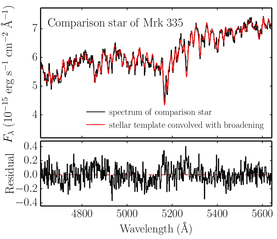
Here, is a polynomial accounted for large-scale mismatch in the continuum shape of the comparison star and template. In this work, we assume a Gaussian function and select the most similar stellar spectrum as the template of comparison star from the Indo-U.S. Library of Coudé Feed Stellar Spectra11 1 http://www.noao.edu/cflib/ [72]. The selected templates for the comparison stars are listed in Table 1. In order to get the line-broadening function close enough to , we set the fitting window to 4500Å-5500Å in rest frame of the objects. Prior to the fitting, the consecutive exposures of the object-star pair in each night are combined so as to provide high S/N ratio. The best values of FWHM and shift in are determined by fitting the combined spectrum of the comparison star in each night via Levenberg-Marquardt algorithm.
An example of individual-night spectrum of the comparison star and the best model for Mrk 335 is shown in Figure 2. The distributions of FWHM and shift of during the observation of Mrk 335 are shown in Figure 3. The FWHM, on average, is consistent with the mean value of 500km s-1 estimated in Paper I. However, through the fitting here, we are able to measure the broadening function in each individual night. For the other objects, the distributions of the broadening are similar to the case of Mrk 335, so we do not show them repeatedly here. It should be noted that, although SEAMBHs generally have weak [O iii], we can still try to estimate from the [O iii] line in several objects with relatively strong and intrinsicly narrow [O iii] (e.g., Mrk 382) by comparing its width to the value of spectra with higher resolution [77], if we assume the narrow lines do not vary with time. The obtained from [O iii] is consistent with the values estimated by the fitting here, and the differences are km s-1 averagely.
After getting in each night (for each target), we reconstruct by applying R-L deconvolution to the observed spectra of the objects.

III.3. Iteration Number
The termination of iterations is one of the core issues in R-L deconvolution. Too few iterations are insufficient for reconstruction of the original signal, while an excess of iterations magnifies high-frequency noise and even produces nonsense results [44]. Here, a simple Monte Carlo approach is used to determine the appropriate number for terminating the iterations.
For each object, we first construct an Gaussian, with the same FWHM and equivalent width (EW) of H in the observed mean spectra, where the mean broadening of 500 km s-1 estimated in Paper I have been subtracted, as the artificial intrinsic spectrum. This artificial intrinsic spectrum is used to generate a mock observed spectrum in each individual night by convolving with obtained from the fitting in Section III.2 and adding random noises with the same level of S/N as the truly observed spectrum. Then, we select the iteration number which can get the best reconstruction (with the smallest ) of the artificial intrinsic spectrum by de-convolving from the mock as the optimal number of iterations. The mock is generated 20 times for each spectrum, and the median value of the optimal numbers of iterations obtained by the above procedure is chosen as the final iteration number of the deconvolution.
III.4. Host Galaxy Subtraction
The spectra of AGNs and comparison stars are smeared by the same broadening function every night since both of them are point sources. However, the host galaxies of the objects are extended and their spectra are affected by broadening which is different from those of comparison stars. Therefore, before de-convolving the spectra of AGNs with the broadening function obtained from the comparison stars in Section III.2, the contribution of host galaxies should be removed. Paper III has already decomposed the spectra and extracted the contribution of host galaxies by fitting scheme. We simply subtract those host contributions, which we got in Paper III, from the spectra of objects before the procedures of deconvolution to avoid potential influence of different broadening in host galaxies.


III.5. Monte Carlo Simulation on Deconvolution
We make use of Monte Carlo simulation to evaluate the robustness of reconstructing the intrinsic profile of H line through the R-L deconvolution. We first create an artificial AGN spectrum by including (a) a power-law continuum; (b) Fe ii emission and broad He ii; (c) narrow emission lines of H and [O iii]4959,5007 and (d) a broad component of . The components here are almost the same as the model we used in Paper III except for the absence of host galaxy contribution (host does not influence the profiles of H in the simulation). We set the FWHM and EW of H in the artificial AGN spectrum to 1200km/s and 100Å (see Figure 4), respectively, which are the typical values in the present sample. In order to test the precision of recovery by the deconvolution in the cases with various broadening and S/N ratio, we broaden the artificial spectrum by different broadening function and plus stochastic noise to generate the simulated observed spectra. In the meantime, we select a stellar spectral template (HD 44951 used here) from the Indo-U.S. Library and broaden it with the same broadening as the AGN spectrum and plus noise as well. We take the simulated observed AGN and star spectra as the input of the procedures in Section III, and then compare the profiles of H in the output reconstructed spectra to those of the original artificial AGN spectra.
To elaborate the comparison of profiles between the spectra before and after the deconvolution procedures, we define full width at (20%, 50%, 80%) of maximum as (W20, W50, W80), and centers at (20%, 50%, 80%) of maximum as (C20, C50, C80) to characterize the profiles of H (please see Figure 5 for their definition). (W20, W50, W80) evaluate the width of emission line at different height, while (C20, C50, C80) show the shifts at the corresponding levels (see figure 5). Here, W50 is just simply FWHM in the common sense. The comparison of emission-line profiles before and after the deconvolution in the Monte Carlo simulations is shown in Figure 6. Generally speaking, the deconvolution can recover the profile of H correctly. (W20, W50, W80) and (C20, C50, C80) of the reconstructed H profiles are consistent with the value of the input artificial AGN spectrum in the cases with high S/N ratios. The reconstruction is more successful in the cases with narrower broadening function and higher S/N ratio, especially when the FWHM of broadening is narrower than the input H profile. The widths of H in the observed spectra of SEAMBH2012 are 1000 2000 km s-1, while the broadening is only 500 km s-1. And the S/N ratio of spectra in SEAMBH2012 is generally higher than 20. Therefore, the intrinsic profiles recovered by the deconvolution Section III is reliable.
III.6. Profiles Before and After the Deconvolution
In order to give an overall evaluation how effectively does the deconvolution work, examples of the comparison between observed and de-convolved spectra of Mrk 335 are provided in Figure 7. It is very obvious that the deconvolution procedures correct the broadening and mis-centering effect successfully. To further compare the profiles before and after the deconvolution, we measure (W20, W50, W80) and (C20, C50, C80) of H in the spectra before and after the deconvolution procedures. As an example, the values of Mrk 335 are shown in Figure 8. After the deconvolution, the widths (W20, W50, W80) of its H lines narrow down for (, , ) on average. In particular, the distribution of W80 in the reconstructed spectra becomes much narrower, which means the more serious influence caused by the broadening around the peak (the highest and narrowest part) of emission line, than in its wing part (with broader width), have been corrected effectively. Additionally, the centers at different levels (C20, C50, C80) are more concentrated than the cases before the deconvolution. The comparison before and after the deconvolution demonstrates the validity of the deconvolving procedures used in the present paper. The centers, it should be noted, do not locate on 0 km s-1 because the zero here is defined by the redshift queried from NASA/IPAC Extragalactic Database22 2 http://ned.ipac.caltech.edu/.


IV. Velocity-resolved Time Series Analysis
IV.1. Methods
The light curves and the time delays between the variations of the continuum at 5100Å and H fluxes measured by simply integrating the full extent of the emission lines have been published in Paper I and II. Paper III updated these measurements by introducing a sophisticated scheme that fit AGN continuum, host contribution in the slit and emission lines simultaneously. The updated time lags are consistent with the previous ones but have smaller uncertainties (see the comparison in Paper III). However, these time delays only stand for the radii averaged by the emissivity function of BLRs, and no information of velocity fields is carried out. In this section, we focus on the velocity-resolved analysis of delays in order to reveal the kinematics of BLR clouds in SEAMBHs.
The procedures of deconvolution in Section III have removed the varying line-broadening from the observed profiles and almost corrected the wavelength shifts caused by mis-centering. After further correcting the remanent shifts ( km s-1) using [O iii] line as our wavelength reference, the spectra are ready for velocity-resolved time series analysis. RMS (root of mean-square) spectra of the objects are obtained in the standard way from the spectra after the line-broadening correction. Similar to many previous works (e.g., Bentz et al. 6, Bentz et al. 7, Denney et al. 15, Denney et al. 17, Bentz et al. 8, Denney et al. 16, Grier et al. 28), we divide H emission line into several bins in velocity space, where each bin has equal amount of flux in the RMS spectrum. After integrating the flux of emission line in each bin, we cross-correlate the obtained individual-bin light curves to the continuum light curve at 5100Å. Due to the lack of error bars in the output spectra of deconvolution, we estimate the uncertainties of flux in the individual-bin light curves based on the differences between adjacent points using median filter as in Paper I. The interpolation cross-correlation function (ICCF; Gaskell & Sparke 24, Gaskell & Peterson 23, White & Peterson 76) is employed, and the centroid of the CCF, above 80% of the maximum cross-correlation coefficient (), is adopted as the time lags (e.g., Koratkar & Gaskell 38, Peterson et al. 58, Denney et a. 14, Bentz et al. 7, Denney et al. 16 and reference therein). The uncertainties in the measured lag time are determined through the Monte Carlo “flux randomization/random subset sampling” method described in [45] and [59, 58]. The rest-frame velocity-resolved time lags of the objects, as well as their RMS spectra created after deconvolution, are shown in Figure 9 and 10. The details of objects are discussed below.
IV.2. Individual Objects
Mrk 335. The H emission line of this object is divided into eight bins in velocity space, where each bin contains of the variable line flux in its RMS spectrum. Its velocity-resolved time series analysis (see Figure 9) demonstrates clear gradient in the delays of different velocity bins that the blueshifted part of H lags the response in its redshifted part (from days in the blue end to days in the red end). This kinematic signature is consistent with the expectation of inflow that the gas on near side is receding to the observer while the gas on opposite side is approaching. In Figure 9, we also show the result before the deconvolution. Generally speaking, the velocity-resolved time delays before and after the deconvolution are consistent with each other. However, the deconvolution-corrected result show some details, more clearly, that the longer time delays in blueshifted part vary gently while the lags in the redshifted part decrease more quickly. The before-deconvolution time lags only show uniform gradient from blue- to red-shifted velocity. In particular, the RMS spectrum before the deconvolution contains relatively stronger contribution of narrow H emission line which is caused by the varying width of narrow line (because of the changing broadening in each night), while this feature is much weaker in the RMS spectrum of the reconstructed profiles. The comparison in Figure 9 also indicates that the deconvolution procedures can recover the velocity-resolved information moderately in RM time-series analysis.
Before our observation, Mrk 335 was monitored twice in 19891996 [37, 59] and 20102011 [29], respectively. Its velocity-resoved time lags in the latter campaign have been published in [28]. It is not unexpected that the inflow signature in the velocity-resoved delays presented here is consistent with the previous measurements in 20102011 [28], given the short time interval between these two campaigns. Such a kind of signature has also been reported in the velocity-resolved delay analysis of many other sources like Arp 151 [6, 7], NGC 3516 [15, 16], Mrk 1501 [28] and PG 2130+099 [28].


Mrk 142. The velocity-resolved time delays of Mrk 142 are reported here for the first time. It was previously monitored by the LAMP collaboration [7], however the authors do not show its velocity-resolved lags perhaps due to their data quality. The observation in our campaign has more homogeneous cadence and better calibration precision. Opposite to the case of Mrk 335, Mrk 142 shows signature of outflow indicated by the shorter time lag from BLR gas in the blueshifted side of H line comparing with the gas in redshifted side. Interestingly, to our knowledge, the signature of outflow was observed distinctly by reverberation mapping in only one case, NGC 3227 [15, 16], before the detection shown here. Comparing with the low accretion rate in NGC 3227 (Denney et al. 16; Paper IV), Mrk 142 is a SEAMBH and radiation pressure acting on the ionized gas is probably the driver for the observed outflow.
Mrk 486. It also demonstrates clear signature of infalling gas as the case of Mrk 335. Except for the first bin, the response to the continuum variation in the blueshifted gas lags the response of the gas corresponding to the redshifted side.
Mrk 1044. The velocity-resolved lags of Mrk 1044 are relatively symmetric and show evidence of simple virialized motions, that high-velocity gas is located in the more central region, which is similar to the cases of NGC 5548 [15], SBS 1116+583A [7], Mrk 1310 [7], NGC 4051 [17, 16] and 3C 120 [28] in the previous works.
MCG +06-26-012. A signature of outflow is shown in this object that the time delays ( days) in the blue part of H are slightly shorter than those ( days) in the red part, however, the outflow signs are ambiguous a little bit because of the large errors. The large error bars are caused by the inhomogeneous sampling and the short monitoring period comparing with the variation in the light curves. MCG +06-26-012 is the only sub-Eddington object in the present sample (see details in Paper II).
Mrk 382. The lags in different velocity bins are undistinguished. This phenomenon has been found in other objects, such as Mrk 1310 [7], NGC5548 [7] and Mrk 290 [16]. This may be either caused by that the lag differences among the bins are smaller than their error bars (by the quality of the current data), or it could be real intrinsically that those bins have the same time lags. If the line-of-sight velocity keeps a constant in the BLR, motion of cloud are fully chaotic. This remains open for future observations with high quality data.
IRAS F12397+3333 and Mrk 493 are similar to Mrk 382.
IRAS 04416+1215. The direct integrating method in Paper I and II is failed to give the average time lag of its integrated H emission line flux. Only multi-components fitting method in Paper III is able to detect its delay. Here, we adopt the direct integrating method to measure the light curves after the division of bins and still fail to get reliable detection of its velocity-resolved lags. We divide its H into two bins and demonstrate the result here for completeness. The in the redshifted bin is only .


V. Discussions
Outflows suggested by the observation of blueshifted broad absorption lines are not rare in AGNs (e.g., Trump et al. 71, Gibson et al. 26 and reference therein). However, how do the outflows contribute to broad emission lines, especially in high accretion rate AGNs, is still subject to some debate. Considering that super-Eddington accreting AGNs probably have the strongest radiation pressure, which can provide kinetic energy to BLR gas, among the whole AGN populations, the possibilities of outflows that occur in SEAMBHs maybe doubt to be higher than sources with normal accretion rates. However, the present sample, although with its limited size, shows diverse properties of the BLR kinematics, rather than the simple outflows (there is only one from the detected four SEAMBHs, except for MCG +06-26-012 with low accretion rate). It is consistent with the fact that the observed profile of H in the present sample does not show unified signature of blueshifted asymmetry. On the other hand, there are a few objects (2 out of 4 super-Eddington AGNs) showing clear evidence for the presence of infalling gas in BLRs. Considering the fact that objects in the present sample are super-Eddington accreting AGNs, the velocity fields of the surrounding gas showing infall in kinematics are not surprising. Otherwise, a significant fraction of the accreting gas will be channelled into outflows, making fast growth of less massive black holes be suppressed. It is impossible to reach a conclusion about the pattern of velocity fields of ionised gas in the vicinity of black holes in super-Eddington accreting AGNs. We hope increases of monitored SEAMBHs and normal AGNs could clarify the patterns of the velocity fields.
VI. Conclusions
We have presented here velocity-resolved time lag measurements of nine objects observed in our SEAMBH2012 campaign. To correct the line-broadening caused by instruments and seeing, we use Richardson-Lucy deconvolution to reconstruct H profiles. The broadening function in each night is estimated by fitting the spectra of the stars observed simultaneously with stellar templates, and Monte Carlo method is adopted to test the validity of the broadening-correction procedures. We show that the Richdson-Lucy iteration is an efficient method to recover the velocity-resolved information to some extent.
All of the objects in the present sample are NLS1s with very high accretion rates except for MCG +06-26-012. Five sources among them demonstrate clear velocity-resolved time delays in their H emission lines. The velocity-resolved lags of Mrk 335 and Mrk 486 show the signature of gas infall, while the BLR clouds in Mrk 142 and MCG +06-26-012 tend to be radial outflowing. The symmetric pattern of Mrk 1044 is consistent with virialized motions. The time lags of the other four objects are not velocity-resolvable. We do not find significant differences in the BLR kinematics of SEAMBHs, comparing with sub-Eddington AGNs. Some discussions for the result of each individual object are provided in the main text. This analysis provides new insight into the geometry and kinematics of BLRs in SEAMBHs.
References
- [1] Bahcall, J. N., Kozlovsky, B.-Z., & Salpeter, E. E. 1972, ApJ, 171, 467
- [2] Barth, A. J., Bennert, V. N., Canalizo, G., et al. 2015, ApJS, 217, 26
- [3] Barth, A. J., Pancoast, A., Bennert, V. N., et al. 2013, ApJ, 769, 128
- [4] Barth. A. J., Pancoast, A., Thorman, S. J., et al. 2011, ApJ, 743, 4
- [5] Bentz, M. C., Denney, K. D., Grier, C. J., et al. 2013, ApJ, 767, 149
- [6] Bentz, M. C., Walsh, J. L., Barth, A. J., et al. 2008, ApJ, 689, L21
- [7] Bentz, M. C., Walsh, J. L., Barth, A. J., et al. 2009, ApJ, 705, 199
- [8] Bentz, M. C., Walsh, J. L., Barth, A. J., et al. 2010, ApJ, 716, 993
- [9] Blandford, R. D., & McKee, C. F. 1982, ApJ, 255, 419
- [10] Boller, T., Brandt, W. N., & Fink, H. 1996, A&A, 305, 53
- [11] Bomans, D. J., de Boer, K. S., Koornneef, J., & Grebel, E. K. 1996, A&A, 313, 101
- [12] Boroson, T. A., & Green, R. F. 1992, ApJS, 80, 109
- [13] Brandt, J. C., Heap, S. R., Beaver, E. A., et al. 1993, AJ, 105, 831
- [14] Denney, K. D., Bentz, M. C., Peterson, B. M., et al. 2006, ApJ, 653, 152
- [15] Denney, K. D., Peterson, B. M., Pogge, R. W., et al. 2009a, ApJ, 704, L80
- [16] Denney, K. D., Peterson, B. M., Pogge, R. W., et al. 2010, ApJ, 721, 715
- [17] Denney, K. D., Watson, L. C., Peterson, B. M., et al. 2009b, ApJ, 702, 1353
- [18] Du, P., Hu, C., Lu, K.-X., et al. (SEAMBH Collaboration) 2014, ApJ, 782, 45 (Paper I)
- [19] Du, P., Hu, C., Lu, K.-X., et al. (SEAMBH Collaboration) 2015, ApJ, 806, 22 (Paper IV)
- [20] Farrah, D., Rowan-Robinson, M., Oliver, S., et al. 2001, MNRAS, 326, 1333
- [21] Fister, T. T., Seidler, G. T., Rehr, J. J., et al. 2007, Phys. Rev. B, 75, 174106
- [22] Gaskell, C. M. 2009, NewAR, 53, 140
- [23] Gaskell, C. M., & Peterson, B. M. 1987, ApJS, 65, 1
- [24] Gaskell, C. M., & Sparke, L. S. 1986, ApJ, 305, 175
- [25] Gebhardt, K., Lauer, T. R., Byun, Y.-I., et al, 1996, AJ, 112, 105
- [26] Gibson, R. R., Jiang, L., Brandt, W. N., et al. 2009, ApJ, 692, 758
- [27] Greene, J. E., & Ho, L. C. 2006, ApJ, 641, 117
- [28] Grier, C. J., Peterson, B. M., Horne, K., et al. 2013, ApJ, 764, 47
- [29] Grier, C. J., Peterson, B. M., Pogge, R. W., et al. 2012, ApJ, 755, 60
- [30] Ho, L. C. 2004, ARA&A,
- [31] Ho, L. C., Greene, J. E., Filippenko, A. V., & Sargent, W. L. W. 2009, ApJS, 183, 1
- [32] Horne, K. 1994, in ASP Conf. Ser. 69, Reverberation Mapping of the Broad-Line Region in Active Galactic Nuclei, ed. P. M. Gondhalekar, K. Horne, & B. M. Peterson (San Francisco: ASP), 23
- [33] Horne, K., Peterson, B. M., Collier, S. J., & Netzer, H. 2004, PASP, 116, 465
- [34] Hu, C., Du, P., Lu, K.-X., et al. (SEAMBH Collaboration) 2015, ApJ, 804, 138 (Paper III)
- [35] Kaspi, S., Brandt, W. N., Maoz, D., et al. 2007, ApJ, 659, 997
- [36] Kaspi, S., Smith, P. S., Netzer, H., et al. 2000, ApJ, 533, 631
- [37] Kassebarm, T. M., Peterson, B. M., Wanders, I., et al. 1997, ApJ, 475, 106
- [38] Koratkar, A. P., & Gaskell, C. M. 1991, ApJS, 75, 719
- [39] Kormendy, J., & Bender, R. 1999, ApJ, 522, 772
- [40] Lauer, T. R., Faber, S. M., Groth, E. J., et al. 1993, AJ, 106, 1436
- [41] Lauer, T. R., Ajhar, E. A., Byun, Y.-I., et al. 1995, AJ, 110, 2622
- [42] Lauer, T. R., Faber, S. M., Gebhardt, K., et al. 2005, AJ, 129, 2138
- [43] Li, Y.-R., Wang, J.-M., Ho, L. C., Du, P., & Bai, J.-M. 2013, ApJ, 779, 110
- [44] Lucy, L. B. 1974, AJ, 79, 745
- [45] Maoz, D., & Netzer, H. 1989, MNRAS, 236, 21
- [46] Maoz, D., Netzer, H., Leibowitz, E., et al. 1990, ApJ, 351, 75
- [47] Menezes, R. B., Steiner, J. E. & Ricci, T. V. 2014, MNRAS, 438, 2597
- [48] Netzer, H. 2013, Physics and Evolution of Active Galactic Nuclei (Cambridge: Cambridge Univ. Press)
- [49] Osterbrock, D. E. 1989, Astrophysics of gaseous nebulae and active galactic nuclei (Mill Valley, CA: University Science Books)
- [50] Osterbrock, D. E., & Mathews, W. G. 1986, ARA&A, 24, 171
- [51] Osterbrock, D. E., & Pogge, R. W. 1985, ApJ, 297, 166
- [52] Pancoast, A., Brewer, B. J., & Treu, T. 2011, ApJ, 730, 139
- [53] Pancoast, A., Brewer, B. J., Treu, T., et al. 2012, ApJ, 754, 49
- [54] Pancoast A., Brewer, B. J., & Treu, T. 2014, MNRAS, 445, 3055
- [55] Pancoast, A., Brewer, B. J., Treu, T., et al. 2014, MNRAS, 445, 3073
- [56] Peterson, B. M., Ali, B., Horne, K., et al. 1993, PASP, 105, 247
- [57] Peterson, B. M., Berlind, P., Bertram, R., et al. 2002, ApJ, 581, 197
- [58] Peterson, B. M., Ferrarese, L., Gilbert, K. M., et al. 2004, ApJ, 613, 682
- [59] Peterson, B. M., Wanders, I., Bertram, R., et al. 1998, ApJ, 501, 82
- [60] Rafter, S. E., Kaspi, S., Behar, E., Kollatschny, W., & Zetzl, M. 2011, ApJ, 741, 66
- [61] Rafter, S. E., Kaspi, S., Chelouche, D., et al. 2013, ApJ, 773, 24
- [62] Rest, A., van den Bosch, F. C., Walter, J., et al. 2001, AJ, 121, 2431
- [63] Richardson, W. H. 1972, J. Opt. Soc. Am., 62, 55
- [64] Popović, L. Č. 2012, NewAR, 56, 74
- [65] Schmidt, M. 1963, Nature, 197, 1040
- [66] Schmitt, H. R., & Kinney, A. L. 1996, ApJ, 463, 498
- [67] Shen, Y., Horne, K., Grier, C. J., et al. 2015, arXiv:1510.02802
- [68] Shen, Y., Richards, G. T., Strauss, M. A., et al. 2011, ApJS, 194, 45
- [69] Snyder, D. L., Hammoud, A. M., & White, R. L. 1993, J. Opt. Soc. Am. A, 10, 1014
- [70] Sulentic, J. W., Marziani, P., & Dultzin-Hacyan, D. 2000, ARA&A, 38, 521
- [71] Trump, J. R., Hall, P. B., Reichard, T. A., et al. 2006, ApJS, 165, 1
- [72] Valdes, F., Gupta, R., Rose, J. A., Singh, H. P., & Bell, D. J. 2004, ApJS, 152, 251
- [73] Wahlgren, G. M., Leckrone, D. S., Shore, S. N., et al. 1991, ApJL, 377, L41
- [74] Wang, J.-M., Du, P., Hu, C., et al. (SEAMBH Collaboration) 2014, ApJ, 793, 108 (Paper II)
- [75] Wang, J.-M., Du, P., Valls-Gabaud, D., Hu, C., & Netzer, H. 2013, Phys. Rev. Lett., 110, 081301
- [76] White, R. J., & Peterson, B. M. 1994, PASP, 106, 879
- [77] Whittle, M. 1992, ApJS, 79, 49