The Launching of Cold Clouds by Galaxy Outflows II:
The Role of Thermal Conduction
Abstract
We explore the impact of electron thermal conduction on the evolution of radiatively-cooled cold clouds embedded in flows of hot and fast material, as occur in outflowing galaxies. Performing a parameter study of three-dimensional adaptive mesh refinement hydrodynamical simulations, we show that electron thermal conduction causes cold clouds to evaporate, but it can also extend their lifetimes by compressing them into dense filaments. We distinguish between low column-density clouds, which are disrupted on very short times, and high-column density clouds with much-longer disruption times that are set by a balance between impinging thermal energy and evaporation. We provide fits to the cloud lifetimes and velocities that can be used in galaxy-scale simulations of outflows, in which the evolution of individual clouds cannot be modeled with the required resolution. Moreover, we show that the clouds are only accelerated to a small fraction of the ambient velocity because compression by evaporation causes the clouds to present a small cross-section to the ambient flow. This means that either magnetic fields must suppress thermal conduction, or that the cold clouds observed in galaxy outflows are not formed of cold material carried out from the galaxy.
I. Introduction
Galaxy outflows play a key role in the history of galaxy formation [12, e.g.], driving multiphase material from deep within the densest regions of galaxies out into the rarified fringes of the circumgalactic medium. Such powerful outbursts are well observed in high-surface density galaxies over a wide range of masses and redshifts [38, 52, 25, 65, e.g.], including the ultraluminous infrared galaxies (ULIRGs) that host as much as half of the star formation in the Universe [55]. Their impact is extensive: they are believed to set the correlation between galaxy stellar mass and interstellar medium metallicity, [63, 28, 36, e.g.], they enrich the intergalactic medium with metals [53, 16, 41, 51, 64, e.g.], and they help determine the number density of faint galaxies [58, 4, e.g.].
At the same time, galaxy outflows are notoriously difficult to simulate [7, 2, 10, e.g.]. This is both because (i) the efficient cooling in the interstellar medium (ISM) makes it hard to model supernova feedback in galaxy-scale simulations, and (ii) the treatment of turbulent multiphase gas subject to radiative cooling, which can become thermally-unstable [56, e.g.] and which puts high demands on the range of spatial and temporal scales involved in the problem. Moreover, the observation of the multiphase ISM is difficult: the hot phases of the outflow have only been detected in a few instances [26, 66, 70, e.g.], and the cold phases of gas are often difficult to interpret. Nevertheless the kinematics of neutral, atomic outflows has been studied in many cases through absorption line as well as emission line measurements of Ly H, H and well as doublet lines such as [N II] 6549, 6583, [O II] 3726, 3729, and [O III] 4959, 5007 [59, 55, 71, 14, 30, 1, e.g.].
In [57], hereafter called Paper I, we performed a series of three-dimensional hydrodynamic simulations aimed at developing a better understanding of the cold-cloud hot-medium interactions needed to relate such observations to the evolution of galaxy outflows. The simulations were carried out on adaptive grids using the FLASH code [19], and tracked the evolution of spherical, K clouds impacted by hot winds of varying temperatures and speeds. For these simulations, we included optically-thin radiative cooling and designed the grid such that it tracked the clouds closely, enabling us to study their entire evolution, even for long disruption times.
From these calculations, we found that the Mach cone that forms around the cloud both damps shear instabilities and produces a streamwise pressure gradient that stretches the cloud. As a result, cold clouds in highly supersonic outflows can live substantially longer than in subsonic conditions. The calculations also followed a number of simple scaling laws for the cloud survival time and acceleration rate. From these, we could determine that clouds can travel out to distances of about 40 times the cloud radius but not much farther before becoming disrupted. Hence, it is difficult to associate K gas at distances of tens of kpc with K gas leaving the driving region of the starburst-driven outflow unless an additional physical process acts to preserve the cloud for longer.
In this second paper in this series, we focus on the impact of one such key physical process: thermal conduction, which occurs as rapid electrons from the hot surrounding medium move into the cold cloud. Previous investigations on the effect of this process on multiphase gas dates back several decades. In seminal work on thermal instabilities, [17] identified a characteristic length scale below which thermal instabilities are suppressed by conduction. This length scale stems from a basic distinction between radiative cooling, which increases proportional to volume, and conductive heat flux, which increases proportional to area. The resulting length scale [43, termed Field length by] is given by , where is the rate of thermal conduction and is the equilibrium cooling function. In other early work, [22] investigated the balance between cosmic-ray heating and cooling and found that thermal conduction plays a role in determining cloud sizes, and [9] computed the analytic mass loss rate of a nonradiating spherical cloud embedded in a hot plasma, both for classical conduction, as well as saturated conduction, in which the electrons stream into the clouds at their thermal speed.
More recently, [43] and [3] worked out analytic solutions for steady evaporation and condensation of isolated cold clouds in hot plasmas, and found the conditions under which a steady state is reached. In related work, [11] provided analytic solutions for the saturated (flux-limited) thermal evaporation of spherical clouds allowing the thermal conductivity to change continuously from a diffusive to a saturated form, in a manner usually employed only in numerical calculations. [46] revisited the analytic treatment of cold clouds in hot media and argued that thermal evaporation of cold gas by the hot coronae of galaxies can explain the surface brightness properties of elliptical galaxies and their active galactic nuclei. [75] analytically modeled the dynamics of cool clouds in hot winds including thermal conduction, varying the parameters of the problem, and obtaining general constraints on ram pressure acceleration by comparing velocities, column densities, and temperatures with observations
From a numerical perspective, [67, 68] simulated the conductive evaporation of spherical clouds embedded in a stationary and a moving ambient medium, respectively. [37] also presented high-resolution hydrodynamical models of warm ionized clouds embedded in a wind, and compared to the OVI and X-ray properties of galaxy outflows, but their simulations were limited to relatively short times and yielded fairly short lifetimes of the warm clouds. [48] performed 2.5-D MHD simulations of a shock impacting on an isolated gas cloud, including anisotropic thermal conduction and radiative cooling. Other efforts to model cloud-wind interactions in the interstellar medium include [29], [34], [24], [44, 18], [49], [60], [50], [27], [33], [42], and [54].
Most related to our current work is [49]. Using the same code as we do, the FLASH code, they investigated the competition between radiative cooling and thermal conduction during the evolution of spherical clouds exposed to a planar shock wave. In 3D simulations, they explored two cases, albeit with very limited spatial resolution. In case (i) with and an exterior Mach number of 30, radiative losses dominated the evolution of the shocked cloud, which fragmented into cold, dense, and compact filaments surrounded by a hot corona that was ablated by the thermal conduction. In case (ii) with and an exterior Mach number of 50, thermal conduction dominated the evolution of the shocked cloud, which evaporated in a few cloud crushing times. In both cases, they found that thermal conduction was effective in suppressing the hydrodynamic instabilities that would otherwise develop at the cloud interface.
Here we adopt a similar approach to investigate lower external Mach numbers, higher density ratios, and the dependence on cloud size with high-resolution calculations that continue for many dynamical times where necessary. Building on our work in Paper I, we conduct a suite of 3D FLASH simulations that include radiative cooling and electron thermal conduction, and span the range of conditions observed in galaxy outflows. These simulations allow us to both obtain scalings that can be used in galaxy-scale simulations of outflows as well as draw general conclusions that can be used when interpreting observations. Note that in this study we neglect both the dynamic effects associated with magnetic fields, as well as the suppression of thermal conduction perpendicular to field lines, representing two important caveats for the conclusions described below.
The structure of this paper is as follows. In §2 we describe the physics of the interaction between cold clouds and the ambient hot wind with a focus on the expected role of thermal conduction. In §3, we describe the details of our simulation including the setup and the adaption of the grid. In §4, we present the timescales for cloud disruption along with a physical model for the observed scalings. In §5 we give further details as to the morphology and evolution of the interactions, and in §6 we turn our attention to the acceleration of the cold clouds, which we find to be much less efficient than in the case neglecting conduction. Numerical convergence is examined in §7, and in §8 we summarize our results and their implications for the launching of cold clouds by galaxy outflows. An appendix describes the properties of strong shocks in the presence of electron thermal conduction.
II. The Physics of Cold Clouds
II.1. Cold Cloud Disruption and Cooling
As discussed in greater detail in Paper I, there are three important timescales that determine the evolution of a cloud overtaken by a hot, exterior flow. The most relevant of these timescales is the cloud crushing time, or the approximate timescale for the shock induced in the cloud to travel a distance equal to the cloud radius, This is given by , where is the velocity of the hot, exterior medium, and is the initial ratio of the cloud density to the density of the initial exterior medium, which for a cloud in pressure equilibrium is also equal to the ratio of the exterior temperature to the cloud temperature [29, e.g.].
A second timescale is the cooling time behind the shock, where is the post-shock temperature, is again the radiative cooling function, is the Boltzmann constant, and and are the total, ion, and electron number densities within the cloud, respectively. The ratio of the cooling time to the cloud crushing time is
| (1) |
where is a column density that is purely a function of the velocity of the transmitted shock, at least to the extent that the velocity of the transmitted shock can be approximated as .
A third timescale is the characteristic time for disruption by the Kelvin-Helmholtz (KH) instability. In the linear, subsonic case, this is directly proportional to the cloud crushing timescale [8]. In the nonlinear, supersonic case however, the growth rate of the boundary layer is with the ratio of with the minimum of the sound speeds of the shearing fluids (Slessor et al 2000), which in this case is the sound speed of the cloud, . Thus the shear layer will grow to the size of the cloud in a timescale which for high Mach number gives . This means that where is the Mach number of the flow relative to the exterior sound speed. This somewhat counterintuitive result is due to the fact that the cloud and the exterior medium are initially in pressure equilibrium, then the Mach number of the transmitted shock that propagates through the cloud is the same as the Mach number of the exterior shock. This suggests that in cases in which the KH instability is the primary cause of cloud disruption, clouds will be preserved for longer if they are impacted by gas at higher exterior Mach numbers. However, this instability is not the primary cause for disruption in the case with efficient electron thermal conduction.
II.2. Thermal Conduction
In the absence of magnetic fields, electron thermal conduction leads to the following equations for the evolution of mass, momentum, and energy
| (2) | |||||
| (3) | |||||
| (4) |
where , , , and denote the density, velocity, pressure, and total (internal and kinetic) energy density, is the average particle mass in units of the proton mass , is again the radiative cooling function, and
| (5) |
[9], where erg s-1 K-1 cm-1 and is the isothermal sound speed of the electrons in the exterior gas, with the mass of the electron. Throughout this study, we will assume that the electrons and ions have the same temperature. Furthermore, the mean free path of electrons into the cloud is , where is the ion density within the cloud and K. Note that these equations are invariant under a transformation in which
| (6) |
In other words, if one works in units of the cloud crushing time, the evolution of the cloud will depend only on the product of its size and its density, greatly reducing the parameter space that we need to simulate.
Our assumption of a sharp transition between the edge of the cloud and the hot medium means that we are interested in the case in which such that conduction occurs in the saturated regime. Furthermore, if the column depth of the cloud is less than , the conducted energy will be deposited over the full volume of the cloud, whereas if the column depth of the cloud is greater than this value it will be deposited in a region with a volume such that the total heat flux from the hot medium is given by . For K we have an isothermal sound speed of 12,000 km s-1 such that = 0.5 erg cm/s.
In both these cases we can compare the rate of energy loss through radiation in the volume impacted by conduction to its heating rate. For high column depth clouds with , the ratio of these rates is given by
| (7) |
where initially when the cloud is in pressure equilibrium with the exterior medium, , and erg cm3. This means that if the exterior medium is relatively hot, the strong density contrast between the pressure confined clouds and the exterior medium will always ensure that cooling is faster than conduction within the conducting region. For low column depths with on the other hand,
| (8) |
implying that the smaller the column, the higher the heating over cooling ratio.
III. Methods
As in Paper I, we have carried out a suite of simulations that span the range of conditions expected in galaxy outflows. The simulations are conducted using FLASH version 4.2, a multidimensional hydrodynamics code [19] that solves the fluid equations on a Cartesian grid with a directionally-split Piecewise-Parabolic Method (PPM) (Colella & Woodward 1984). In this study, we use the unsplit flux solver with a predictor-corrector type formulation based on the method presented in [32], which achieves second-order solution accuracy for smooth flows and first-order accuracy for both space and time. For the interpolation schemes, we enable an adaptively varying-order reconstruction scheme reducing its order to first-order depending on monotonicity constraints. Moreover, we set the Courant-Friedrichs-Lewy timestep condition to 0.2.
For our initial conditions, we set up a spherical cloud of radius pc and an initial temperature of K and a fiducial mean density of g cm-3, such that cm In all the simulations presented here, the computational grid covered a physical box of parsecs in the and and directions and to parsecs in the direction, i.e. the direction of the ambient flow. Exterior to the cloud, the initial velocity and sound speed of the gas were assumed to be , and as given below. Finally, the density was determined by pressure equilibrium with the cold cloud. Note that for K and g cm-3 the Jeans length is 2 kpc, implying that the blobs are pressure confined rather than gravitationally bound, and hence we do not include gravity in our simulations. We also monitor the Jeans length and find that it never falls below 300 pc.
In Table 1, we have listed the runs that are discussed in this paper. They span 8 of the 11 cases studied in Paper I, which were chosen to cover the range of conditions encountered in starburst-driven galaxy outflows. Here the lowest Mach number runs approximate conditions found at or near the base of the outflowing region, whereas the highest Mach number cases approximate conditions found at large distances from the galaxy, where adiabatic cooling has greatly decreased the temperature of the hot wind material. In this study, we have chosen three runs with a Mach number of and three different ambient temperatures, three runs with a Mach number of and three different ambient temperatures, a single Mach run, and a single Mach run that was also repeated for a case in which the cloud and exterior density were both increased by a factor of 10. Furthermore, the Mach 3.8 run with , km/s was repeated at higher and lower resolution, and the Mach 3.6 run with , km/s was repeated for cloud sizes of 10 and 1 pc, yielding altogether 13 production runs. Below we refer to the runs by naming them as .
At the lower boundary of the simulation domain, material was continuously added to the numerical grid with the initial values of velocity, temperature, and density. On the and boundaries, as well as at the upper boundary we employed the FLASH zero-gradient “diode” boundary condition, which does not allow gas to flow back into the computational volume. The large and sizes of the simulation domain ensured that this zero-gradient boundary condition does not influence the shape of the shock, leading to artifacts if the simulation domain is too small. Moreover, a sufficient distance has to be left in front of the cloud, such that the bow shock remains within the computational domain, and a sufficient distance has to be left in the wake of the cloud in order to capture the filamentary evolution described below.
As in Paper I, we tracked the cloud using a massless scalar and computed its center-of-mass (COM) position , velocity , and extent in the , , and directions, via the mass-weighted average values of and . As explained in Paper I, once per we moved the grid from a frame in which the cloud was drifting out towards the boundary, to a new frame in which the cloud was drifting (much more slowly) towards the boundary. In this way, we were able to keep the cloud COM close to at all times.
The simulation box was divided into blocks of cells each and we allowed for 5 levels of refinement yielding a minimum cell size of We automatically refined on density and temperature discontinuities, and in order to obtain the most reliable results possible, we also maintained high-resolution throughout the simulation in the regions within the cloud and immediately around it. Thus, when we increased the refinement to the maximum within a cylindrical region with and a distance from the axis (see Paper I). Conversely, to avoid unnecessary refinements in regions of the simulation not important to the cloud evolution, we automatically enforced de-refinement if the distance to the axis was greater than or the instantaneous extent of the cloud and both and .
Optically thin cooling was implemented using the tables compiled by [72] from the code CLOUDY [15] assuming solar metallicity. Within the cooling routine, sub-cycling was implemented [23] and we introduced a cooling floor at K.
The diffusion equation is an implicit equation and we solved it using the general implicit diffusion solver in FLASH. The implicit diffusion module uses the HYPRE11 1 https://computation.llnl.gov/casc/hypre/software.html linear algebra library to solve the discretized diffusion equation. Saturated thermal conduction was implemented by using a flux limiter that modifies the diffusion coefficient to vary smoothly up to some maximum flux, where we have used the Larsen flux limiter [45].
The runs were carried out on the Stampede cluster at the Texas Advanced Computing Center (TACC) and on the JUROPA/JURECA supercomputers at the Forschungszentrum Jülich, Germany. Both machines are made up of dual 8-core Intel Xeon E5 processors. Typical production runs were carried out on 960 cores and took 20,000-60,000 CPU hours each.
IV. Disruption Timescales
Fig. 1 illustrates what occurs in the case in which the initial column depth, approaches and drops below In this figure we show density slices at 1 from runs with , K, km/s and three different cloud sizes. From left to right the slices correspond to cloud sizes of 100 pc, 10 pc and 1 pc, corresponding to values of cm-2, cm-2 and cm-2, respectively. In the larger column runs, the cooling rate exceeds the heating rate in the outer layer of the cloud, leading to long phase of controlled evaporation as described below. In the smallest cloud case, not only is but conduction is into the entire cloud decreasing from its initial value. This causes rapid heating and the cloud is evaporated completely, well before a single cloud crushing time has passed.

As this rapid disruption by runaway heating will occur in any case in which the cloud column is less than a mean free path, in the remainder of this study we focus on the higher-column density case, fixing pc. In Tab. 1 we list the main parameters of these runs (Mach number, initial density ratio, velocity, ambient temperature, and ambient sound speed) as well as the times when the clouds reach 90%, 75%, 50% and 25% of their original mass (denoted as , , and ) and the velocities of the COM of the clouds at those times (denoted as , , and ).
| 1.00 | 1000 | 480 | 10 | 480 | 0.46 | 1.71 | 3.41 | 6.12 | 3.60 | 7.04 | 8.00 | 10.8 | |
| 1.03 | 3000 | 860 | 30 | 832 | 0.12 | 0.64 | 1.14 | 1.91 | 7.35 | 8.89 | 12.7 | 19.6 | |
| 0.99 | 10000 | 1500 | 100 | 1519 | 0.09 | 0.42 | 0.75 | 1.27 | 8.62 | 13.7 | 12.2 | 15.8 | |
| 3.80 | 300 | 1000 | 3 | 263 | 2.60 | 7.57 | 16.0 | 26.0 | 26.3 | 37.1 | 61.4 | 110 | |
| 3.54 | 1000 | 1700 | 10 | 480 | 0.44 | 2.00 | 3.38 | 5.60 | 14.5 | 21.5 | 28.3 | 37.2 | |
| 3.61 | 3000 | 3000 | 30 | 832 | 0.20 | 0.80 | 1.34 | 2.03 | 20.4 | 35.1 | 44.0 | 40.9 | |
| 6.46 | 300 | 1700 | 3 | 263 | 0.69 | 3.94 | 9.19 | 15.2 | 26.4 | 47.6 | 65.6 | 79.7 | |
| 11.4 | 300 | 3000 | 3 | 263 | 0.27 | 0.83 | 2.88 | 6.83 | 32.2 | 83.3 | 132 | 176 | |
| 11.4 | 300 | 3000 | 3 | 263 | 0.91 | 3.66 | 15.5 | 28.3 | 54.9 | 95.0 | 152 | 227 |
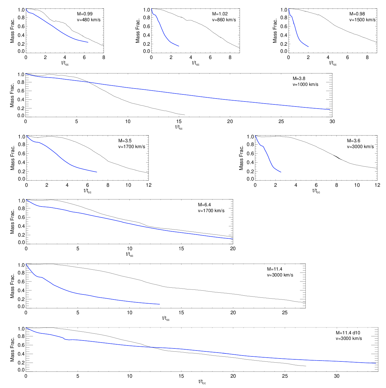
In Fig. 2, we show the mass retained by the cloud in each of these runs as a function of time in units of the cloud crushing time. More specifically, we plot , as defined in Paper I, the fraction of total mass above 1/3 the original cloud density. Unlike for the cases without thermal conduction, the choice of the threshold fraction (1/3) does not affect the results since evaporative compression causes a strong separation between the hot and cold phases. Fig. 2 captures the full evolution of the 9 cases including the high density model, which is at the bottom of the plot. The blue lines denote the results from the runs in this paper and the black lines are the results from the corresponding runs without thermal conduction from Paper I. It is clear from this figure that the KH instability does not play a significant role in the mass evolution. As found in Orlando (2004) the mass loss is dominated by evaporation off the cold cloud and not by hydrodynamic instabilities. Moreover, we see that in a few instances the lifetime of the clouds is longer when thermal conduction is switched on - contrary to what one might expect. The reasons lie in the balance of conduction and cooling as we will see below.
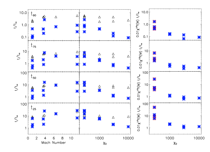
In Paper I, we were able to show that in the case without thermal conduction the lifetime of the cloud is almost completely dependent on Mach number. However, when we plot the disruption times of conducting clouds as a function of the Mach number, no clear trend emerges, as shown in the leftmost column of Fig. 3. On the other hand, when we plot the disruption times as a function of as in the central panels of this figure, we see that they scale roughly as .
In order to explain this dependence, we consider the balance between the internal energy that impinges on the cloud and the energy evaporated off it. The rate with which energy impinges on a cloud with cross-section is given by
| (9) |
where is the post-shock sound speed, is the velocity of the hot medium, is the density of the hot medium and is the ratio of specific heats. This heat goes into evaporating material off the cloud to a temperature beyond the peak of the cooling curve that allows it to decouple from the cloud. This temperature can be determined by measuring the mean temperature in the simulation within a density bracket of g cm-3. We find that this temperature, , is largely uniform across runs at K, a value just beyond the peak of , where radiative cooling becomes much less efficient. Note that the energy of the evaporating material is dominated by thermal energy, which is higher than its kinetic energy.
If we require this rate to balance the heating rate modulo a constant factor , we get
| (10) |
where , and the post-shock sound speed is given by
| (11) |
where 15 km/s is the sound speed inside the cloud (compare Eq. 17 and 50 in [6]; see also [31]). Note that is 1/4 of what it would be without conduction because of the modification of the shock jump conditions by thermal conduction, as described in Appendix A.
Dividing both sides of Eq. (10) by the initial mass of the cloud, , and expressing the mass loss rate in terms of the cloud crushing time, , we obtain
| (12) |
where
| (13) |
In the rightmost column of Fig. 3 we plot as given by Eq. (12), which shows most points reasonably level except for three outliers. Here we find that the value yields a good fit for most data points. If we assume that K, this implies that . Alternatively, if we want to keep , this would imply K.

The outliers are the runs for which radiative cooling in the evaporative flow is significant. Including optically thin cooling inside the blob, Eq. (10) becomes
| (14) |
where again is a constant factor. This can be rewritten as
| (15) |
which yields after expressing in terms of
| (16) |
where
Note that is purely a function of the initial column density of the cloud, We can solve Eq. (16), choosing the negative root in the quadratic formula as we are looking for solutions where . This gives
| (17) |
where . This implies that the timescale for evaporation, should be
| (18) |
In Fig. 4, is plotted as a function of the density ratio . Here we have taken and erg cm3/s appropriate for the the evaporating gas, which has been heated beyond the peak of the cooling function. Plugging in constants, one gets
| (19) |
When the cooling term is insignificant, then is small and that means that such that . When the cooling term is large, then . Interestingly, apart from the decreased temperature jump across the shock, none of this depends on the conduction law itself.
V. Morphology


To better illustrate the evolution of the clouds, in Figs. 5-7 we plot slices of the central density distribution at , , and . While the morphological evolution is relatively similar across the runs, the timescale of that evolution is not. At the clouds shrink and get denser as they are compressed by the evaporative flow. Interestingly, this compression is the highest in the cases with the lowest Mach number and lowest values of By setting the pressure behind the shock moving into the cloud due to evaporation equal to we can estimate the timescale for the cloud compression as
| (20) |
Again assuming that K this gives
| (21) |
This means that compression is most significant, i.e. that is smallest, when is small and the evaporation time is long compared to . Thus, for the lowest value cases at and the exterior pressure has managed to compress the entire cloud by , while for the cases with larger values the radius of the cloud is roughly halved. On the other hand, at higher and values, only the outer shell of the cloud is compressed and the density of the core of the cloud is lower.
At the clouds have a range of morphologies, depending on the ratio between and For the low and moderate and cases, the clouds have moved past the stage of initial compression and have begun to be stretched into filaments that are extremely narrow in the direction perpendicular to the flow, but extended in the streamwise direction. As in the case without conduction (see Paper I), the clouds are stretched mostly by the streamwise pressure gradient, rather than by shearing from the ambient medium. In these simulations, the density structure of the developing filament is complex: a lower density core is encased in a higher density shell, and the back of the cloud is flared due to the slightly lower pressure on the downstream side of the cloud. The flow around the filament is fairly laminar and there is little turbulent mixing. This can be quantified in terms of the dimensionless Peclet number, Pe, that is defined as the ratio between the advection rate and the diffusion rate, or , where is a typical length scale, is the velocity, is the density, is the specific heat at constant pressure and is the thermal conductivity. The flow outside of the very sharp boundary in density between the filament and the ambient flow has low Peclet numbers () which means that turbulent transport is negligible compared to the evaporative transport.
On the other hand, in the runs with larger and values, the clouds only reach the initial stage of compression at and they have not yet begun to be stretched at this time. In the fiducial run with , the cloud is still in the midst of its initial compression, but due to additional cooling, the run with ten times the initial density (and a larger ) is much further in its evolution. The difference between these two runs highlights the importance of column density in the evolution of the cloud, not only in determining the minimum cloud size as in eq. (8), but also in determining the rate of radiative cooling in the evaporating material for clouds above this threshold.
By even the fiducial run with relatively efficient cooling has produced a filament that has reached a length of at least twice the original cloud diameter. At each Mach number, the filaments flare at the downstream end, except in the cases in which the most compression times have passed and the interface between the cloud material and the ambient medium has become smoother. Furthermore, in the () and () cases, the leading edge of the filament has developed a bulbous morphology, trailed by a long cometary tail. Finally, at evaporative compression becomes significant in all cases, the filaments become very thin, and the clouds split into chains of smaller clumps that will soon be indistinguishable from the surrounding medium.
In Fig. 8 we show slices of the temperatures at for all the runs. The filamentary clouds are all cold with K material surrounded by a small corona that then blends into the hot ambient medium. As discussed in the Appendix, the temperature jumps seen in the runs occur just downstream from the shocks themselves, with important consequences for the conductive flux and the postshock temperature.
VI. Velocity Evolution
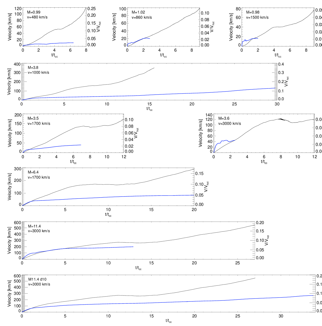
The impact of electron thermal conduction on cold cloud acceleration is even more dramatic than on the cloud disruption described above. In Fig. 9, we show the velocity evolution from our conduction runs, contrasted with the results without conduction from Paper I for the same choices of velocity and Mach number. Here we see that at early times the velocity of the clouds exceeds that in the runs without conduction, but soon afterwards the acceleration of the cold clouds becomes extremely inefficient. This is because in all our conducting runs, the cloud either evaporates within and is no longer distinguishable from the ambient medium or it compresses into a thin, long filament that has a small cross-section to the ambient wind. In the absence of conduction, the cloud velocity is set by the momentum imparted by the hot wind, which depends on the cross-section that the cloud presents to the hot flow. In Paper I, we estimated this velocity as
| (22) |
At early times, this estimate describes some of the runs with thermal conduction relatively accurately. However, from Fig. 9, it is apparent that in all cases the velocity attained by the cloud at late times, remains a small fraction of this value.
The large differences in the velocity evolution of the clouds are due to two important effects. The first is the compression of the clouds by the evaporating flow, which then causes it to present a very small cross-section to the wind after a time strongly limiting further acceleration. In addition, the evaporation of the cloud is biased in the downstream direction, yielding an extra increase in velocity due to the rocket effect, similar to what occurs in photoevaporative flows [47, 5, e.g,]. This is the cause of the increase in the cloud velocity at early times with respect to the results from Paper I.
Adding this additional source of acceleration to Eq. (22), rewriting as , and plugging in the compression time for , we get
| (23) |
where and are geometrical factors that quantify the efficiency of acceleration by the impinging flow and the evaporating material, respectively. In Fig. 10, we have plotted as given by Eq. (23) with and which gives a reasonable fit over our entire range of simulations. Note that in the cases in which cooling is negligible ( small and large), and the evaporation term is dominant, while in cases in which cooling is significant, is much longer and the shock term is most important.
In all cases, however, acceleration is inefficient with the cloud velocity reaching at most of at late times. Thus, in order for cold material entrained by a hot wind to reach velocities of the order of several hundred km/s as seen in some star-forming galaxies [55, 39] either other accelerating forces must be acting on the cloud or thermal conduction must be strongly suppressed by magnetic fields.

VII. Dependence on Numerical Resolution


Finally, we turn our attention to numerical convergence, which can particularly be a concern for problems that involve shearing instabilities and radiative cooling. Several authors recommend that the cloud radius be resolved with cells [35, 20]. Furthermore [74] pointed out that in order to capture the Rayleigh-Taylor and Kelvin-Helmholtz instabilities when radiative cooling is included, one must resolve the cooling length However, in our case, thermal conduction leads to a transition layer between the cold cloud and the hot, ambient medium which is thicker than and which damps these instabilities. Thus resolving is not expected to be necessary.
A second important length scale is the Field length, [17, 3], the maximum length scale across which thermal conduction can dominate over radiative cooling. For Spitzer conduction cm, which implies that in all our runs, in the ambient medium and inside the cloud . However, inside the cloud our setup does not allow any cooling because at temperatures K, cooling is switched off. As soon as material evaporates, the high pressure will not allow for fragmentation due to cooling, and thus resolving the Field length is not likely to be an issue.
To confirm these expectations, we have run our fiducial simulation with 4 (instead of 5) levels of refinement corresponding to a cell size of and also with a finer resolution than our fiducial run. In this case, the computing time requirements for a run with 6 levels of refinement were too high, so we settled for a run with a 50% higher peak resolution by increasing the number of blocks in each direction by 50%, yielding a cell size of . Since we enforce maximal resolution in and around the cold cloud, this minimum cell size was always maintained in the crucial parts of the simulation volume. This higher-resolution run took roughly 200,000 core hours on the Stampede supercomputer.
In Fig. 11, we have plotted the evolution of the cloud mass, , and cloud velocity as a function of time in these runs. The resulting curves for agree well, especially between the fiducial and the high-resolution run. Also the cloud velocities agree reasonably well between the fiducial and the high-resolution run. However, the low-resolution run with cm has a slightly higher mass and a resulting lower cloud velocity than the more highly resolved runs - a result of a non-negligible numerical viscosity. This implies that the spatial resolution chosen for our fiducial runs is sufficient and the scalings found in this paper do not depend on the grid size of the simulation.
VIII. Discussion and Summary
We have performed a suite of AMR hydrodynamical simulations of the evolution cold clouds in a hot wind, including both radiative cooling and electron thermal conduction. Observations of such K clouds are the primary probe of high-redshift galaxy outflows, and their evolution is highly dependent on the cloud column density, If the electron mean-free path is larger than the cloud radius, leading to runaway heating that quickly disrupts the cloud. On the other hand, if is above this threshold, cloud evolution is much more complex and gradual, and we have focused on this more interesting high-column density case in this study.
In this case, we have carried out nine different runs that span the range of conditions found in outflowing starburst galaxies, plus two more at varying spatial resolutions. As the equations that govern the evolution of the cloud are invariant under any transformation in which and these simulations also allow us to draw conclusions over a wide range of cloud properties. In all cases, the presence of electron thermal conduction drastically changes the morphological evolution, mass loss rate, and velocity evolution of the interacting clouds. While the outer layers of the clouds evaporate owing to thermal conduction, the cores are stretched into dense and cold filaments, as was also found by [44], [18], [49], and [27]. The simulations show how a conductive interface forms, leading to an increased density in the core that manages to radiate the energy conducted into the cloud, while stabilizing the cloud against hydrodynamical instabilities.
In Tab. 1, we list the times at which the masses of the clouds reach 90%, 75%, 50% and 25% of their original values, expressed in units of the cloud crushing time , with the initial density ratio between the cloud and the ambient medium, which is moving at a velocity . While in the absence of conduction the disruption time scales as , when thermal conduction is taken into account, the disruption times instead scale roughly as . We show that this dependence can be explained by considering the balance between the internal energy that impinges on a spherical cloud and the energy evaporated off the cloud. In particular, the heat impinging on the cloud goes into heating the material in the outer layers to a temperature beyond the peak of the cooling curve, which allows it to decouple from the cloud and evaporate.
In fact, accounting for radiative cooling in the evaporative flow yields an even better description of our results:
| (24) |
where is given by Eq. (19) and by Eq. (11). Thus, we can capture the combined effects of conduction and radiative cooling with a fairly simple analytic form, as shown in Fig. 4. Interestingly, this scaling does not depend on the form of the conduction law itself, apart from its role in affecting the temperature jump across the bow shock ahead of the cloud. In the downstream region the temperature is about 1/4 of the value that we would find for a shock in the absence of thermal conduction, and in the appendix of the paper we should how this value is determined by the electron sound speed and the fact that the temperature front moves out in front of the density discontinuity.
By considering the force of the evaporating flow on the cloud, we can also estimate the timescale for the cloud compression to be
| (25) |
implying that at the point at which the same fraction of the material is evaporated, compression will be most significant when the Mach number is small and when radiative losses in the evaporative flow are significant, extending These trends are in good correspondence to the morphologies observed in our simulations, which evolve from compression in an outer shell, to collapse to dense core, to stretching out into a dense filament that extends in the streamwise direction.
This evolution means that the cloud only presents an appreciable cross section to the wind for a time As a result the acceleration of the cold clouds by the ambient medium becomes inefficient, even though the presence of an evaporative flow has the potential to increase the velocity of the cloud due to the rocket effect. Estimating that the cloud acceleration occurs only on a timescale yields
| (26) |
where and are geometrical factors that quantify the efficiency of acceleration by the impinging flow and evaporated material. Again this is a good description of our numerical results tabulated in Tab. 1, with and giving the best match. We should add one caveat about our assumption to prevent cooling below temperatures of K while several observations of outflows do show a molecular component [21, e.g.]. With an HI photo-ionization cross-section of cm2, the cloud simulated in this paper would become optically thick with a neutral fraction of around 0.1%. Hence, for high enough column densities, shielding from the background might become important and lead to further cooling. This could result in longer cloud lifetimes and should be investigated using a full radiative transfer scheme.
Our simulations appear robust against changes in the resolution of the computational grid. In a convergence test, we found that the cloud mass does not change significantly between the and runs, and the velocity evolution does not change significantly between Finally, one can verify which regime of conduction applies to our setup. The energy flux that must pass through a radius around the cloud is and the density around the cloud is . This means that the ratio of the conductive flux into the cloud divided by the saturated flux is . Since the sound speed in the evaporating medium is approximately , this ratio is much less than 1, and the conductive flux is unsaturated. The condition for efficient conduction is when is sufficiently big for the saturated conductive heat flux to move faster than the energy flux of material flowing at its sound speed. Or in other words, energy needs to be able to move upstream in a flow for conductive evaporation to operate efficiently. If magnetic fields suppress this, the evaporation times found above could increase significantly.
If the suppression of conduction by magnetic fields is more modest, however, the mass and velocity scalings given above can be applied with significant confidence to future numerical and observational studies. In galaxy-scale simulations in which the evolution of individual clouds cannot be modeled with the required resolution directly, such clouds could be easily added as subgrid tracer particles, following our scalings for mass loss and cloud velocity. Observationally, our results can be used to help determine the possible origins of clouds given their velocities and positions with respect to the outflowing galaxy. A general conclusion in this case is that the acceleration of the cold clouds by the ambient medium is very inefficient in the presence of thermal conduction.
This means one of two things. Either magnetic fields must both strongly suppress conduction, or cold clouds with outflow velocities several 100 km/s cannot have been accelerated from purely by hot, outflowing material. The estimates of above suggest that conduction must be suppressed by a magnetic fields by a factor of at least to prevent cloud evaporation. In fact, at larger values the only place in which the conduction rate explicitly determines our results is in setting the value of the post-shock temperature, and decreasing conduction would increase this temperature not decrease it. If conduction indeed operates in this regime, then the most promising model for the origin of the cold clouds may be precipitation directly from the hot wind as a result of radiative cooling [69, 13, 61, 73, 40, 62, e.g.], rather than being swept up by the wind. On the other hand, in the case without conduction, [42] find that clouds with tangled internal magnetic fields are difficult to disrupt and the cloud fragments end up moving with the same speed as the external medium. Further investigation on the effects of the magnetic fields on the evolution of cold clouds in supersonic flows is clearly needed.
Appendix A: Shock Jump Conditions with Conduction
Here we examine how the temperature jump at the incoming shock is modified by saturated thermal conduction. Approximating the shock as planar and perpendicular to the direction of the flow, the equations of mass, momentum and energy conservation are
| (27) | |||||
| (28) | |||||
| (29) |
where in the last equation and we have neglected the upstream thermal pressure and its conductive flux. Comparing to the conduction law assumed in this paper, Eq. (5), and assuming , yields . Here the subscripts 1 and 2 denote upstream and downstream quantities, respectively. Radiative losses are not important for the shock structure in the conditions covered in this paper.


From mass and momentum conservation we can derive the jump condition for the velocity as
| (30) |
where is the isothermal Mach number. After a bit of algebra, we can also compute the ratio of velocities as
| (31) |
In the absence of conduction and in the limit of high , and . When the conductive term is nonzero, we can rewrite it as
| (32) |
Defining and Eq. (31) can then be rewritten as
| (33) |
We can solve this equation numerically as function of and When we look at the temperature across the bow shock in our simulation, we see that the temperature front is leading the density discontinuity and hence sits at a location where the density is 1/4 of the postshock density (see Fig. 12). This means that the conductive flux across the shock is set by the upstream density and the saturated flux is proportional to at a fixed temperature, i.e. , yielding an effective .
In addition, the solution to Eq. (33) only depends weakly on . Still, we can determine the effective Mach number at the shock by taking for the shock speed
| (34) | |||||
The Mach number of our shock is given by
| (35) |
Such that, for , the maximum of is .
References
- [1] Arrigoni Battaia, F., Hennawi, J. F., Prochaska, J. X., & Cantalupo, S. 2015, ApJ, 809, 163
- [2] Barai, P., Viel, M., Borgani, S., et al. 2013, MNRAS, 430, 3213
- [3] Begelman, M. C., & McKee, C. F. 1990, ApJ, 358, 375
- [4] Benson, A. J., Bower, R. G., Frenk, C. S., et al. 2003, ApJ, 599, 38
- [5] Bertoldi, F., & McKee, C. F. 1990, ApJ, 354, 529
- [6] Borkowski, K. J., Shull, J. M., & McKee, C. F. 1989, ApJ, 336, 979
- [7] Cen, R., & Chisari, N. E. 2011, ApJ, 731, 11
- [8] Chandrasekhar, S. 1961, Hydrodynamic and hydromagnetic stability, International Series of Monographs on Physics, Oxford: Clarendon
- [9] Cowie, L. L., & McKee, C. F. 1977, ApJ, 211, 135
- [10] Creasey, P., Theuns, T., & Bower, R. G. 2015, MNRAS, 446, 2125
- [11] Dalton, W. W., & Balbus, S. A. 1993, ApJ, 404, 625
- [12] Davé, R., Oppenheimer, B. D., & Finlator, K. 2011, MNRAS, 415, 11
- [13] Efstathiou, G. 2000, MNRAS, 317, 697
- [14] Erb, D. K., Quider, A. M., Henry, A. L., & Martin, C. L. 2012, ApJ, 759, 26
- [15] Ferland, G. J., Korista, K. T., Verner, D. A., et al. 1998, PASP, 110, 761
- [16] Ferrara, A., Scannapieco, E., & Bergeron, J. 2005, ApJ, 634, L37
- [17] Field, G. B. 1965, ApJ, 142, 531
- [18] Fragile, P. C., Murray, S. D., Anninos, P., & van Breugel, W. 2004, ApJ, 604, 74
- [19] Fryxell, B., Olson, K., Ricker, P., et al. 2000, ApJS, 131, 273
- [20] Fujita, A., Martin, C. L., Mac Low, M.-M., New, K. C. B., & Weaver, R. 2009, ApJ, 698, 693
- [21] Geach, J. E., Hickox, R. C., Diamond-Stanic, A. M., et al. 2014, Nature, 516, 68
- [22] Graham, R., & Langer, W. D. 1973, ApJ, 179, 469
- [23] Gray, W. J., & Scannapieco, E. 2010, ApJ, 718, 417
- [24] Gregori, G., Miniati, F., Ryu, D., & Jones, T. W. 1999, ApJ, 527, L113
- [25] Heckman, T. M. 2002, in Astronomical Society of the Pacific Conference Series, Vol. 254, Extragalactic Gas at Low Redshift, ed. J. S. Mulchaey & J. T. Stocke, 292
- [26] Heckman, T. M., Armus, L., & Miley, G. K. 1990, ApJS, 74, 833
- [27] Johansson, E. P. G., & Ziegler, U. 2013, ApJ, 766, 45
- [28] Kewley, L. J., & Ellison, S. L. 2008, ApJ, 681, 1183
- [29] Klein, R. I., McKee, C. F., & Colella, P. 1994, ApJ, 420, 213
- [30] Kornei, K. A., Shapley, A. E., Martin, C. L., et al. 2013, ApJ, 774, 50
- [31] Lacey, C. G. 1988, ApJ, 326, 769
- [32] Lee, D. 2013, Journal of Computational Physics, 243, 269
- [33] Li, S., Frank, A., & Blackman, E. G. 2013, ApJ, 774, 133
- [34] Mac Low, M.-M., McKee, C. F., Klein, R. I., Stone, J. M., & Norman, M. L. 1994, ApJ, 433, 757
- [35] Mac Low, M.-M., & Zahnle, K. 1994, ApJ, 434, L33
- [36] Mannucci, F., Cresci, G., Maiolino, R., Marconi, A., & Gnerucci, A. 2010, MNRAS, 408, 2115
- [37] Marcolini, A., Strickland, D. K., D’Ercole, A., Heckman, T. M., & Hoopes, C. G. 2005, MNRAS, 362, 626
- [38] Martin, C. L. 1999, ApJ, 513, 156
- [39] —. 2006, The Role of Galactic Winds in Galaxy Formation, ed. J. W. Mason, 337
- [40] Martin, C. L., Dijkstra, M., Henry, A., et al. 2015, ApJ, 803, 6
- [41] Martin, C. L., Scannapieco, E., Ellison, S. L., et al. 2010, ApJ, 721, 174
- [42] McCourt, M., O’Leary, R. M., Madigan, A.-M., & Quataert, E. 2015, MNRAS, 449, 2
- [43] McKee, C. F., & Begelman, M. C. 1990, ApJ, 358, 392
- [44] Mellema, G., Kurk, J. D., & Röttgering, H. J. A. 2002, A&A, 395, L13
- [45] Morel, J. E. 2000, J. Quant. Spec. Radiat. Transf., 65, 769
- [46] Nipoti, C., & Binney, J. 2007, MNRAS, 382, 1481
- [47] Oort, J. H., & Spitzer, Jr., L. 1955, ApJ, 121, 6
- [48] Orlando, S., Bocchino, F., Reale, F., Peres, G., & Pagano, P. 2008, ApJ, 678, 274
- [49] Orlando, S., Peres, G., Reale, F., et al. 2005, A&A, 444, 505
- [50] Pan, L., Desch, S. J., Scannapieco, E., & Timmes, F. X. 2012, ApJ, 756, 102
- [51] Peeples, M. S., Werk, J. K., Tumlinson, J., et al. 2014, ApJ, 786, 54
- [52] Pettini, M., Shapley, A. E., Steidel, C. C., et al. 2001, ApJ, 554, 981
- [53] Pichon, C., Scannapieco, E., Aracil, B., et al. 2003, ApJ, 597, L97
- [54] Pittard, J. M., & Parkin, E. R. 2015, ArXiv e-prints, arXiv:1510.05478
- [55] Rupke, D. S., Veilleux, S., & Sanders, D. B. 2005, ApJS, 160, 115
- [56] Scannapieco, E. 2013, ApJ, 763, L31
- [57] Scannapieco, E., & Brüggen, M. 2015, ApJ, 805, 158
- [58] Scannapieco, E., Ferrara, A., & Madau, P. 2002, ApJ, 574, 590
- [59] Schwartz, C. M., & Martin, C. L. 2004, ApJ, 610, 201
- [60] Shin, M.-S., Stone, J. M., & Snyder, G. F. 2008, ApJ, 680, 336
- [61] Silich, S., Tenorio-Tagle, G., & Muñoz-Tuñón, C. 2003, ApJ, 590, 791
- [62] Thompson, T. A., Quataert, E., Zhang, D., & Weinberg, D. H. 2016, MNRAS, 455, 1830
- [63] Tremonti, C. A., Heckman, T. M., Kauffmann, G., et al. 2004, ApJ, 613, 898
- [64] Turner, M. L., Schaye, J., Steidel, C. C., Rudie, G. C., & Strom, A. L. 2015, MNRAS, 450, 2067
- [65] Veilleux, S., Cecil, G., & Bland-Hawthorn, J. 2005, ARA&A, 43, 769
- [66] Veilleux, S., Teng, S. H., Rupke, D. S. N., Maiolino, R., & Sturm, E. 2014, ApJ, 790, 116
- [67] Vieser, W., & Hensler, G. 2007a, A&A, 475, 251
- [68] —. 2007b, A&A, 472, 141
- [69] Wang, B. 1995, ApJ, 444, 590
- [70] Wang, J., Nardini, E., Fabbiano, G., et al. 2014, ApJ, 781, 55
- [71] Weiner, B. J., Coil, A. L., Prochaska, J. X., et al. 2009, ApJ, 692, 187
- [72] Wiersma, R. P. C., Schaye, J., & Smith, B. D. 2009, MNRAS, 393, 99
- [73] Wünsch, R., Silich, S., Palouš, J., Tenorio-Tagle, G., & Muñoz-Tuñón, C. 2011, ApJ, 740, 75
- [74] Yirak, K., Frank, A., & Cunningham, A. J. 2010, ApJ, 722, 412
- [75] Zhang, D., Thompson, T. A., Quataert, E., & Murray, N. 2015, ArXiv e-prints, arXiv:1507.01951