Enhanced violation of the Collins-Gisin-Linden-Massar-Popescu inequality
with optimized time-bin-entangled ququarts
Abstract
High-dimensional quantum entanglement is drawing attention because it enables us to perform quantum information tasks that are robust against noises. To test the nonlocality of entangled qudits, the Collins-Gisin-Linden-Massar-Popescu (CGLMP) inequality has been proposed and demonstrated using qudits based on orbital angular momentum, time-energy uncertainty, and frequency bins. Here, we report the generation and observation of time-bin entangled ququarts. We implemented a measurement for the CGLMP inequality test using cascaded delay Mach-Zehnder interferometers fabricated by using planar lightwave circuit technology, with which we achieved a precise and stable measurement for time-bin-entangled ququarts. In addition, we generated an optimized entangled state by modulating the pump pulse intensities, with which we can observe the theoretical maximum violation for the CGLMP inequality test. As a result, we successfully observed a Bell-type parameter violating the CGLMP inequality for the maximally entangled state and an enhanced Bell-type parameter for the optimized entangled state.
pacs
Valid PACS appear hereI Introduction
Quantum entanglement has a strange non-local characteristic unique to quantum particles, known as the Einstein-Podolsky-Rosen paradox [1]. Ever since the first reports of the violation of Bell’s inequality [2, 3], the non-locality of quantum entanglement has been widely confirmed, and subsequent efforts to overcome the loopholes have been reported [4, 5, 6, 7, 8, 9]. Now quantum entanglement has been utilized for many quantum communication tasks such as quantum key distribution (QKD) [10], quantum teleportation [11], and quantum repeaters [12, 13]. Recently, entangled qudits, or high-dimensional entanglement, have been attracting attention, because they enable us to perform robust quantum information tasks. For example, it has been theoretically shown [14, 15] and experimentally demonstrated [16, 17, 18] that we can improve the error rate tolerance for QKD. Furthermore, the amount of information per photon can be increased [18]. In addition, we can use the entangled qudits to relax the condition for closing the detection loophole in Bell’s inequality tests [19].
To test the nonlocality of the entangled qudits, Collins, Gisin, Linden, Massar, and Popescu (CGLMP) proposed a Bell-type inequality[20]. A unique characteristic of the CGLMP inequality is that non-maximally entangled states give the theoretical maximum violation of the inequality for , where is a Hilbert space dimension of a particle [21]. So far, CGLMP inequality tests have been performed by using qudits based on orbital angular momentum (OAM) [22, 21], time-energy uncertainty [23, 24], and frequency-bins [25, 26]. Among these, OAM-based entangled qudits have been intensively studied, and even a dimensional entanglement has been demonstrated [27]. Despite their advantage for scalability, OAM-based qudits are not suitable for the fiber transmission required for long-distance terrestrial QKD because of the spatial mode dispersion in fiber. Time-energy entangled photon pairs are promising candidates for fiber transmission. However, with time-energy entanglement, it is difficult to generate the optimized entangled state for obtaining the maximum violation of the CGLMP inequality. Bernhard et al. [26] attempted to generate optimized frequency-bin-entangled qudits with spatial light modulators (SLMs). They successfully observed violations of the CGLMP inequality; however, no significant difference between the maximally entangled qudits and the optimized entangled qudits was observed. In addition, the optimization using SLMs causes excess loss, which results in a lower coincidence rate in the CGLMP measurement.
Here, we report the generation and observation of time-bin-entangled ququarts, or four-dimensional entangled photon pairs. We used cascaded delay Mach-Zehnder interferometers (MZIs) [23] to implement a measurement for the CGLMP inequality test for the time-bin-entangled ququarts. An advantage of cascaded delay MZIs is that they require fewer optical passes than multi-arm interferometers [24]. A drawback of this implementation is that it introduces more loss than the multi-arm interferometers. Using cascaded delay MZIs made with planar lightwave circuit technology (PLC), we observed clear two-photon interferences and a direct violation of the CGLMP inequality. Furthermore, we generated an optimized entangled state that enabled the maximum violation of the CGLMP inequality. We were able to modulate probability amplitudes of the time-bin-entangled ququarts to obtain the optimized entangled state simply by modulating pump pulse intensities. Consequently, we observed an enhanced violation of the CGLMP inequality by 39 standard deviations with the optimized entangled state.
II The CGLMP inequality and optimized entangled state
The CGLMP inequality [20] is a natural extension of the Clauser-Horne-Shimony-Holt (CHSH) inequality [28]. In the CHSH inequality, we quantify the correlation between two photons by values according to the results measured on the each side of the receivers, Alice and Bob. With a high-dimensional system, however, there are more orthogonal states than 2, and we thus need more values corresponding to these states. For this purpose, the CGLMP inequality has a Bell-type parameter, which is given by
| (1) |
where is the dimension and and are Alice and Bob’s measurement outcomes when they select the bases , , respectively. is a conditional probability that is equal to modulo when measurement bases are set at and , where , , , , and . In the local hidden variable theory, satisfies the following inequality as with the CHSH inequality [20]:
| (2) |
However, this inequality is violated using quantum entanglement; therefore, the violation of the CGLMP inequality is good evidence of a high-dimensional entanglement.
For this test, one can use the maximally entangled state, which is given by
| (3) |
where and are states that photons for Alice and Bob exist in the -th time slot, respectively. Using the maximally entangled state, we can observe the violation of the CGLMP inequality. In the two-dimensional system, the violation obtained with the maximally entangled state is the theoretical maximum violation for any state. In a high-dimensional system, however, non-maximally entangled states can give the maximum violation. In [21], Dada et al. derived the optimized entangled state to obtain the maximum violation. The optimized entangled state is an eigenstate of an operator representing the measurement of . For example, the optimized entangled ququarts are given by
| (4) |
where is an amplitude modulation factor and is a short form of for simplicity. Table 1 shows the theoretical maximum values for the maximally entangled states and the optimized entangled states for various values derived as in [21]. The theoretical maximum for the optimized entangled state, , is larger than the theoretical maximum for the maximally entangled state, .
| for | for | |
|---|---|---|
| 2 | 2.8284 | 2.8284 |
| 3 | 2.8729 | 2.9149 |
| 4 | 2.8962 | 2.9727 |
| ⋮ | ⋮ | ⋮ |
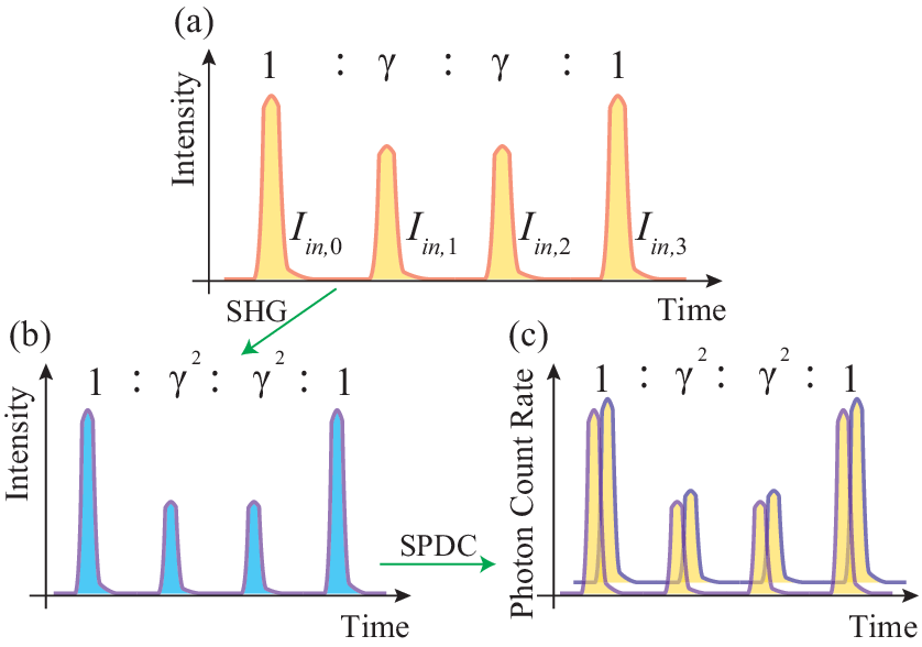
In our experiment, we generate the time-bin-entangled state by utilizing spontaneous parametric down conversion (SPDC) pumped by pulses generated via second harmonic generation (SHG). Through the SHG process, the field amplitude of generated light is proportional to the intensity of input light . The probability amplitude of a photon pair state generated via SPDC satisfies . We used these relations to generate the optimized time-bin-entangled ququarts. Figure 1 shows the concept of the optimized time-bin-entangled ququarts generation. We modulate a classical lightwave into four-sequential pulses so that the intensities of the four-sequential pulses satisfy the following equation: , where is the intensity of light in the -th time slot. Then, the generated time-bin-entangled state satisfies
| (5) |
Thus, with the time-bin-entangled qudits, we can obtain the optimized entangled state simply by modulating the amplitudes of the pump pulses without excess loss.
III Measurement for the CGLMP inequality

In the CGLMP inequality test, we perform a measurement projecting onto the Fourier transform basis. The Fourier transform basis is composed of sates , which are given by
| (6) |
Phase in Eq. (6) takes
| (7) |
where , , , , and is an integer that denotes the measurement outcomes. We use the cascaded delay MZIs to perform this measurement. Note that a similar scheme based on cascaded MZIs was proposed in [23]. However, a measurement corresponding to Eq. (6) has not been implemented using the scheme yet. Figure 2 shows the concept of the measurement using the cascaded MZIs for four dimensions. The first MZI has a time delay and a phase shift , where denotes the temporal interval between time bins and the phase difference between the short and long arms. On the other hand, the second MZI has a time delay and a phase shift .
Here, we define a generalized measurement operator , which expresses the function of the first MZI at port in Fig. 2 as
| (8) |
A complementary operator corresponding to the function of the first MZI at port is defined so as to satisfy , where is the identity operator for the input state space. Similarly, we define another generalized measurement operator for the second MZI at port as
| (9) |
where is defined so as to satisfy . Therefore, the function of the cascaded MZIs at port is given by . We postselect a state in which all the input time slots overlap in order to obtain the probability corresponding to the projection onto Eq. (6). The postselection corresponds to the projection onto at port . Thus, the whole measurement operator for our measurement setup with is given by
| (10) | |||||
If we have a density operator of input time-bin state , the probability of finding a photon in the fourth time slot at port is given by . Thus, we can obtain the probability of projecting the input state onto Eq. (6) by extracting photon detection events in the fourth time slot.
IV Experimental setup
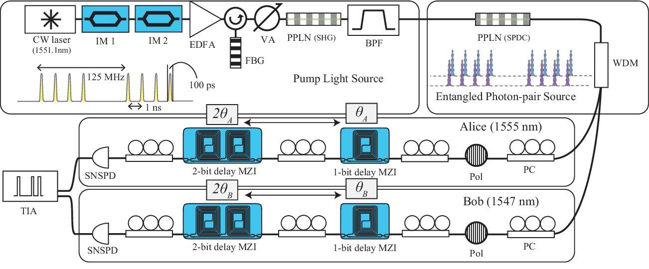
Figure 3 shows the experimental setup. First, we generate four sequential pulses by modulating a CW laser light with a 1551.1-nm wavelength. The temporal interval, pulse duration, and repetition frequency are 1 ns, 100 ps, and 125 MHz, respectively. IM 1 is used only when we generate the optimized entangled state, and IM 2 is used to shape the time slots. We then amplify the pulse train using an EDFA and adjust the average power of the pulse train with a VA. These pulses are launched into a PPLN waveguide, where 780-nm pump pulses are generated via SHG. The 780-nm pump pulses are input into another PPLN waveguide so that we can generate time-bin-entangled ququarts whose state is expressed as Eq. (3) or (4) through SPDC. The generated photon pairs are separated into channels A and B by wavelengths using a WDM. The wavelengths of channels A and B are 1555 and 1547 nm, respectively, both with a 100-GHz bandwidth. Photons A and B are sent to Alice and Bob, where they perform the measurement denoted by Eq. (6) using the cascaded MZIs, whose output ports are connected to SNSPDs. Here, we employ 1- and 2-ns delay MZIs, which we call 1- and 2-bit delay MZIs, respectively. These MZIs are fabricated using PLC and are thus very stable [29, 30]. The phase shifts of each MZI are precisely controlled by means of the thermooptic effect caused by electrical heaters attached to the waveguides. The phase shifts of 1- and 2-bit delay MZIs are synchronized so that we can perform the measurement expressed as Eq. (6). Polarization controllers are placed in front of each MZI to operate them for one polarization. The detection event signals from the SNSPDs are input into a TIA, where coincidence analysis is performed. The detection efficiencies of the SNSPDs for Alice and Bob are 19 and 17 %, respectively, both with a -cps dark count rate.
V Results
V.1 Maximally entangled state

We first generated a maximally entangled state. Figure 4 shows the result when Alice swept her phase of the cascaded MZIs, , from to while Bob set his phase, , at or . Circles and triangles are measured coincidence counts for and , respectively, and solid and dotted lines show the fitted curves obtained with the Levenberg-Marquardt algorithm. The average photon pair number per ququart was set at 0.01, and measurement time for each phase combination was 90 sec. Note that throughout this work we did not subtract any noise counts, including accidental coincidence counts due to detector dark counts or multi-photon emissions. We observed clear coincidence fringes, which are different from the cosine-curve fringes obtained with entangled qubits and unique to entangled ququarts. In addition, we observed a clear correlation for two non-orthogonal bases at Bob’s measurement, which indicated the existence of a non-classical correlation between ququarts. For an ideal maximally entangled state, the coincidence count probability is given by
| (11) | |||||
Therefore, the measured coincidence count in the experiment can be fitted with
| (12) |
where is the difference between the maximum and the minimum values of , ans are fitting parameters. The visibility of the coincidence fringe is given by
| (13) |
From the fitted curves, we obtained of and for and , respectively. If we assume symmetric noise, the depolarized mixed state is given by
| (14) |
where is a mixing parameter and is the identity operator for the entangled ququarts space. From this assumption, the visibility is related to with the following equation:
| (15) |
If , the state can violate the CGLMP inequality. Thus a visibility of , obtained by substituting into Eq. (15) , is a critical limit for a coincidence fringe of the maximally entangled state to violate the CGLMP inequality. Our results— and —are obviously larger than .

We also performed an measurement for the CGLMP inequality test by performing the coincidence measurements for 64 combinations of and . Figure 5 shows coincidence measurements when and were set at 41 and 8 points in their phase range and , respectively. The average photon pair number per ququart was set at 0.01, and the measurement time for each phase combination was 120 sec. The coincidence counts for the maximally entangled state in the measurement for the CGLMP inequality test are shown in Table 2 in Appendix A. With those data, we obtained of where the error was estimated by assuming Poisson statistics. This value violates the CGLMP inequality by 31 standard deviations.
V.2 Optimized entangled state
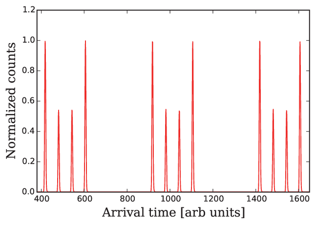
To generate the optimized entangled state, we modulated the CW light with IM 1 in Fig. 3 so that the generated time-bin-entangled ququarts satisfied the condition in Eq. (5). IM 2 was used to shape the light into four sequential pulses. Figure 6 shows a histogram of the photon detection at channel A measured after the WDM filter. The four peaks correspond to the probabilities of finding a photon in time slots 0, 1, 2, and 3, respectively. From the histogram, we confirmed the experimental amplitude modulation factor , which was very close to the target value (0.739).

We performed a coincidence fringe measurement. Triangles in Fig. 7 show the normalized coincidence as a function of when was set at 0. The average photon pair number per ququart was set at 0.02, and the measurement time for each phase setup combination was 60 sec. The result for the maximally entangled state when Bob set his phase at 0 is also plotted for comparison (denoted by circles). The smaller two peaks are enhanced compared with those for the maximally entangled state, which is a feature of the coincidence fringe shape for the optimized entangled state. For an ideal optimized entangled state, the coincidence count probability is given by
| (16) |
Therefore, the measured coincidence count in the experiment can be fitted by
| (17) |
where
| (18) |
and the visibility is given by Eq. (13). From the fitted curves, we obtain and for and , respectively. Estimating the critical limit with a similar procedure used for the maximally entangled state, we obtain the limit of the visibility . Thus, the visibilities obtained in our experiment were larger than the critical limit for violating the CGLMP inequality.
Finally, we performed an measurement for the CGLMP inequality test with the optimized entangled state. The average photon pair number per ququart was set at 0.01, and the measurement time for each phase setup combination was 120 sec. As a result, we obtained of , which violated the CGLMP inequality by 39 standard deviations (the coincidence count data are shown in Table 3 in Appendix A). Thus, we successfully confirmed that the use of the optimized entangled state leads to clear enhancements of both the value of and the violation of the classical limit compared with those obtained with the maximally entangled state.
Unfortunately, there were discrepancies between our results and the theoretical maximum in Table 1. The effects of accidental coincidences caused by the detector dark counts were negligibly small. The effect caused by multi-photon emission would be a main source of the deviation (see Appendix B). Another source of the deviation was phase drift due to variations in the CW laser frequency and MZIs settings during the long measurements required for the coincidence measurements with many phase combinations. In addition, the loss difference between the long and short arms of the MZIs may have resulted in the non-ideal measurements for the ququarts. The accumulation of these experimental defects caused the deviations of the measured values from the theoretical ones.
VI Conclusion
We have described a CGLMP inequality test using optimized time-bin ququarts. We generated the optimized entangled ququarts by modulating the pump pulse amplitudes and implemented the measurement for the CGLMP inequality test with cascaded MZIs. We observed Bell-type parameters and for the maximally entangled state and the optimized entangled state, respectively. As a result, we observed the enhancement of both the value of and the violation of the CGLMP inequality with the optimized entangled ququarts. We hope that our result will lead to advanced quantum communications systems such as high-dimensional robust QKD systems.
Acknowledgements.
We thank K. Inoue, K. Igarashi, N. Matsuda, and F. Morikoshi for fruitful discussions.Appendix A Coincidence count data for the measurements
Here, we show the coincidence count results for the measurements. Tables 2 and 3 show the raw coincidence count data for the maximally entangled state and the optimized entangled state, respectively. The details of the measurement conditions are described in Sec. V. From these results, we calculated the coincidence probabilities and obtained by substituting them into Eq. (1).
| Bob | ||||||||||
|---|---|---|---|---|---|---|---|---|---|---|
| Basis 0 | Basis 1 | |||||||||
| 0 | 605 | 72 | 34 | 49 | 493 | 36 | 37 | 67 | ||
| Basis | 46 | 453 | 74 | 17 | 62 | 545 | 31 | 38 | ||
| 0 | 29 | 40 | 508 | 85 | 30 | 45 | 555 | 27 | ||
| Alice | 102 | 32 | 33 | 535 | 26 | 26 | 48 | 671 | ||
| 102 | 529 | 40 | 47 | 515 | 94 | 23 | 53 | |||
| Basis | 30 | 28 | 473 | 28 | 22 | 445 | 92 | 24 | ||
| 1 | 47 | 15 | 97 | 581 | 25 | 28 | 581 | 98 | ||
| 611 | 22 | 18 | 48 | 67 | 27 | 34 | 600 | |||
| Bob | ||||||||||
|---|---|---|---|---|---|---|---|---|---|---|
| Basis 0 | Basis 1 | |||||||||
| 0 | 544 | 38 | 21 | 60 | 517 | 54 | 33 | 30 | ||
| Basis | 57 | 426 | 46 | 24 | 24 | 458 | 47 | 53 | ||
| 0 | 29 | 63 | 470 | 25 | 20 | 26 | 453 | 53 | ||
| Alice | 30 | 49 | 63 | 408 | 57 | 43 | 21 | 445 | ||
| 57 | 462 | 64 | 42 | 517 | 40 | 18 | 84 | |||
| Basis | 52 | 29 | 422 | 35 | 57 | 398 | 44 | 20 | ||
| 1 | 70 | 28 | 51 | 439 | 56 | 80 | 430 | 31 | ||
| 459 | 55 | 48 | 30 | 44 | 40 | 71 | 408 | |||
Appendix B Effect caused by multi-photon emission
Here, we estimate the degradation of the visibility and caused by the multi-photon emission. In our experiment, the coherence time of a single photon (10 ps) was much smaller than the pump pulse duration. Thus, the multiple photons can be approximated to distinguishable photons. It is known that the number of such a distinguishable photon pair generated via SPDC follows a Poisson distribution [31]. Therefore, we can estimate the coincidence probability as follows. From the Poisson statistics, the probability of generating photon pairs is given by
| (19) |
where is a average number of photon pairs. When we generate photon pairs (), the probability of losing photons at Alice’s side because of the medium loss, , is given by
| (20) |
where is a transmittance including detector efficiency. When Alice receives photons, the probability of Alice detecting photons in her measurement setup, , is given by
| (21) |
where
| (22) |
and are a density operator of a single photon pair and a generalized measurement operator for Alice’s measurement setup, respectively. For example, and for our coincidence measurement with the optimized entangled state.
Here, we define probabilities , , and as follows.
| (23) | |||||
| (24) | |||||
| (25) | |||||
| (26) |
where is a generalized measurement operator for Bob. The pairs of photons detected by Alice are detected by Bob with a probability . The pairs of photons that are not lost in transmission and not detected in Alice’s measurement setup are detected by Bob with a probability . The pairs of photons lost in transmission are detected by Bob with a probability . Our SNSPD cannot resolve the number of the detected photons, so the coincidence probability on the above conditions, , is given by
| (27) |
By utilizing Eqs. (19) – (21) and (27), the coincidence probability is given by
| (28) |
By calculating the summation in Eq. (28), we obtain
| (29) |
When , Eq. (29) is approximated as
| (30) |
For example, when we use the optimized entangled ququarts and cascaded MZIs, probabilities , , and are given by
| (31) | |||||
| (32) |
By substituting these probabilities into Eq. (30) and using the definition of visibility, we obtain the visibility as
| (33) |
We combine Eq. (33) and the visibility for the optimized entangled ququarts as a function of the mixing parameter as Eq. (15), and is given by
| (34) |
We obtain for . This predicts of , which is close to our experimental result of .
References
- [1] A. Einstein, B. Podolsky, and N. Rosen, Can Quantum-Mechanical Description of Physical Reality Be Considered Complete? Physical Review 47, 777 (1935).
- [2] S. J. Freedman and J. F. Clauser, Experimental Test of Local Hidden-Variable Theories, Physical Review Letters 28, 938 (1972).
- [3] A. Aspect, P. Grangier, and G. Roger, Experimental tests of realistic local theories via Bell’s theorem, Physical Review Letters 47, 460 (1981).
- [4] M. Ansmann, H. Wang, R. C. Bialczak, M. Hofheinz, E. Lucero, M. Neeley, A. D. O’Connell, D. Sank, M. Weides, J. Wenner, A. N. Cleland, and J. M. Martinis, Violation of Bell’s inequality in Josephson phase qubits, Nature 461, 504 (2009).
- [5] M. Giustina, A. Mech, S. Ramelow, B. Wittmann, J. Kofler, J. Beyer, A. Lita, B. Calkins, T. Gerrits, S. W. Nam, R. Ursin, and A. Zeilinger, Bell violation using entangled photons without the fair-sampling assumption, Nature 497, 227 (2013).
- [6] B. G. Christensen, K. T. McCusker, J. B. Altepeter, B. Calkins, T. Gerrits, A. E. Lita, A. Miller, L. K. Shalm, Y. Zhang, S. W. Nam, N. Brunner, C. C. W. Lim, N. Gisin, and P. G. Kwiat, Detection-Loophole-Free Test of Quantum Nonlocality, and Applications, Physical Review Letters 111, 130406 (2013).
- [7] B. Hensen, H. Bernien, A. E. Dréau, A. Reiserer, N. Kalb, M. S. Blok, J. Ruitenberg, R. F. L. Vermeulen, R. N. Schouten, C. Abellán, W. Amaya, V. Pruneri, M. W. Mitchell, M. Markham, D. J. Twitchen, D. Elkouss, S. Wehner, T. H. Taminiau, and R. Hanson, Loophole-free Bell inequality violation using electron spins separated by 1.3 kilometres, Nature 526, 682 (2015).
- [8] M. Giustina, M. A. M. Versteegh, S. Wengerowsky, J. Handsteiner, A. Hochrainer, K. Phelan, F. Steinlechner, J. Kofler, J.-Å. Larsson, C. Abellán, W. Amaya, V. Pruneri, M. W. Mitchell, J. Beyer, T. Gerrits, A. E. Lita, L. K. Shalm, S. W. Nam, T. Scheidl, R. Ursin, B. Wittmann, and A. Zeilinger, Significant-Loophole-Free Test of Bell’s Theorem with Entangled Photons, Physical Review Letters 115, 250401 (2015).
- [9] L. K. Shalm, E. Meyer-Scott, B. G. Christensen, P. Bierhorst, M. A. Wayne, M. J. Stevens, T. Gerrits, S. Glancy, D. R. Hamel, M. S. Allman, K. J. Coakley, S. D. Dyer, C. Hodge, A. E. Lita, V. B. Verma, C. Lambrocco, E. Tortorici, A. L. Migdall, Y. Zhang, D. R. Kumor, W. H. Farr, F. Marsili, M. D. Shaw, J. A. Stern, C. Abellán, W. Amaya, V. Pruneri, T. Jennewein, M. W. Mitchell, P. G. Kwiat, J. C. Bienfang, R. P. Mirin, E. Knill, and S. W. Nam, Strong Loophole-Free Test of Local Realism, Physical Review Letters 115, 250402 (2015).
- [10] A. K. Ekert, Quantum Cryptography Based on Bell’s Theorem, Physical Review Letters 67, 661 (1991).
- [11] C. H. Bennett, G. Brassard, C. Crépeau, R. Jozsa, A. Peres, and W. K. Wootters, Teleporting an unknown quantum state via dual classical and Einstein-Podolsky-Rosen channels, Physical Review Letters 70, 1895 (1993).
- [12] N. Sangouard, C. Simon, H. De Riedmatten, and N. Gisin, Quantum repeaters based on atomic ensembles and linear optics, Reviews of Modern Physics 83, 33 (2011).
- [13] K. Azuma, K. Tamaki, and H.-K. Lo, All-photonic quantum repeaters, Nature Communications 6, 6787 (2015).
- [14] N. J. Cerf, M. Bourennane, A. Karlsson, and N. Gisin, Security of Quantum Key Distribution Using d-Level Systems, Physical Review Letters 88, 127902 (2002).
- [15] L. Sheridan and V. Scarani, Security proof for quantum key distribution using qudit systems, Physical Review A 82, 030301 (2010).
- [16] S. Gröblacher, T. Jennewein, A. Vaziri, G. Weihs, and A. Zeilinger, Experimental quantum cryptography with qutrits, New Journal of Physics 8, 75 (2006).
- [17] M. Mafu, A. Dudley, S. Goyal, D. Giovannini, M. McLaren, M. J. Padgett, T. Konrad, F. Petruccione, N. Lütkenhaus, and A. Forbes, Higher-dimensional orbital-angular-momentum-based quantum key distribution with mutually unbiased bases, Physical Review A 88, 032305 (2013).
- [18] T. Zhong, H. Zhou, R. D. Horansky, C. Lee, V. B. Verma, A. E. Lita, A. Restelli, J. C. Bienfang, R. P. Mirin, T. Gerrits, S. W. Nam, F. Marsili, M. D. Shaw, Z. Zhang, L. Wang, D. Englund, G. W. Wornell, J. H. Shapiro, and F. N. C. Wong, Photon-efficient quantum key distribution using time-energy entanglement with high-dimensional encoding, New Journal of Physics 17, 022002 (2015).
- [19] T. Vértesi, S. Pironio, and N. Brunner, Closing the Detection Loophole in Bell Experiments Using Qudits, Physical Review Letters 104, 060401 (2010).
- [20] D. Collins, N. Gisin, N. Linden, S. Massar, and S. Popescu, Bell Inequalities for Arbitrarily High-Dimensional Systems, Physical Review Letters 88, 040404 (2002).
- [21] A. C. Dada, J. Leach, G. S. Buller, M. J. Padgett, and E. Andersson, Experimental high-dimensional two-photon entanglement and violations of generalized Bell inequalities, Nature Physics 7, 677 (2011).
- [22] A. Vaziri, G. Weihs, and A. Zeilinger, Experimental two-photon, three-dimensional entanglement for quantum communication. Physical Review Letters 89, 240401 (2002).
- [23] D. Richart, Y. Fischer, and H. Weinfurter, Experimental implementation of higher dimensional time-energy entanglement, Applied Physics B 106, 543 (2012).
- [24] R. T. Thew, A. Acín, H. Zbinden, and N. Gisin, Bell-Type Test of Energy-Time Entangled Qutrits, Physical Review Letters 93, 010503 (2004).
- [25] B. Bessire, C. Bernhard, T. Feurer, and A. Stefanov, Versatile shaper-assisted discretization of energy-time entangled photons, New Journal of Physics 16, 033017 (2014).
- [26] C. Bernhard, B. Bessire, T. Feurer, and A. Stefanov, Shaping frequency-entangled qudits, Physical Review A 88, 032322 (2013).
- [27] M. Krenn, M. Huber, R. Fickler, R. Lapkiewicz, S. Ramelow, and A. Zeilinger, Generation and confirmation of a (100 100)-dimensional entangled quantum system, Proceedings of the National Academy of Sciences 111, 6243 (2014).
- [28] J. F. Clauser, M. A. Horne, A. Shimony, and R. A. Holt, Proposed Experiment to Test Local Hidden-Variable Theories, Physical Review Letters 23, 880 (1969).
- [29] H. Takesue and K. Inoue, Generation of 1.5-m band time-bin entanglement using spontaneous fiber four-wave mixing and planar light-wave circuit interferometers, Physical Review A 72, 041804 (2005).
- [30] T. Honjo, K. Inoue, and H. Takahashi, Differential-phase-shift quantum key distribution experiment with a planar light-wave circuit Mach-Zehnder interferometer, Optics Letters 29, 2797 (2004).
- [31] H. Takesue and K. Shimizu, Effects of multiple pairs on visibility measurements of entangled photons generated by spontaneous parametric processes, Optics Communications 283, 276 (2010).