Direct Arbitrary-Lagrangian-Eulerian finite volume schemes on moving nonconforming unstructured meshes
Abstract
In this paper, we present a novel second-order accurate Arbitrary-Lagrangian-Eulerian (ALE) finite volume scheme on moving nonconforming polygonal grids, in order to avoid the typical mesh distortion caused by shear flows in Lagrangian-type methods. In our new approach the nonconforming element interfaces are not defined by the user, but they are automatically detected by the algorithm if the tangential velocity difference across an element interface is sufficiently large. The grid nodes that are sufficiently far away from a shear wave are moved with a standard node solver, while at the interface we insert a new set of nodes that can slide along the interface in a nonconforming manner. In this way, the elements on both sides of the shear wave can move with a different velocity, without producing highly distorted elements.
The core of the proposed method is the use of a space-time conservation formulation in the construction of the final finite volume scheme, which completely avoids the need of an additional remapping stage, hence the new method is a so-called direct ALE scheme. For this purpose, the governing PDE system is rewritten at the aid of the space-time divergence operator and then a fully discrete one-step discretization is obtained by integrating over a set of closed space-time control volumes. The nonconforming sliding of nodes along an edge requires the insertion or the deletion of nodes and edges, and in particular the space-time faces of an element can be shared between more than two cells.
Due to the space-time conservation formulation, the geometric conservation law (GCL) is automatically satisfied by construction, even on moving nonconforming meshes. Moreover, the mesh quality remains high and, as a direct consequence, also the time step remains almost constant in time, even for highly sheared vortex flows. In this paper we focus mainly on logically straight slip-line interfaces, but we show also first results for general slide lines that are not logically straight. Second order of accuracy in space and time is obtained by using a MUSCL-Hancock strategy, together with a Barth and Jespersen slope limiter.
The accuracy of the new scheme has been further improved by incorporating a special well balancing technique that is able to maintain particular stationary solutions of the governing PDE system up to machine precision. In particular, we consider steady vortex solutions of the shallow water equations, where the pressure gradient is in equilibrium with the centrifugal forces.
A large set of different numerical tests has been carried out in order to check the accuracy and the robustness of the new method for both smooth and discontinuous problems. In particular we have compared the results for a steady vortex in equilibrium solved with a standard conforming ALE method (without any rezoning technique) and with our new nonconforming ALE scheme, to show that the new nonconforming scheme is able to avoid mesh distortion in vortex flows even after very long simulation times.
Keywords:
moving nonconforming unstructured meshes, slide lines in direct Arbitrary-Lagrangian-Eulerian (ALE) methods for shear flows, cell-centered Godunov-type finite volume methods, shallow water equations in Cartesian and cylindrical coordinates, hyperbolic conservation laws, well balanced methods.1 Introduction
Arbitrary-Lagrangian-Eulerian (ALE) finite volume schemes are characterized by a moving computational mesh: at each time step the new position of all the nodes has to be recomputed according to a prescribed mesh velocity, which generally is chosen as close as possible to the local fluid velocity (as it is in the purely Lagrangian framework), but it can also be set to zero (to reproduce the Eulerian case), or it can be chosen arbitrarily. The aim of these methods is to reduce the numerical dissipation errors due to the convective terms, hence to capture contact discontinuities sharply and to precisely identify and track material interfaces. For these reasons already in the 1950’s John von Neumann and Richtmyer were working on Lagrangian schemes [68] for one-dimensional flows, and Wilkins proposed a two-dimensional extension in 1964, see [69]. Since the fluid velocity is required at each node and at each time step, a natural approach is a staggered discretization, where the momentum is defined at the grid vertices and all the other flow variables are defined at the cell center. Despite some drawbacks of the initial version of staggered Lagrangian schemes, which was not conservative and which produced some spurious modes in the numerical solution, it was widely used in the last forty years and many improvements have been made in the meantime; for further details one can refer to the papers of Caramana and Shashkov [21, 22] and of Loubère at al. [53, 54]. Moreover, examples on general polygonal grids have been presented in [55].
An alternative consists in a conservative cell-centered discretization, which was first introduced by Godunov in [46]. An early application of conservative cell-centered Godunov-type schemes to the compressible Euler equations of gas dynamics in a Lagrangian framework on moving grids was provided by Munz in [60], using Roe-type and HLL-type approximate Riemann solvers. In many recent papers, see for example Després et al. [33, 34, 23] and Maire et al. [59, 56, 57, 58], the conservative cell-centered Godunov-type approach is used both with structured and unstructured moving grids and in two and three space dimensions, respectively. Successively also better than second-order accurate schemes were introduced: high order of accuracy in space was first achieved by Cheng and Shu [28, 51] by means of a non linear ENO reconstruction, and high order in time was obtained either by the use of Runge-Kutta type methods or by adapting the ADER-WENO schemes to the Lagrangian framework, see for example Dumbser et al. [41] and Cheng & Toro [29]. Recent work on high order Lagrangian discontinuous Galerkin finite element methods can be found in the papers of Vilar et al. [43, 42, 44], Yu et al. [50] and Boscheri & Dumbser [15], while high order Lagrangian continuous finite elements have been studied by Scovazzi et al. [61, 64] and Dobrev and Rieben et al. [35, 36, 37].
For all the cell-centered methods an important step is the computation of the fluid velocity at the nodes, since this information is not directly available in the scheme, but it has to be extrapolated from the adjacent cells. To obtain these values three different types of node solvers can be employed. The simplest one is that proposed in the above mentioned papers by Cheng and Shu [28, 51], somehow employed also in this work, where the node velocity is obtained as arithmetic average among the near states; another possibility, suggested by Després et al. (GLACE scheme) [23] and Maire (EUCCLHYD scheme) [56], is to solve multiple one-dimensional half-Riemann problems around a vertex, in order to get an approximate solution of the multi-dimensional (generalized) Riemann problem at the node; the most recent method introduced by Balsara et al. [2, 5, 3, 4] consists in solving approximately a multidimensional Riemann problem at the nodes, using a new family of genuinely multidimensional HLL-type Riemann solvers. They are all compared with each other within a high-order ADER-WENO ALE scheme in the recent paper of Boscheri et al. [16].
Although all these different schemes are widely used, especially to describe compressible multi-material flows, a common problem that affects all Lagrangian methods is the severe mesh distortion or the mesh tangling that happens in the presence of shear flows and that may even destroy the computation. Hence, all Lagrangian methods must be in general combined with an algorithm to (locally) rezone the mesh at least from time to time and to remap the solution from the old mesh to the new mesh in a conservative manner. Lagrangian remesh and remap ALE schemes are very popular and some recent work on that topic can be found in [8, 11, 19, 49, 70]. Extensions of the remesh-remap approach to better than second-order of accuracy can be found in [52, 10]. In contrast to indirect ALE schemes (purely Lagrangian phase, remesh and subsequent remap phase) there are the so-called direct ALE schemes, where the local rezoning is performed before the computation of the numerical fluxes, hence changing directly the chosen mesh velocity of the ALE approach, see for example [12, 13, 14] for recent work in that direction based on high order ADER-WENO schemes.
Moreover, when dealing with shear flows at material interfaces in realistic applications, see e.g. [47], a special treatment of slide lines may be required. The introduction of slide lines goes back to an idea of Wilkins [69], successively studied and refined by Caramana [20], Barlow et al. [6] and Loubère at al. [48]; the main ideas adopted in their papers regard the subdivision of the nodes at the interface in master and slave nodes and the study of the forces between the two sides of the slide lines. Another very interesting approach to slide lines was presented by Clair et al. in [30, 31] and by Del Pino et al. in [63, 9]. In [21] a staggered Lagrangian code has been presented, where the internal interfaces are handled with a special type of boundary condition. A very original solution to the problem of shear flows in Lagrangian simulations has been recently proposed by Springel in [65], where the connectivity of the moving mesh is dynamically regenerated via a moving unstructured but conforming Voronoi tesselation of the domain.
This paper presents a novel second-order accurate direct cell-centered ALE scheme on unstructured polygonal grids, which deals with shear flows in an original and effective way. The sliding element interfaces are automatically detected during the computation (not fixed a priori ), and nodes along such sliding edges are allowed to move in a nonconforming way by the insertion and deletion of new nodes and new edges. The algorithm can handle both the insertion and the deletion of nodes and edges, using completely local procedures. In the straight slip-line case no distinction between master and slave nodes is required and the mesh movement is only based on the corner-extrapolated values of the fluid velocity.
At this point we also would like to refer to some recent works on high order Eulerian and ALE schemes on moving meshes with time-accurate local time stepping (LTS) presented in [38, 17, 26], where each element is allowed to run at its own optimal local time step according to a local CFL stability condition. The resulting algorithms use a conforming grid in space, but naturally produce a nonconforming mesh in time. Therefore, the new nonconforming ALE method presented in this paper, which produces a nonconforming mesh in both space and time, is naturally related to some of the ideas forwarded in [38, 17] in the context of local time stepping.
Finally, we incorporate in our scheme a new well balancing technique that is useful for preserving particular steady state solutions of the governing PDE. In this paper, we consider an equilibrium vortex, where the pressure gradient is exactly balanced by the centrifugal forces.
The rest of the paper is organized as follows. At the beginning of Section 2 we outline the main stages of the proposed numerical method, then we describe the employed second order finite volume scheme emphasizing the novelties due to the nonconforming mesh motion. In particular in Section 2.5 we explain how to deal with the moving nonconforming (hanging) nodes and the corresponding local update of the connectivity tables of the unstructured mesh. In Section 3 some numerical test problems are presented in order to check the efficiency and the robustness of the proposed approach in maintaining a high quality mesh, local and global volume conservation, and in satisfying the GCL condition. The algorithm presented here is not necessarily limited to logically straight slipe lines. In Section 4 we therefore show first preliminary results for general, logically non-straight slide lines. Finally, in Section 5, we introduce a so-called well balancing technique, which allows our scheme to be more accurate near the steady states solutions. These methods, presented in details in particular in [62], are adapted to the shallow water equations in polar coordinates and to the context of a nonconforming moving meshes. The paper is closed by some conclusions and an outlook to future work.
2 Numerical method
We consider two-dimensional non linear hyperbolic systems of conservation laws that can be cast in the following general form
| (1) |
where is the spatial position vector, represents the time, is the vector of conserved variables defined in the space of the admissible states , is the non linear flux tensor, and represents a non linear algebraic source term.
To discretize the moving domain, we consider a total number of polygonal elements (the spatial control volumes), each one with an arbitrary number of vertices , : the union of all these elements results in an unstructured mesh which covers the computational domain at the current time and which contains a total number of nodes and a total number of edges.
At each time step the algorithm evolves the cell averages via a discrete form of the equation (1) and computes the new node positions through the following intermediate stages:
- 1.
First, the edges along relevant shear flows are detected and the nodes on these edges are marked as problematic.
- 2.
Then the new node positions are computed according to the type of the considered node, in particular
- (a)
regular non-hanging nodes that are not in regions of relevant shear flow (i.e. they have not been marked as problematic) are evolved using a mass-weighted Cheng and Shu node solver;
- (b)
regular non-hanging nodes that are in regions of relevant shear flow (i.e. they have been marked as problematic) are doubled; their new position is projected along the nearest interface edge, and they subsequently change their type from regular non-hanging nodes to hanging nodes;
- (c)
hanging nodes on an edge are allowed to slide only along that edge, and if they get too close to other nodes, they are merged together (deleted), eventually changing back their type from hanging nodes to regular non-hanging nodes.
- (a)
- 3.
Finally, we apply a MUSCL-Hancock strategy to produce a space-time reconstruction of the data from the known cell averages, and to evolve the solution to the new geometry (without any remapping stage) using a space-time conservation formulation of the governing PDE system.
While this is the natural execution order in the computer program, for the sake of clarity we first start this section by briefly summarizing our space-time finite volume scheme, focusing in particular on the computation of the numerical fluxes at the nonconforming interfaces. Only later, after having introduced the connectivity tables employed in the algorithm (Section 2.3) and having described the interface detector (Section 2.4), we will discuss in detail the procedure to move each kind of node and the corresponding local update of the connectivity tables.
2.1 Finite volume scheme: reconstruction and time-evolution
As usual in a classical cell-centered finite volume scheme, at the beginning of each time step we dispose of the cell averages of the conserved variables for each spatial control volume , defined as
where denotes the area of . These are the data computed and stored at the previous time, and which will be used to evolve the solution during the current time step. To construct a method which is better than first order accurate we cannot compute the numerical fluxes directly with these piecewise constant data, but we have to reconstruct for each a piecewise space-time polynomial , exploiting the cell averages of the cell and its neighbors, combined with a time-evolution procedure.
Here, second order of accuracy in space and time is achieved by using the MUSCL-Hancock strategy that was for the first time proposed by van Leer in [67] and which is very well explained in [66], slightly adapted to our context of a nonconforming moving mesh.
For the spatial reconstruction, let us define a polynomial of the form
where is the barycenter of cell . We denote by the set of neighbors of that share a common edge with (the set may change at each time step). To compute , integral conservation is imposed on each element of
| (2) |
The above system is in general over-determined, so we add the constraint that equation (2) holds exactly at least for . This is easily satisfied by rewriting the equations as
| (3) |
then we solve (3) via a classical least-squares approach using the normal equation of (3), and we thus obtain the non-limited slope . To ensure that new extrema are not created in the reconstruction process, we employ the classical slope limiter function presented by Barth and Jespersen in [7].
Finally, second order of accuracy in time is achieved by an element-local predictor stage that evolves the reconstructed polynomials within each element during the time interval . The piecewise space-time polynomials are denoted by , and are of the form
| (4) |
The value of can be easily computed from a discrete integral form of (1) by summing over the set of edges of , denoted by :
| (5) |
Here, denotes the midpoint of edge , is the edge length and is the outward-pointing unit normal vector; is the barycenter of cell .
2.2 Finite volume scheme: space-time conservation form
Once has been computed for each , we are in the position to introduce the one-step space-time finite volume scheme. As proposed in [13], the governing PDE (1) is first reformulated in a space–time divergence form as
| (6) |
with
| (7) |
and it is then integrated over the space–time control volume
| (8) |
The space–time control volumes are obtained by connecting each vertex of the element via straight line segments with the corresponding vertex of . For a graphical interpretation one can refer to Figure 1, where we have reported an example of a control volume and of the parametrization of the lateral space–time surfaces. A lateral space–time surface is denoted by , where the index refers to the space-time element and the index refers to the number of the neighbor control volume that shares with .
Now, for each control volume we have to compute its barycenter and the areas, the normal vectors, and the space–time midpoints of all its sub–surfaces.
The upper space–time sub–surface and the lower space–time sub–surface are the simplest, since they are orthogonal to the time coordinate. The space–time unit normal vectors are respectively and . To compute their areas we can use the shoelace formula or Gauss’s area formula which is valid for any type of polygonal element
| (9) |
where are the coordinates of the vertices of element numbered in a counterclockwise order. Moreover, the space–time barycenter of each control volume reads
where the spatial barycenter of is given by the explicit formula
| (10) |
with the convention that coincides with .
Next, the lateral space–time surfaces of are parametrized using a set of bilinear basis functions
| (11) |
where the represent the physical space–time coordinates of the four vertices of , and the functions are defined as follows
| (12) |
The mapping in time is given by the transformation
| (13) |
hence the Jacobian matrix of the parametrization is
| (14) |
The space–time unit normal vector can be evaluated computing the normalized cross product between the transformation vectors of the mapping (11), i.e.
| (15) |
where is the determinant of the Jacobian matrix and represents also the area of the lateral surfaces. Moreover, exploiting the parametrizations in (11)-(13) and choosing and we recover the coordinates of the space–time midpoint of the lateral surfaces.
Finally, when we allow a node to slide along an edge in a nonconforming way, the lateral space–time surfaces have to be treated slightly differently, refer to Figure 2 for a graphical interpretation.
Consider the case of with the four standard vertices and two more hanging nodes on the edges orthogonal to the time coordinate (as in the middle of Figure 2). Then the lateral surface is shared between three (and not two, as usual) control volumes. However it can be subdivided into two pieces, each one shared between only two control volumes, which are still trapezoidal, so each of them can be mapped into the reference element using the standard map in (11), just taking care to select in a correct way the vertices of each piece. Hence areas, normal vectors, and space–time midpoints can be computed exactly as in the conforming case but on each part, and so we will recover these data for each piece. Next, on the left and on the right of Figure 2 we have reported the two limiting cases: first, at time a new node has been inserted, which at the previous time did not yet exist; or vice-versa, at time a hanging node is merged together with one of the other vertices and hence it disappears. In these cases the lateral surfaces can still be divided into two parts, and even if one of them is triangular it can still be treated as a degenerate quadrilateral face, so all the computations can be performed, once again, as above. The coordinates of a hanging node at the moment of its creation or destruction will be set equal to those of the vertex from which the hanging node was born, or those of the vertex to whom it was merged, respectively.
Note that the treatment of the nonconforming lateral space–time surfaces basically requires only to repeat the computation of the necessary geometric information over each piece and the same will hold for the flux computation, which will be simply split in several parts.


Once having computed all the relevant geometric information about each control volume and its space–time surface
| (16) |
we can apply the Gauss theorem to the integral with the space-time flux divergence in (8) and obtain
| (17) |
where is the outward pointing space–time unit normal vector on the space–time surface . Substituting the physical boundary fluxes with appropriate numerical fluxes leads to a consistent and conservative finite volume discretization. In principle, the entire structure of the numerical scheme is already given by (17). The final one–step direct ALE finite volume scheme is then obtained from equation (17) as
| (18) |
where the discontinuity of the solution at the space–time sub–face is resolved by an ALE numerical flux function , which computes the flux between two neighbors across the intermediate space–time lateral surface. In particular when the lateral surface is shared between more than two control volumes (as shown in Figure 2) we have to compute the fluxes across each sub-piece and sum each contribution. The results presented in this paper are obtained using a Rusanov–type or an Osher–type ALE flux. Note that in time we have used the upwind flux due to the causality principle, which naturally leads to the terms and .
Let be the reconstructed numerical solution inside the element and be the reconstructed numerical solution inside one of the neighbors of through ; let and the values of these polynomials evaluated at the space-time midpoint of the considered piece of the lateral surface. Define the ALE Jacobian matrix w.r.t. the normal direction in space
| (19) |
with representing the identity matrix and denoting the local normal mesh velocity.
Then the expression for the Rusanov flux is given by
| (20) |
where is the maximum eigenvalue of and .
The Osher–type flux formulation has been proposed in the Eulerian framework in [39] and has been subsequently extended to moving meshes in one and two space dimensions in [41] and [13], respectively. It is defined as
| (21) |
where we choose to connect the left and the right state across the discontinuity using a simple straight–line segment path
| (22) |
The absolute value of the dissipation matrix in (21) is evaluated as usual as
| (23) |
where and denote, respectively, the right eigenvector matrix and its inverse of the ALE Jacobian . In (18) the time step is given by
| (24) |
where CFL is the Courant-Friedrichs-Levy number, represents the encircle diameter of element and is the maximum absolute value of the eigenvalues computed from the solution in . As stated in [66] in Chapter 16, for linear stability in two space dimensions the Courant number must satisfy .
We underline that the integration over a closed space–time control volume, as done above, automatically satisfies the so-called geometric conservation law (GCL), since from the Gauss theorem follows
| (25) |
The relation between (25) and the usual form of the GCL that is typically employed in the community working on Lagrangian schemes has been established in the appendix of [14]. For all the numerical test problems shown later in this paper it has been explicitly verified that property (25) holds for all elements and for all time steps up to machine precision, even on moving nonconforming meshes.
We would like to emphasize that the direct ALE scheme presented here does in general not lead to a vanishing mass flux across element boundaries, similar to previous work on direct ALE schemes presented in [13, 14]. The mass flux is exactly zero only for isolated contact discontinuities moving in uniform flow when using appropriate Riemann solvers that resolve contact waves, like the Godunov method, or the Roe, HLLC, HLLEM and Osher flux.
2.3 Connectivity matrices
Since the core of the proposed method is the motion and the changing of the nonconforming mesh topology in time, we have to know all the connectivities of the mesh and to maintain them updated. In this way we will have enough information both to rearrange the mesh after the insertion of a new node, or the fusion of two existing nodes, and to know all the neighbors of each space–time lateral surface during the numerical flux computation.
As in the standard conforming case for each element we save the global numbering of its vertices in row of a matrix called tri in counterclockwise order, and in matrix Elem2Edge we store the global numbering of its edges . However, in the nonconforming case, additional connectivity tables are needed, since more than two elements can share the same edge and more than two points can belong to it. For each edge , we store the elements that share it in row of matrix Edge2Elem, and all the nodes that belong to in row of matrix Edge2Vertex in such a way that the first two entries of each row contain the endpoints of the corresponding edge. Then, for each node we memorize the edge to which it belongs in Vertex2Edge (both if this node is an endpoint of the edge or an intermediate point) and the elements for which it is a vertex in Vertex2Elem (note that if a node belongs to an edge of an element but it is not one of its vertices, that element will not appear in the row of this last matrix). Moreover, each node has a label that indicates whether the node is free to move everywhere, if it has been doubled, or if it is constrained to slide along a particular edge, i.e. if it is a hanging node.
Besides, we allow our data structures to be completely dynamic in such a way that nodes and edges can appear and disappear in time: so rows can be added to our matrices or be nullified, and the information regarding which global numbering of nodes and edges is currently used is always available.
2.4 Shear interface detector
Since the sliding interfaces are not defined a priori by the user, at the beginning of each time step the algorithm has first to identify along which edges the shear interfaces lie, and mark the corresponding edges and nodes. Basically an edge will be considered at the interface if the tangential velocity difference across exceeds a certain threshold value . So for each edge we need to compute and .
Given the set of nodes over the edge , and the set of neighbors of each node , the threshold value is computed as
| (26) |
where is the encircle diameter of element , is the Jacobian of the transformation that maps element in the corresponding reference element, the norm is the two-norm of Frobenius divided by (other matrix norms could also be used), and is chosen in according to the desired sensitivity of the detector. If the velocity jump at the interface is very large, the value of does not matter. Instead, where the velocity field changes smoothly, the number of interfaces, and as a consequence the number of new nodes, will be dependent on . Moreover, in the limit we recover the standard conforming algorithm.
Once the threshold value has been fixed we loop over all the edges of the mesh: for each edge we consider all its neighbors and we compute their tangential velocity with respect to . Say, for example, that two elements and with area and share the same edge and their tangential velocities are and . If the quantity exceeds
| (27) |
with to avoid division by zero, then edge is marked as an edge at a shear interface, and the elements and are divided into two different groups: the elements on the left and the ones on the right with respect to this particular edge . Afterwards, we also need to find the nodes that have to be doubled and to separate their Voronoi neighbors (the elements stored in Vertex2Elem) into two groups. So we loop over the nodes considering the ones which belong to an interface edge. If in their list of Voronoi neighbors there are elements from both the sides of the interface, according to the previous subdivision, we mark them and we separate their Voronoi neighbors into two groups which are stored in two matrices.
Note that the two cycles, the one over the edges and the other over the nodes, are not nested one into the other, but are run one after the other.
2.5 Node motion
At this point we are able to distinguish between nodes far away from the interfaces, hanging nodes and nodes which lie at the interface. So we loop over the nodes and according to their labels we choose what to do. First, consider a regular non-hanging node located in a smooth region. We compute its coordinates at the new time level simply by
| (28) |
where is obtained using the node solver of Cheng and Shu. Cheng and Shu introduced a very simple and general formulation for obtaining the final node velocity, which is chosen to be the arithmetic average velocity among all the contributions coming from the Voronoi neighbor elements . Moreover, following the ideas presented in [16] we take a mass weighted average velocity among the neighborhood , that is,
| (29) |
with
| (30) |
The local weights , which are the masses of the elements , are defined by multiplying the cell averaged value of density (or water depth for shallow water flows) with the cell area . The local contributions in a pure Lagrangian context represent the fluid velocity in the neighbor of vertex , while in the ALE framework they can be obtained either according to an arbitrary, prescribed mesh velocity function or by the local fluid velocity. Now let us consider the nodes at the interfaces. The following considerations are carried out by supposing for the moment that each interface is separated from the others and lies on a straight line.
2.5.1 Insertion of a new node
The first situation we encounter is a node that has some of its Voronoi neighbors on the left of the interface, call them left neighbors, , and the others on the right of the same interface, call them right neighbors, ; these two sets of neighbors have been provided by the interface detector described above.
We apply the node solver of Cheng and Shu at the two sets of neighbors obtaining two different new coordinates
| (31) |
We allow this kind of nodes to move only along the interface, so basically according to their averaged tangential velocity with respect to the interface: for this reason we need to find the nearest interface edges and to project over them the coordinates in (31) obtaining thus and .
Call the nearest interface edges belonging to the left elements and , and the nearest interface edges belonging to the right elements and (suppose also that are closer to than to ).
We decide to assign as new coordinate to the old node
| (32) |
and to create a new node with global number and coordinates (at time and )
| (33) |
The global number can be larger than if all the numbers between and are currently used, otherwise we choose the first of the unused numbers (indeed if two nodes have been merged together one of their global numbers is no more used, see section 2.5.3).
Now we have to update the connectivity tables taking into account the insertion of this new node. See also Figure 3 to follow our construction.

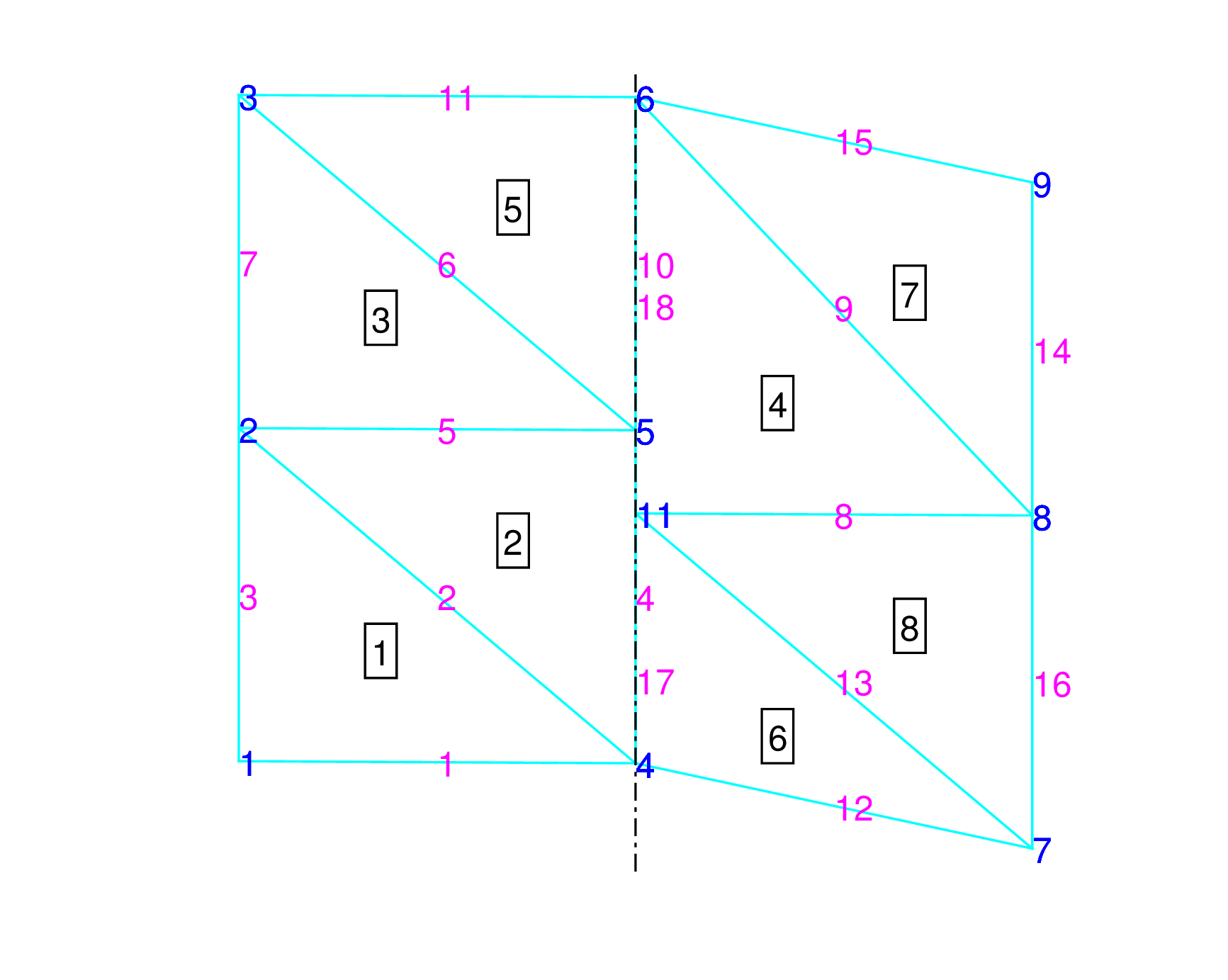
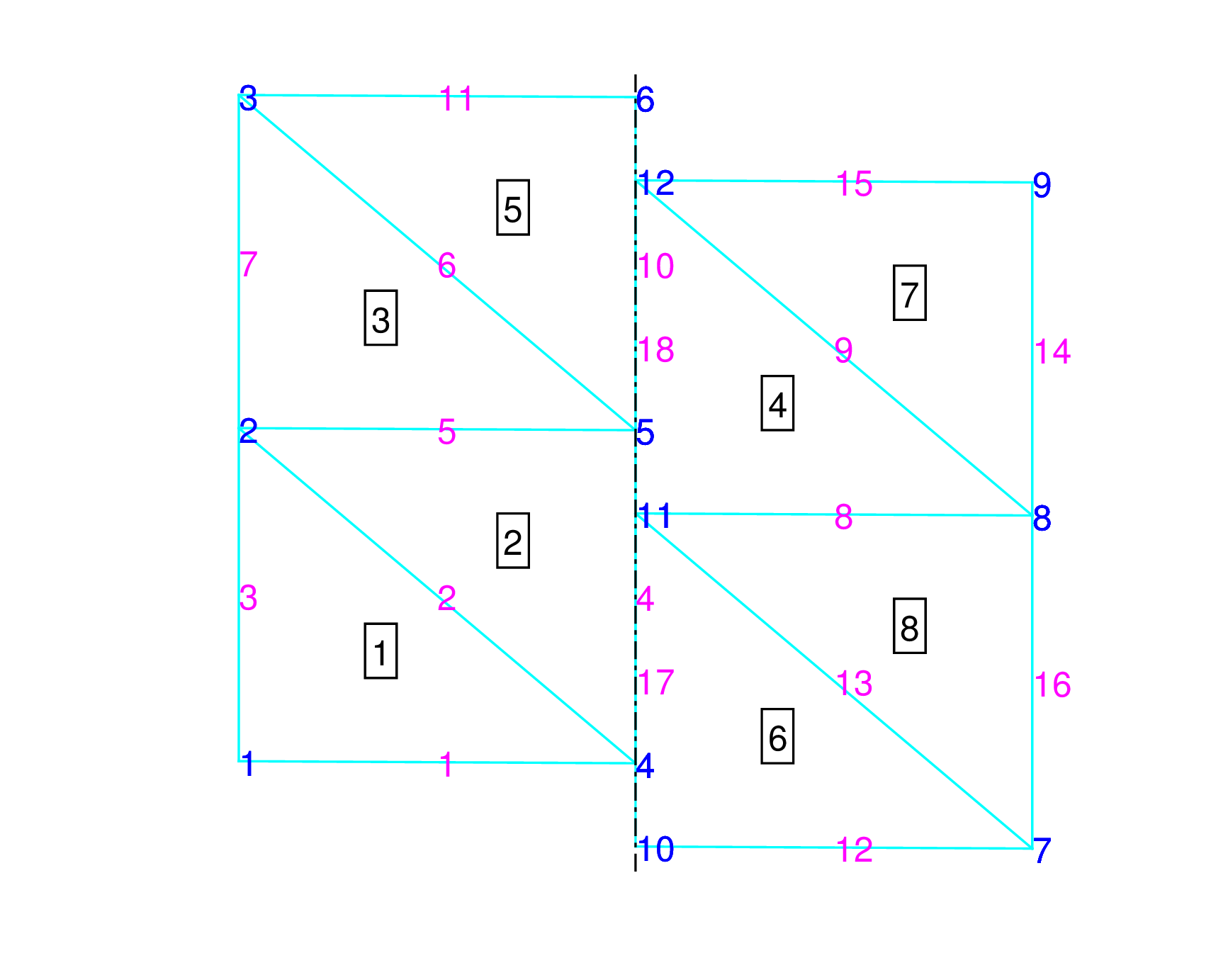
First, in matrix tri we substitute with in all the right elements; moreover, we consider matrix Vertex2Elem and in row we leave only the left elements and we put the others in row (because now is no more a vertex for the right neighbors).
Then we have to deal with the edges: if we need to substitute with a new edge . In matrix Elem2Edge all the right neighbors change with , and in matrix Edge2Elem we insert a new row equal to row (the new edge inherits all the characteristics from the old one). The same has to be done if . The endpoints of these new edges are the endpoints of the substituted edges seen from the right (so basically there is instead of ). The endpoints of the left edges do not change. Besides we add as intermediate point in and as intermediate point of , (note that an edge is allowed to have more than one intermediate point). In this way also matrix Edge2Vertex has been updated. Matrix Vertex2Edge is easily modified at the same time.
Finally, we have to revise the list of neighbors: in particular the edges that gained an intermediate point ( and ) gain also neighbors. In particular the new neighbors of are the left neighbors of and the new neighbors of are the right neighbors of . This allow us to update Edge2Elem and Elem2Edge.
At the end we mark with a label the nodes which are intermediate for an edge: we call them hanging nodes and they are constrained to move along that edge. Note that in the case of straight slip-lines no distinction between master and slave nodes is required, since both will move along the same straight interface. To extend the algorithm to the case of piece-wise linear interfaces, this distinction is introduced in such a way that only slave nodes will be constrained to slide along edges, while the master nodes can move freely. For some first preliminary results concerning the extension to completely general slide lines, see Section 4 of this paper.
2.5.2 Hanging nodes
Consider a hanging node which lies on the edge : it is at the interface and it is a vertex only of elements lying on one side of the interface, so its Voronoi neighbors are in the same smooth region. However it is not free to move everywhere but it must slide along that edge, to avoid creation of holes or superposition of elements in the mesh.
We apply the averaged node solver of Cheng and Shu among its Voronoi neighbors, we find its new coordinates and we project them over edge , obtaining . Now, we compute also the new coordinates of the other points over edge . If two of them are sufficiently close, we decide to merge them (see section 2.5.3), otherwise the computed coordinates are the new coordinates of such a node and no update of the connectivity matrices is required.
2.5.3 Fusion of two existing nodes


Suppose we computed the new coordinates at time of all the nodes over the same edge denoted by , which are assumed to be already projected onto the straight line spanned by edge . If the new coordinates of two of them, say and , are too close, we decide to merge them. Moreover, if one intermediate node of edge falls outside the edge, we decide to merge it with the closest endpoint of the edge.
Since the loop over the nodes is carried out according to the increasing global numbering of the nodes, we decide to remove the node with the largest global number (we call it dead node, ) because we have not worked with it yet, and to maintain the one with the smallest global numbering (call it fusion node, ) assigning to it as new coordinates the average between and
| (34) |
We assign the same coordinates also to the dead node
| (35) |
Now, we need to update the connectivity tables. See also Figure 4 to follow our construction.
This process is somehow more complicated than the nodes splitting. Indeed when we insert a new node at time we only add information without losing anything about the previous time step, and even if it is true that the right neighbors of a doubled node change their node with a new one , we can dispose of all its reference simply by giving to at time the same coordinates of , see also (31). On the contrary, when we remove a node we lose all the reference to it, reference that, only for time , we still need during the computation of the interface fluxes in the finite volume scheme (it is for this reason that in (35) we have assigned the coordinates even to the dead node). So we decide to duplicate some of the connectivity tables, creating triNew, Elem2EdgeNew, Edge2ElemNew, Edge2VertexNew, and Vertex2ElemNew. During the insertion procedure we modify in the same way both the old and the new matrices, while during the fusion we modify only the new matrices. Hence we can use the old ones in the finite volume scheme, because they store all the needed information (for example they refer both to the dead and the fusion node which have the same coordinates at the new time ), while when we advance in time, to , we maintain updated only the new ones because the information about two previous time steps are no longer necessary and so we can overwrite the old connectivity matrices with the new ones.
First, in matrix triNew we substitute with in all the neighbors of the dead node; moreover, we consider matrix Vertex2ElemNew, in row we put both the neighbors of the dead and the fusion node and we nullify row . We do the same with matrix Vertex2EdgeNew: we nullify row and we put in row all the edges that contain or .
Then all the edges that contain substitute it with (in matrix Edge2VertexNew), whereas the edges with both and (that we memorize in a list Edge[dn-fn]) remove . We note that merging and we are removing the segment in between, so we look for the edges that contain it (listed in Edge[dn-fn]) and its neighbor elements that we list in Elem[dn-fn]. We update now matrix Edge2ElemNew because the edges in Edge[dn-fn] have no more one of the neighbors in Elem[dn-fn] .
Afterward we check if the absence of this segment makes some edges in Edge[dn-fn] equal: in this case we remove one of them (the one with the largest global number) and we update correspondingly the new connectivity matrices.
Besides we modify the labels telling us if a node is hung to some edges and which nodes and edges are currently existing. This last passage prevents us to work again with disappeared nodes and allows us to reuse their global numbering when we want to insert a new node or a new edge.
3 Numerical results
In this section, we solve a large set of numerical tests in order to validate the presented nonconforming direct ALE scheme. The robustness of the method is checked both on smooth and discontinuous problems related to the shallow water equations written in Cartesian and in polar coordinates. The test cases are carried out using either the Rusanov or the Osher type flux, the value of in (26) is always taken equal to unless otherwise specified, and the CFL number is chosen as CFL. Furthermore, the order of convergence is verified first fixing for the mesh motion an arbitrary velocity, then in the case of a steady vortex in equilibrium using the local fluid velocity.
3.1 Sanity checks: pure sliding
The numerical examples reported in this section are sanity checks testing the ability of the method to detect and maintain straight slip-line interfaces. We consider the shallow water equations, which can be cast into form (1) with
| (36) |
The initial computational domain is given by . First, we take the initial condition
| (37) |
which also coincides with the exact solution at any time. We impose wall boundary conditions on the left and on the right side of the domain, respectively, whereas at the top and at the bottom of the domain we impose transmissive boundary conditions. In Figure 5 we show the numerical results over a triangular mesh and then over a mixed mesh composed of both, triangular and quadrilateral elements. The chosen mesh velocity coincides exactly with the fluid velocity, as in a pure Lagrangian context. At each time step we have verified that the total water volume is conserved up to machine precision both locally and globally and that relation (25), the GCL, is verified also up to machine precision.


Next, we consider as initial condition
| (38) |
with denoting the lower Gauss bracket, and we run our algorithm until a final time with different threshold values, see (26), in such a way that there will be a different number of interfaces along which nodes have to be doubled and merged in time. The discretization of the computational domain is reported in Figure 6. Also in this case we reach the exact solution (that is the initial condition translated in the motion direction), the total volume of water is conserved and relation (25) is verified up to machine precision at each time step and on each element.
Finally, we want to show that the interface can be along any straight line (provided that edges lie over this line): we take as initial condition
| (39) |
and in Figure 7 we report the computational domain at different times. Again, the numerical solution matches the exact one and as expected, the total volume is conserved and equation (25) is satisfied up to machine precision.
3.2 Periodic boundary conditions


The tests reported in the previous section can be run also by imposing periodic boundary conditions on the top and at the bottom of the computational domain. In Figure 8 we show the discretization of the computational domain at time for the initial conditions in (37) and in (38). We would like to underline that no distortion of the mesh elements appears even after a very long computational time, and as a direct consequence the time steps remain almost constant during the computation. As always in this type of test cases the volume conservation holds and the numerical solution is equal to the exact one up to machine precision.
3.3 Riemann problem
Let us now consider as initial condition a Riemann problem with a discontinuity in the water level
| (40) |
that originates a left-traveling rarefaction fan and a right-moving shock wave. We decided to move the mesh with an arbitrary mesh velocity function
in order to check the robustness of the algorithm also in the presence of discontinuities. We imposed periodic boundary conditions on the top and on the bottom of the square, and wall boundary conditions on the left and on the right. The final discretization of the computational domain together with the comparison between the numerical and the exact solution are depicted in Figure 9 both for the first order accurate scheme (i.e. without the MUSCL-Hancock strategy for the reconstruction) and the second order accurate scheme.
 |
 |
 |
3.4 Convergence test
 |
 |
 |
| mesh points | mesh points | ||||||
|---|---|---|---|---|---|---|---|
| 12 12 | 1.95E-01 | 1.44E-01 | - | 12 12 | 1.95E-01 | 4.96E-02 | - |
| 24 24 | 9.78E-02 | 7.58E-02 | 0.93 | 24 24 | 9.78E-02 | 1.23E-02 | 2.02 |
| 40 40 | 5.88E-02 | 4.69E-02 | 0.94 | 40 40 | 5.88E-02 | 4.24E-03 | 2.10 |
| 80 80 | 2.95E-02 | 2.41E-02 | 0.97 | 80 80 | 2.95E-02 | 1.01E-03 | 2.09 |
| 120 120 | 1.98E-02 | 1.62E-02 | 0.99 | 120 120 | 1.98E-02 | 4.51E-04 | 2.01 |
To verify the order of convergence of the proposed method we study the passive transport of a quantity , that at time is taken equal to a Gaussian profile and then will be passively transported in the direction of the fluid flow without changing its shape. The PDE system describing this situation is obtained from the standard shallow water equations (36) with the addition of the concentration of a passive tracer,
| (41) |
We fix the following initial condition
| (42) |
where we use a fluid velocity of and where we have taken the period . The mesh is moved with the velocity
| (43) |
according to the ALE framework, where the mesh velocity can be chosen arbitrarily. We prescribed periodic boundary conditions on the upper and lower side of the rectangular domain, and wall boundary conditions on the left and right sides.
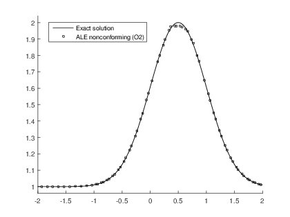
Since the exact solution is known () and it is smooth, we can verify the order of convergence of our method. In Table 1 we report the order of convergence of the basic first order finite volume method, and of its second order extension that uses the MUSCL-Hancock strategy for the reconstruction procedure in space and time. Moreover, in Figure 10 we compare the numerical solution for the variable with the profile of the exact solution and we show the mesh at the final time.
3.5 Steady vortex in equilibrium
To show that our method is also robust enough for vortex flows, we simulate the case of a steady vortex in equilibrium and we will compare the results obtained with our nonconforming method with a standard conforming algorithm (without any rezoning technique) looking at the differences after long simulation times. First, we rewrite the shallow water equations (36) in polar coordinates. Consider the usual relation between polar and Cartesian coordinates
| (44) |
and the corresponding relations for the derivatives
| (45) |
and let and be respectively the radial and the tangential component of the velocity, linked to and by
| (46) |
Now by substituting into (36) the expressions given in (46) and (45), after some calculations, we derive a new set of hyperbolic equations which, however, does not yet fit into the general form (1), since the fluxes in the above system depend explicitly on the spatial coordinate (i.e. the system is not autonomous). Thus, we add the trivial equation to the system, obtaining finally
| (47) | |||
| (48) | |||
| (49) | |||
| (50) |
The vector of the conserved variables, the non linear flux, and the source can now be written as
| (51) |
and the Jacobian matrices, necessary for the computation of the ALE Jacobian matrix in (19), are
| (52) |
We choose the following initial condition
| (53) |
which is a stationary solution of (50), and so coincides with the exact solution at any time. We performed our test both with the Osher and the Rusanov fluxes and with a mesh made of triangles, quadrilaterals or both.
The considered computational domain is which is easily mapped to the annulus with radius . Indeed the choice of considering the shallow water equations in polar coordinates allows us to study the vortex over a rectangular domain with periodic boundary conditions (at and ) instead of dealing with circles. At and we have imposed reflective boundary conditions. In particular using the polar coordinates the detected shear interfaces lie over straight lines and so they are perfectly handled by our algorithm. The images presented in this section are then obtained by mapping back our results to Cartesian coordinates, as shown in Figure 11.
First, Table 2 confirms the designed order of convergence of our algorithm in multiple situations: so primarily we can say that the mesh motion does not affect the standard order of convergence of the MUSCL-Hancock strategy and moreover this shows once again that the numerical flux computation, even at the nonconforming interfaces, is carried out correctly. The numerical solution at is compared with the analytical one in Figure 12.
Then we compare the results with a standard conforming method. First, let us underline that when the velocity changes even within the same element the only way to overcome the mesh distortion would be to split the element itself. For this reason, where the velocity field changes smoothly and as a consequence the shear flow affects all the vertices of the same element, at a certain time the mesh will become invalid even in the nonconforming case. This would not happen if the velocity field were uniform within each element, i.e. if each element moved all its vertices with the same velocity, e.g. the velocity of the barycenter.
The main difference between the new nonconforming algorithm and a conventional conforming method is the final time at which the computation stops due to an invalid mesh, and the time step restriction that depends on the smallest encircle diameter of the elements.
In Table 3 we report the employed number of time steps and their dimension for different kinds of meshes and at different times. We remark that a larger value of decreases the required number of time steps and in this way also the total amount of computational time. The last results of each group refer to the moment at which the algorithm breaks due to an invalid mesh: one can easily see that the nonconforming method is able to run almost eight times longer than a conventional ALE method on conforming grids.
Finally, looking at Figure 13 one can appreciate that the conforming method destroys the mesh immediately and then breaks, whereas the new nonconforming algorithm maintains a high quality mesh for a very long time, even with a very coarse mesh.


 |
 |
 |
 |
 |
 |
| , Osher flux, quadrilateral elements | , Rusanov flux, triangular elements | ||||||
|---|---|---|---|---|---|---|---|
| mesh points | mesh points | ||||||
| 12 12 | 2.33E-01 | 1.36E-03 | - | 20 20 | 7.18E-02 | 5.97E-04 | - |
| 24 24 | 1.17E-01 | 3.42E-04 | 1.99 | 30 30 | 5.21E-02 | 2.54E-04 | 2.11 |
| 32 32 | 8.74E-02 | 1.94E-04 | 1.97 | 40 40 | 3.91E-02 | 1.43E-04 | 2.01 |
| 44 44 | 6.36E-02 | 1.03E-04 | 1.98 | 55 55 | 2.84E-02 | 7.76E-05 | 1.91 |
| 60 60 | 4.66E-02 | 5.57E-05 | 1.99 | 60 60 | 2.60E-02 | 6.58E-05 | 1.91 |
| 216 | 264 | 300 | |||||||
| conforming algorithm | |||||||||
| 1 | 110 | 9.58E-03 | 1 | 180 | 5.40E-03 | 1 | 180 | 5.71E-03 | |
| 8 | 1163 | 4.13E-03 | 8 | 2180 | 2.52E-03 | 10 | 2071 | 3.11E-03 | |
| 12 | 2370 | 2.70E-03 | 12 | 4035 | 1.89E-03 | 15 | 4098 | 2.04E-03 | |
| stop at | 15.3 | 3773 | 2.06E-03 | 15.5 | 6072 | 1.54E-03 | 17 | 5190 | 1.78E-03 |
| nonconforming algorithm | |||||||||
| 1 | 110 | 9.58E-03 | 1 | 180 | 5.82E-03 | 1 | 175 | 5.68E-03 | |
| 8 | 851 | 9.50E-03 | 8 | 1410 | 5.52E-03 | 10 | 1720 | 5.92E-03 | |
| 30 | 3175 | 9.30E-03 | 30 | 6033 | 4.06E-03 | 15 | 2565 | 5.94E-03 | |
| 60 | 7757 | 4.90E-03 | 60 | 15010 | 2.84E-03 | 80 | 15979 | 3.34E-03 | |
| stop at | 119 | 26430 | 2.24E-03 | 129 | 35791 | 1.94E-03 | 132 | 36275 | 2.13E-03 |
4 Extension to general slide lines
All test problems shown before were limited to logically straight slide lines. However, there is no intrinsic limitation to logically straight slide lines in our algorithm, since the integral space-time conservation form (17) of the conservation law is valid for arbitrary closed space-time control volumes. This simple, elegant but at the same time very powerful formulation allows also to dynamically add and remove elements or to change their type during the simulation in a consistent manner that respects the GCL as well as local and global conservation. All these features are trivially built in by construction, due to the integral formulation on closed space-time control volumes. In Figure 14 we show examples of space-time control volumes that result when elements change type or when elements are dynamically added and removed during a simulation. For logically non-straight slide lines, it is necessary to divide elements and nodes into masters and slaves, where the master elements maintain their number of nodes, while the slave elements must in general change their element type during the sliding process. Also note that master nodes are free to move anywhere, while slave nodes must slide along the master edges. Furthermore, small elements need to be removed if they lead to excessively small time steps due to the CFL condition. We now repeat the same shallow water vortex test problem as described in the previous section, but using the PDE in Cartesian coordinates. This leads to logically non-straight slide lines. The comparison between the classical conforming moving mesh algorithm and the new nonconforming approach presented in this paper is shown in Fig. 15 and Table 4. We observe the improved mesh quality and time step size compared to the classical conforming approach, in particular when the moving nonconforming mesh is combined with the removal of small elements. The obtained results look promising and justify further research in this direction in the future.

 |
 |
 |
 |
 |
 |
 |
 |
 |
 |
 |
 |
| Time step size | |||
| time | conforming | nonconforming | nonconforming + |
| element removal | |||
| 0.3 | 3.8E-3 | 3.2E-3 | 3.2E-2 |
| 0.6 | 3.6E-3 | 2.1E-3 | 2.1E-3 |
| 1.0 | 1.9E-3 | 9.0E-4 | 1.2E-3 |
| 1.3 | 5.8E-4 | 1.2E-4 | 1.4E-3 |
| 1.7 | - | - | 1.4E-3 |
5 Well balancing for the shallow water equations in polar coordinates
At this point we are able to maintain a high quality mesh even in the case of strong shear flows, and to preserve the physical properties of the system (mass, momentum, energy) for very long computational times. Moreover, thanks to the use of a Lagrangian framework, our novel method is little dissipative for contact discontinuities.
The aim of this last section is to extend the algorithm in such a way that in addition it can preserve also exactly (i.e. up to machine precision) certain relevant and non-trivial equilibrium solutions. In particular, our interest is focused on the shallow water equations in cylindrical coordinates given by (51), where the presence of a source term makes this task quite challenging.
The procedures that allow to preserve some equilibrium of interest are called well balanced methods. We refer to [62, 25] and the references therein for a theoretical framework. For well-balanced schemes in the presence of gravity, see e.g. [18, 27, 1].
The importance of these techniques is related to the fact that conventional numerical schemes in which the source term may be discretized in a consistent manner are not able to preserve certain stationary solutions of the PDE, especially on coarse meshes. This leads to erroneous numerical solutions when trying to compute small perturbations around the stationary solution necessitating the need for very fine meshes.
For example, the initial data considered in the previous test case (53) represents a stationary solution for the system, characterized by the equilibrium between the centrifugal and the gravitational forces. But this precise balancing has to be achieved also at the numerical level in order to preserve the stationary solutions. And this is not trivial, especially because the two forces appear one in the flux and the other one in the source term, and consequently in classical finite volume schemes, they are discretized in a different way, making it almost impossible to maintain a precise balancing between them.
Following the ideas presented in [62] and [45], we decide to rewrite the source terms in (51) by means of nonconservative products in order to take them into account directly in the flux computation. The general form of the obtained system is
| (54) |
where, with respect to (1), we have the additional matrix which collects the nonconservative terms written using the standard conserved variables and some other trivially conserved variables added to the system. To clarify our notation, we want to remark that with we mean the vector of conserved variables defined in the space of the admissible states , and with we mean the value of the conserved variables obtained through a reconstruction procedure inside each element. (For a first order method in the control volume simply coincides with the cell average of element ).
System (51) can be cast in form (54) by adding as auxiliary variables the radius and the bottom topography such that the free surface is . The involved terms are the following
| (55) |
The main difficulty of systems written in this form, both from the theoretical and the numerical point of view, comes from the presence of nonconservative products that do not make sense in the distributional framework when the solution develops discontinuities. From the theoretical point of view, in this paper we assume the definition of nonconservative products as Borel measures given in [32]. This definition, which depends on the choice of a family of paths in the phase space, allows one to give a rigorous definition of weak solutions of (54).
We consider here the discretization of system (54) by means of a numerical scheme which is path-conservative in the sense introduced in [62], and that can be cast in our space–time formulation as follows
| (56) |
where represents an extension of the nonconservative matrix in the time direction
and represents a well balanced space–time flux function augmented by the jump terms for the non-conservative product, which is explicitly designed to preserve certain equilibrium solutions of the PDE exactly at the discrete level. For all the other terms the same notation of Section 2.2 holds.
The rest of this section is organized as follows. We start giving the expression of the well balanced space–time flux function which is already enough to define a first order scheme. Then will give some hints about the extension of the well balanced techniques to second order and, we conclude presenting some numerical results.
5.1 Well balanced space–time flux function
The core of the well balanced method is the design of the well balanced space–time flux function. Its final expression will be
| (57) |
where the term represents a well balanced way to write the nonconservative products, and is the viscosity term that we will derive slightly modifying the Osher flux.
and are defined in terms of a family of paths , . In this paper, we want to choose a family of paths in such a way that stationary solutions of the shallow water equations (51) given by
| (58) |
are preserved.
In general, according to the theory of [32], the family of paths should be a Lipschitz continuous family of functions , satisfying some regularity and compatibility conditions, in particular
| (59) |
Moreover, according to [62], the numerical flux should satisfy the following properties:
| (60) |
and also for all , ,
| (61) |
where
| (62) |
with the same notations of (19). In particular should satisfy
| (63) |
Note that if the standard segment path, that is
is prescribed for all the variables, then the resulting scheme is not well balanced. Here we propose a family of paths that is connected to the known equilibrium profiles for the free surface and the angular velocity , whereas for the other variables the segment path is sufficient. Let be a reparametrization of a stationary solution given by (58) that connects the two equilibrium states with , then we define as follows
| (64) |
where and and
That is is a segment path on the fluctuations with respect to a stationary solution. With this choice, it is clear that if and lie on the same stationary solution satisfying (58), then and , reduces to . In such situation we have that and
Therefore
For the sake of simplicity, in the following we will use the notation instead of when there is no confusion.
Let us now define in the general case, where and do not lie on a stationary solution. In such case we have that
| (65) |
It is clear from the definition of that . What is interesting is the discretization of the second term that can be rewritten as
| (66) |
where is any known profile for the angular velocity at the equilibrium; moreover call a primitive of , i.e. In this way we obtain that
where for variables and we can employ a standard segment path to connect the left and the right states
Instead, following the idea in (64) and considering the terms in (66) we define
| (67) |
which exploits the reparametrization of at the equilibrium and approximates with a segment path the fluctuations of the angular velocity
A similar approach is used for defined as
Taking into account that
could be rewritten as follows
| (68) |
Note that
therefore reduces to
where we have employed the mid point rule to approximate the integrals and the following notation holds . Finally, term could be approximated in the same way. Nevertheless, as this terms explicitly depends on and we are interested to preserve equilibria with , a more simple approach could be used. Thus, could be defined as
| (69) |
which vanishes when . As pointed out in [62], a sufficient condition for a first order path-conservative scheme to be well balanced is that
| (70) |
if and lie on the same stationary solution. Therefore, with the previous choice of paths, this quantity is zero if . In the next paragraph we propose a slightly modified version of the Osher flux which results to be well balanced.
5.2 Osher Romberg viscosity matrix
The numerical viscosity term associated to the standard path-conservative Osher scheme [40] reads
| (71) |
with . For the numerical approximation of the viscosity matrix, first we notice that it can be written as
| (72) |
and then, we approximate the previous expression by a quadrature formula as follows:
Now, we propose to approximate by the following expression:
where is a Roe-matrix associated to the system (see [62] for details), that is a matrix satisfying
| (73) |
where is defined as in the previous section using the states and . Therefore, the viscosity term reads as follows:
| (74) |
where
| (75) |
Note that if and lie on the same stationary solution and , , so vanishes. Therefore, the proposed numerical scheme is exactly well balacend for stationary solutions given by (58).
Here, as quadrature rule, we propose the Romberg method with and
With this choice, the viscosity term of the Osher-Romberg method results as follows:
| (76) | ||||
Note that the mayor drawback in the previous expression is that the complete eigenstructure of the Jacobian matrix (62) should be computed as
| (77) |
where is the diagonal matrix of the sign of the eigenvalues of , is the matrix of the right-eigenvectors and its inverse. As counter part, the Osher-Romberg method is little dissipative and is stable under the standard CFL condition.
The extension to higher order of accuracy is also possible: for example, to obtain a second order method it suffices to slightly modify the MUSCL reconstruction procedure of Section 2.1. The basic idea is again to define the reconstruction operator as a combination of a smooth stationary solution together with a standard reconstruction operator to reconstruct the fluctuations with respect to the given stationary solution. The extension of the well balanced procedures to higher order of accuracy will be the object of another work. However for a complete presentation of the general framework one can refer to the work of Castro et al. in [24].
5.3 Numerical Results
In this section, first we want to show that the well balanced method really works in general situations and not only close to the equilibria of the system. In this way, it will be clear that it can be applied in any context without corrupting the standard characteristics of the scheme, and it will perform better than classical schemes when near to a prescribed equilibrium. Then, we will see that the coupling between our nonconforming techniques with the well balanced strategy allow us to study the vortex flow of Section 3.5 even for longer periods of time.
5.3.1 Riemann problem
To show the correctness of our method we solve a classical Riemann problem with our well balanced Osher-Romberg ALE scheme. We consider the system of equation in (51), and as computational domain . We impose the following initial conditions
| (78) |
with . The results at the final computational time are shown in Figure 16, where we report a cut along . The method, even if it is set up to preserve the smooth stationary profile described in Section 3.5, converges properly to the reference solution of this problem, despite the presence of discontinuities.

5.3.2 Steady vortex in equilibrium
Test A.
Let us consider again the test case of Section 3.5, with the initial condition of (53). The coupling between our novel nonconforming ALE scheme together with the well balanced techniques gives us, even after a very long computational time, a good mesh quality (see Figure 17) and a numerical solution equal to the exact one up to machine precision (refer to Table 5).
Note that we have employed a mesh of squares with the constraints that interfaces lie over straight lines with constant radius. This automatically implies that each square of the mesh has two edges parallel to the axis: over this kind of edges the component of the flux does not play any role, and so the method is well balanced simply because the component of the flux is zero for stationary vortex-type solutions and (65) has been proved to be discretized in the correct way. The other two edges are parallel between them, so at the equilibrium, fluxes through them cancel.
Test B.
Moreover, to show that the method is able to preserve any known stationary solution that satisfies the constraint in (58), we have performed a similar test but starting from a different stationary condition
| (79) |
over the same computational domain . Even in this case the numerical solution remains close to the exact one up to machine precision for very long times, as also shown in Table 5.


| Test A | Test B | ||||
|---|---|---|---|---|---|
| points | points | ||||
| points | error | time | error | time | error |
| 12 6 | 1.42E-14 | 10 | 1.28E-14 | 10 | 2.11E-13 |
| 16 8 | 1.28E-14 | 50 | 3.74E-14 | 100 | 4.84E-13 |
| 24 12 | 3.04E-14 | 150 | 4.02E-14 | 150 | 3.25E-13 |
| 36 18 | 6.68E-14 | 200 | 4.88E-14 | 200 | 2.62E-13 |
6 Conclusion
We have developed a robust second order direct ALE finite volume scheme on moving unstructured nonconforming meshes. The main focus was on straight slip-line interfaces, but the approach can also easily be extended to general slide lines. In this paper, only some preliminary results for general slide lines have been shown, in order to provide a proof of concept. Further research in this direction is necessary. The presented results show that the method reaches its designed order of convergence and its overall accuracy. In particular, a high quality mesh is maintained and as a direct consequence the time step remains almost constant during the computation and the total amount of required computational effort is reduced, despite the increased algorithmic complexity of the numerical scheme on nonconforming meshes. Furthermore, even with straight slip-lines, the proposed method is already able to deal with sufficiently complex situations. In particular, if coupled with the presented well-balanced techniques it can be also considered for practical applications, for example in the context of the compressible Euler equations of gasdynamics with gravity, which are highly relevant in computational astrophysics, e.g. for the simulation of accretion discs and rotating gas clouds around compact objects like stars, neutron stars or black holes.
In future research we plan to extend the presented method to better than second order of accuracy by extending the ADER-WENO and ADER-DG ALE schemes [16, 13, 14, 15] to moving nonconforming unstructured meshes. Further research may also concern the incorporation of time accurate local time-steping (LTS) [38, 17, 26] into our algorithm.
Dedication
The new numerical method introduced in this paper is dedicated to Prof. Eleuterio Francisco Toro at the occasion of his 70th birthday and in honor of his groundbreaking scientific contributions to the field of shock capturing methods for computational fluid dynamics.
Acknowledgments
The research presented in this paper has been partially financed by the European Research Council (ERC) under the European Union’s Seventh Framework Programme (FP7/2007-2013) with the research project STiMulUs, ERC Grant agreement no. 278267. This research has been also supported by the Spanish Government and FEDER through the research project MTM2015-70490-C2-1-R and the Andalusian Government research projects P11-FQM-8179 and P11-RNM-7069. Moreover this project has received funding from the European Union’s Horizon 2020 research and innovation Programme under the Marie Sklodowska-Curie grant agreement no. 642768.
References
- [1] Well-balanced schemes for the euler equations with gravitation.
- [2] D. Balsara. A two-dimensional HLLC Riemann solver for conservation laws: Application to Euler and magnetohydrodynamic flows. Journal of Computational Physics, 231:7476–7503, 2012.
- [3] D.S. Balsara. Multidimensional Riemann problem with self-similar internal structure – Part I – Application to hyperbolic conservation laws on structured meshes. Journal of Computational Physics, 277:163–200, 2014.
- [4] D.S. Balsara and M. Dumbser. Multidimensional Riemann problem with self-similar internal structure – Part II – Application to hyperbolic conservation laws on unstructured meshes. Journal of Computational Physics, 287:269–292, 2015.
- [5] D.S. Balsara, M. Dumbser, and R. Abgrall. Multidimensional HLLC Riemann Solver for Unstructured Meshes - With Application to Euler and MHD Flows. Journal of Computational Physics, 261:172–208, 2014.
- [6] A.J. Barlow and J. Whittle. Mesh adaptivity and material interface algorithms in a two dimensional Lagrangian hydrocode. Chemical Physics, 19:15–26, 2000.
- [7] T.J. Barth and D.C. Jespersen. The design and application of upwind schemes on unstructured meshes. AIAA Paper 89-0366, pages 1–12, 1989.
- [8] M. Berndt, J. Breil, S. Galera, M. Kucharik, P.H. Maire, and M. Shashkov. Two–step hybrid conservative remapping for multimaterial arbitrary Lagrangian�-Eulerian methods. Journal of Computational Physics, 230:6664–6687, 2011.
- [9] S. Bertoluzza, S. Del Pino, and E. Labourasse. A conservative slide line method for cell-centered semi-Lagrangian and ALE schemes in 2D. ESAIM: Mathematical Modelling and Numerical Analysis (M2AN), 50:187–214, 2016.
- [10] G. Blanchard and R. Loubère. High order accurate conservative remapping scheme on polygonal meshes using a posteriori MOOD limiting. Computers and Fluids, 136:83–103, 2016.
- [11] P. Bochev, D. Ridzal, and M.J. Shashkov. Fast optimization-based conservative remap of scalar fields through aggregate mass transfer. Journal of Computational Physics, 246:37–57, 2013.
- [12] W. Boscheri, D.S. Balsara, and M. Dumbser. Lagrangian ADER-WENO finite volume schemes on unstructured triangular meshes based on genuinely multidimensional HLL Riemann solvers. Journal of Computational Physics, 267:112–138, 2014.
- [13] W. Boscheri and M. Dumbser. Arbitrary–Lagrangian–Eulerian one–step WENO finite volume schemes on unstructured triangular meshes. Communications in Computational Physics, 14:1174–1206, 2013.
- [14] W. Boscheri and M. Dumbser. A direct Arbitrary-Lagrangian-Eulerian ADER-WENO finite volume scheme on unstructured tetrahedral meshes for conservative and non-conservative hyperbolic systems in 3d. Journal of Computational Physics, 275:484 – 523, 2014.
- [15] W. Boscheri and M. Dumbser. Arbitrary–Lagrangian–Eulerian discontinuous Galerkin schemes with a posteriori subcell finite volume limiting on moving unstructured meshes. Journal of Computational Physics, 346:449–479, 2017.
- [16] W. Boscheri, M. Dumbser, and D.S. Balsara. High order Lagrangian ADER-WENO schemes on unstructured meshes – application of several node solvers to hydrodynamics and magnetohydrodynamics. International Journal for Numerical Methods in Fluids, 76:737–778, 2014.
- [17] W. Boscheri, M. Dumbser, and O. Zanotti. High order cell-centered Lagrangian-type finite volume schemes with time-accurate local time stepping on unstructured triangular meshes. Journal of Computational Physics, 291:120–150, 2015.
- [18] N. Botta, R. Klein, S. Langenberg, and S. Lützenkirchen. Well balanced finite volume methods for nearly hydrostatic flows. Journal of Computational Physics, 196:539–565, 2004.
- [19] J. Breil, T. Harribey, P.H. Maire, and M. Shashkov. A multi-material ReALE method with MOF interface reconstruction. Computers and Fluids, 83:115–125, 2013.
- [20] E.J. Caramana. The implementation of slide lines as a combined force and velocity boundary condition. Journal of Computational Physics, 228:3911–3916, 2009.
- [21] E.J. Caramana, D.E. Burton, M.J. Shashkov, and P.P. Whalen. The construction of compatible hydrodynamics algorithms utilizing conservation of total energy. Journal of Computational Physics, 146:227–262, 1998.
- [22] E.J. Caramana and M.J. Shashkov. Elimination of artificial grid distorsion and hourglass–type motions by means of Lagrangian subzonal masses and pressures. Journal of Computational Physics, 142:521–561, 1998.
- [23] G. Carré, S. Del Pino, B. Després, and E. Labourasse. A cell-centered Lagrangian hydrodynamics scheme on general unstructured meshes in arbitrary dimension. Journal of Computational Physics, 228:5160–5183, 2009.
- [24] M. Castro, J.M. Gallardo, J.A. López-García, and C. Parés. Well–balanced high order extensions of Godunov’s method for semilinear balance laws. SIAM Journal on Numerical Analysis, 46(2):1012–1039, 2008.
- [25] M.J. Castro, J.M. Gallardo, and C. Parés. High-order finite volume schemes based on reconstruction of states for solving hyperbolic systems with nonconservative products. Applications to shallow-water systems. Mathematics of Computation, 75:1103–1134, 2006.
- [26] J.R. Cavalcanti, M. Dumbser, D. da Motta-Marques, and C.R. Fragoso Junior. A conservative finite volume scheme with time-accurate local time stepping for scalar transport on unstructured grids. Advances in Water Resources, 86:217–230, 2015.
- [27] P. Chandrashekar and C. Klingenberg. A second order well-balanced finite volume scheme for Euler equations with gravity. SIAM Journal on Scientific Computing , 37:B382–B402, 2015.
- [28] J. Cheng and C.W. Shu. A high order ENO conservative Lagrangian type scheme for the compressible Euler equations. Journal of Computational Physics, 227:1567–1596, 2007.
- [29] J. Cheng and E.F. Toro. A 1D conservative Lagrangian ADER scheme. Chinese Journal of Computational Physics, 30:501–508, 2013.
- [30] G. Clair, B. Despres, and E. Labourasse. A new method to introduce constraints in cell-centered Lagrangian schemes. Computer Methods in Applied Mechanics and Engineering, 261-262:56–65, 2013.
- [31] G. Clair, B. Despres, and E. Labourasse. A one-mesh method for the cell-centered discretization of sliding. Computer Methods in Applied Mechanics and Engineering, 269:315–333, 2014.
- [32] G. Dal Maso, P.G. LeFloch, and F. Murat. Definition and weak stability of nonconservative products. J. Math. Pures Appl. , 74:483–548, 1995.
- [33] B. Després and C. Mazeran. Symmetrization of Lagrangian gas dynamic in dimension two and multidimensional solvers. C.R. Mecanique, 331:475–480, 2003.
- [34] B. Després and C. Mazeran. Lagrangian gas dynamics in two-dimensions and Lagrangian systems. Archive for Rational Mechanics and Analysis, 178:327–372, 2005.
- [35] V.A. Dobrev, T.E. Ellis, T.V. Kolev, and R.N. Rieben. Curvilinear finite elements for Lagrangian hydrodynamics. International Journal for Numerical Methods in Fluids, 65:1295–1310, 2011.
- [36] V.A. Dobrev, T.E. Ellis, T.V. Kolev, and R.N. Rieben. High order curvilinear finite elements for Lagrangian hydrodynamics. SIAM Journal on Scientific Computing, 34:606–641, 2012.
- [37] V.A. Dobrev, T.E. Ellis, Tz.V. Kolev, and R.N. Rieben. High order curvilinear finite elements for axisymmetric Lagrangian hydrodynamics. Computers and Fluids, 83:58–69, 2013.
- [38] M. Dumbser. Arbitrary–Lagrangian–Eulerian ADER–WENO finite volume schemes with time–accurate local time stepping for hyperbolic conservation laws. Computer Methods in Applied Mechanics and Engineering, 280:57–83, 2014.
- [39] M. Dumbser and E. F. Toro. On universal Osher–type schemes for general nonlinear hyperbolic conservation laws. Communications in Computational Physics, 10:635–671, 2011.
- [40] M. Dumbser and E. F. Toro. A simple extension of the Osher Riemann solver to non-conservative hyperbolic systems. Journal of Scientific Computing, 48:70–88, 2011.
- [41] M. Dumbser, A. Uuriintsetseg, and O. Zanotti. On Arbitrary–Lagrangian–Eulerian one–step WENO schemes for stiff hyperbolic balance laws. Communications in Computational Physics, 14:301–327, 2013.
- [42] F.Vilar. Cell-centered discontinuous Galerkin discretization for two-dimensional Lagrangian hydrodynamics. Computers and Fluids, 64:64–73, 2012.
- [43] F.Vilar, P.H. Maire, and R. Abgrall. Cell-centered discontinuous Galerkin discretizations for two-dimensional scalar conservation laws on unstructured grids and for one-dimensional Lagrangian hydrodynamics. Computers and Fluids, 46(1):498–604, 2010.
- [44] F.Vilar, P.H. Maire, and R. Abgrall. A discontinuous Galerkin discretization for solving the two-dimensional gas dynamics equations written under total Lagrangian formulation on general unstructured grids. Journal of Computational Physics, 276:188–234, 2014.
- [45] J.M. Gallardo, C. Parés, and M.J. Castro. On a well-balanced high-order finite volume scheme for shallow water equations with topography and dry areas. Journal of Computational Physics, 227:574–601, 2007.
- [46] S.K. Godunov. Finite difference methods for the computation of discontinuous solutions of the equations of fluid dynamics. Mathematics of the USSR: Sbornik, 47:271–306, 1959.
- [47] M. Kucharik, R. Liska, J. Limpouch, and P. Váchal. ALE simulations of high-velocity impact problem. Journal of Computational Physics, 76:737–778, 2014.
- [48] M. Kucharik, R. Loubère, L. Bednàrik, and R. Liska. Enhancement of Lagrangian slide lines as a combined force and velocity boundary condition. Computers & Fluids, 83:3–14, 2013.
- [49] M. Kucharik and M.J. Shashkov. One-step hybrid remapping algorithm for multi-material arbitrary Lagrangian-Eulerian methods. Journal of Computational Physics, 231:2851–2864, 2012.
- [50] Z. Li, X. Yu, and Z. Jia. The cell–centered discontinuous Galerkin method for Lagrangian compressible Euler equations in two dimensions. Computers and Fluids, 96:152–164, 2014.
- [51] W. Liu, J. Cheng, and C.W. Shu. High order conservative Lagrangian schemes with Lax–Wendroff type time discretization for the compressible Euler equations. Journal of Computational Physics, 228:8872–8891, 2009.
- [52] R. Loubère, M. Dumbser, and S. Diot. A new family of high order unstructured MOOD and ADER finite volume schemes for multidimensional systems of hyperbolic conservation law. Communications in Computational Physics, 16:718–763, 2014.
- [53] R. Loubère, P.H. Maire, and P. Váchal. A second-order compatible staggered Lagrangian hydrodynamics scheme using a cell-centered multidimensional approximate Riemann solver. Procedia Computer Science, 1:1931–1939, 2010.
- [54] R. Loubère, P.H. Maire, and P. Váchal. 3D staggered Lagrangian hydrodynamics scheme with cell-centered Riemann solver-based artificial viscosity. International Journal for Numerical Methods in Fluids, 72:22–42, 2013.
- [55] R. Loubère and M.J. Shashkov. A subcell remapping method on staggered polygonal grids for arbitrary–lagrangian–eulerian methods. Journal of Computational Physics, 23:155–160, 2004.
- [56] P.H. Maire. A high-order cell-centered Lagrangian scheme for two-dimensional compressible fluid flows on unstructured meshes. Journal of Computational Physics, 228:2391–2425, 2009.
- [57] P.H. Maire. A high-order one-step sub-cell force-based discretization for cell-centered Lagrangian hydrodynamics on polygonal grids. Computers and Fluids, 46(1):341–347, 2011.
- [58] P.H. Maire. A unified sub-cell force-based discretization for cell-centered Lagrangian hydrodynamics on polygonal grids. International Journal for Numerical Methods in Fluids, 65:1281–1294, 2011.
- [59] P.H. Maire, R. Abgrall, J. Breil, and J. Ovadia. A cell-centered Lagrangian scheme for two-dimensional compressible flow problems. SIAM Journal on Scientific Computing, 29:1781–1824, 2007.
- [60] C.D. Munz. On Godunov–type schemes for Lagrangian gas dynamics. SIAM Journal on Numerical Analysis, 31:17–42, 1994.
- [61] A. López Ortega and G. Scovazzi. A geometrically–conservative, synchronized, flux–corrected remap for arbitrary Lagrangian–Eulerian computations with nodal finite elements. Journal of Computational Physics, 230:6709–6741, 2011.
- [62] C. Parés. Numerical methods for nonconservative hyperbolic systems: a theoretical framework. SIAM Journal on Numerical Analysis, 44:300–321, 2006.
- [63] S. Del Pino. A curvilinear finite-volume method to solve compressible gas dynamics in semi-Lagrangian coordinates. Comptes Rendus de l’Académie des Sciences - Series I - Mathematics, 348:1027–1032, 2010.
- [64] G. Scovazzi. Lagrangian shock hydrodynamics on tetrahedral meshes: A stable and accurate variational multiscale approach. Journal of Computational Physics, 231:8029–8069, 2012.
- [65] V. Springel. E pur si muove: Galilean-invariant cosmological hydrodynamical simulations on a moving mesh. Monthly Notices of the Royal Astronomical Society, 401(2):791–851, 2010.
- [66] E.F. Toro. Riemann Solvers and Numerical Methods for Fluid Dynamics. Springer, second edition, 1999.
- [67] B. van Leer. Towards the ultimate conservative difference scheme II: Monotonicity and conservation combined in a second order scheme. Journal of Computational Physics, 14:361–370, 1974.
- [68] J. von Neumann and R.D. Richtmyer. A method for the calculation of hydrodynamics shocks. Journal of Applied Physics, 21:232–237, 1950.
- [69] M. L. Wilkins. Calculation of elastic-plastic flow. Methods in Computational Physics, 3, 1964.
- [70] Y.V. Yanilkin, E.A. Goncharov, V.Y. Kolobyanin, V.V. Sadchikov, J.R. Kamm, M.J. Shashkov, and W.J. Rider. Multi-material pressure relaxation methods for Lagrangian hydrodynamics. Computers and Fluids, 83:137–143, 2013.