Bayesian Estimates of Astronomical Time Delays between Gravitationally Lensed Stochastic Light Curves

We plot a pair of simulated light curves from a doubly-lensed quasar in Figure 2; the light curves are labeled as $A$ and $B$. Each observation time is denoted by vertical dashed lines, at which the observer measures the brightness of each gravitationally lensed quasar image. In a real data analysis, these images would correspond to the two bright sources in the second panel of Figure 1. The brightness is reported on the magnitude scale, an astronomical logarithmic measure of brightness, in which smaller numbers correspond to brighter objects. The magnitudes in Figure 2 are presented up to an overall additive calibration constant as was the case in the TDC. Since the time delay is estimated via relative comparison between fluctuations in the two light curves, our analysis is insensitive to this overall additive constant.

For a doubly-lensed quasar, there are four variables recorded on an irregularly spaced sequence of observation times $\boldsymbol{t}=(t_{1},t_{2},\ldots,t_{n})^{\top}$; the observed magnitudes $\boldsymbol{x}=(x_{1},x_{2},\ldots,x_{n})^{\top}$ for light curve $A$ and $\boldsymbol{y}=(y_{1},y_{2},\ldots,y_{n})^{\top}$ for light curve $B$ as well as standard deviations, $\boldsymbol{\delta}=(\delta_{1},\delta_{2},\ldots,\delta_{n})^{\top}$ and $\boldsymbol{\eta}=(\eta_{1},\eta_{2},\ldots,\eta_{n})^{\top}$, representing their uncertainties due to heteroskedastic measurement error. In Figure 2, $\boldsymbol{x}$ and $\boldsymbol{y}$ are represented by red squares and blue circles, and their standard deviations by the half lengths of vertical lines around the symbols. Similarly, for a quadruply-lensed quasar, there are four light curves, each with their own measurement errors.

Since a quasar exhibits fluctuations in its brightness, it is possible to estimate time delays between different views of those fluctuations. In Figure 2, for example, the bottom of the V-shaped valley of light curve $A$ at around 900 days precedes that of light curve $B$ by around 50 days. Other features in the light curves exhibit a similar time shift of about 50 days.

However, a number of aspects of the light curves in Figure 2 make accurate time delay estimation statistically challenging. First, irregular observation times are inevitable because observations may be prevented in poor weather or during the day. Second, the motion of the Earth around the Sun causes seasonal gaps because the part of the sky containing the quasar is not visible at night from the location of a particular telescope during certain months. Third, since the light of each gravitationally lensed image traverses different paths through the gravitational potential, they are subject to differing degrees of lensing magnification. Thus, the light curves often exhibit different average magnitudes. Finally, observed magnitudes are measured with error, leading to relatively larger measurement errors for fainter images.

Moreover, some quasar images exhibit additional independent extrinsic variability, an effect called microlensing²² 2 Microlensing is conceptually similar to strong lensing except that the lens is a star moving within the intervening galaxy. However, the lensed images produced by microlensing cannot be separately seen because their angular separation is too small for us to resolve with a telescope. Instead, astronomers observe only the combined magnification of both images, which changes with time due to the relative motions of the source and lensing star.. Significant microlensing occurs when a path of light passes unusually close to a star that is moving within the lensing galaxy. Lensing by this star introduces independent brightness magnification variations into the corresponding image in addition to the overall magnifications caused by strong lensing of the galaxy (Chang and Refsdal, 1979; Tewes, Courbin and Meylan, 2013). The timescale of the microlensing variability is typically much larger than that of the intrinsic quasar variability if the lens is on a galaxy scale (Liao et al., 2015). Thus the individual light curves may exhibit different long-term trends that are not related to the intrinsic variability of the source³³ 3 MacLeod et al. (2010) who analyzed about 9,000 quasars obtained from the Sloan Digital Sky Survey (Berk et al., 2004) show that the timescale of quasar intrinsic variability varies from days to years, and Mosquera and Kochanek (2011) indicate that the five shortest timescales of microlensing among 87 lensed quasars are between 8 and 12 years with respect to Einstein crossing timescales and are between 1 and 8 weeks with respect to source crossing timescale. Since the microlensing timescale is not always longer than the quasar intrinsic variability timescale, it is not always the case that we see the extrinsic long-term trends in the presence of microlensing.. In Figure 3, as an illustration, we plot the same simulated light curves $A$ and $B$ plotted in Figure 2 but with different added linear trends to simulate the effect of microlensing.

Conventional methods for time delay estimation have involved grid-based searches. One-dimensional grid methods estimate the time delay, $\Delta_{\textrm{AB}}$,⁴⁴ 4 A positive value of $\Delta_{\textrm{AB}}$ indicates that features in light curve $A$ appear before they appear in light curve $B$. by minimizing the $\chi^{2}$ distance or by maximizing the cross-correlation between two light curves, $\boldsymbol{x}$ and $\boldsymbol{y}_{\Delta_{\textrm{AB}}}$, on a grid of values of $\Delta_{\textrm{AB}}$ (Fassnacht et al., 1999), where $\boldsymbol{y}_{\Delta_{\textrm{AB}}}$ denotes $\boldsymbol{y}$ shifted by $\Delta_{\textrm{AB}}$ days to the right. Both techniques require an interpolation scheme. The dispersion method (Pelt et al., 1994) combines two light curves by shifting one of them in time and magnitude by $\Delta_{\textrm{AB}}$ and $\beta_{0}$, respectively. This is called the curve-shifting assumption. The method estimates $\Delta_{\textrm{AB}}$ and $\beta_{0}$ on a two dimensional grid by minimizing the sum of squared differences between consecutive pairs of magnitudes on the combined curve. A bootstrapping method is used to produce standard errors of the time delay estimates. These methods account only for the intrinsic variability of a quasar. (When it is clear from the context, we suppress the subscript on $\Delta_{\textrm{AB}}$ and simply use $\Delta$.)

Model-based methods have also been proposed in past to avoid the computational burden of evaluating the fit on a fine grid. For example, Tewes, Courbin and Meylan (2013) model the intrinsic and extrinsic variabilities of light curves using high-order and low-order splines, respectively. They obtain the least square estimate of $\Delta$ by iterating a two-step fitting routine in which splines are first fit given $\Delta$ and then $\Delta$ is optimized given the model fit. They also use parametric bootstrapping for the standard error of the time delay estimate.

Harva and Raychaudhury (2006, hereafter H&R) introduced the first fully Bayesian approach, though they do not account for microlensing. They assume each observed light curve is generated by an unobserved underlying process. One of the latent processes is assumed to be a shifted and scaled version of the other, with the time and magnitude shifts and the magnitude scale treated as unknown parameters. They use a collapsed Gibbs-type sampler for model fitting, with the latent process integrated out of the target posterior distribution. Unlike other existing methods this approach unifies parameter estimation and uncertainty quantification into a single coherent analysis based on the posterior distribution of $\Delta$.

The TDC motivated us to improve on H&R’s fully Bayesian model by taking advantage of modeling and computational advances made since H&R’s 2006 proposal. Specifically, we adopt an Ornstein-Uhlenbeck (O-U) process (Uhlenbeck and Ornstein, 1930) to model the latent light curve. The O-U process has been empirically shown to describe the stochastic variability of quasar data well (Kelly, Bechtold and Siemiginowska, 2009; Kozłowski et al., 2010; MacLeod et al., 2010; Zu et al., 2013). We address the effect of microlensing by incorporating a polynomial regression on time into the model. We specify scientifically motivated prior distributions and conduct a set of systematic sensitivity analyses; see Appendix E for details of the sensitivity analyses. In contrast to H&R’s strategy of sampling from a marginal distribution with the latent process integrated out, we use a Metropolis-Hastings (M-H) within Gibbs sampler (Tierney, 1994) to sample the posterior in the full parameter space. We improve the convergence rate of our MCMC (Markov chain Monte Carlo) sampler by using an ancilarity-sufficiency interweaving strategy (Yu and Meng, 2011) and adaptive MCMC (Brooks et al., 2011).

To complement the Bayesian method, we introduce a simple profile likelihood approach that allows us to remove nuisance parameters and focus on $\Delta$ (Davison, 2003, e.g., ). We show that the profile likelihood function of $\Delta$ is approximately proportional to the marginal posterior distribution of $\Delta$ when a Jeffreys’ prior is used for the nuisance parameters (Berger, Liseo and Wolpert, 1999), see Appendix D. For the problems we investigate the profile likelihood is nearly identical to the marginal posterior distribution in most cases, validating the approximation.

Our time delay estimation strategy combines these two complementary approaches. We first obtain the profile likelihood of $\Delta$, which is simple to compute. A more principled fully Bayesian analysis focuses on the dominant mode identified by the profile likelihood and provides joint inference for the time delay and other model parameters via the joint posterior distribution.

The rest of this paper is organized as follows. We describe our Bayesian model in Section 2 and the MCMC sampler that we use to fit it in Section 3. In Section 4, we introduce the profile likelihood approach. We then specify our estimation strategy and illustrate it via a set of numerical examples in Section 5. An R package, timedelay, that implements the Bayesian and profile likelihood methods is publicly available at CRAN⁵⁵ 5 https://cran.r-project.org/package=timedelay.

We assume that each time-delayed light curve is generated from a latent curve representing the true source magnitude in continuous time. We denote these latent curves by $\boldsymbol{X}=\{X(t),~t\in\mathbf{R}\}$ and $\boldsymbol{Y}=\{Y(t),~t\in\mathbf{R}\}$, respectively, where $X(t)$ and $Y(t)$ are unobserved true magnitudes at time $t$. We use the vector notation $\boldsymbol{X}(\boldsymbol{t})=(X(t_{1}),X(t_{2}),\ldots,X(t_{n}))^{\top}$ and $\boldsymbol{Y}(\boldsymbol{t})=(Y(t_{1}),Y(t_{2}),\ldots,Y(t_{n}))^{\top}$ to denote the $n$ magnitudes of each latent light curve at the irregularly-spaced observation times $\boldsymbol{t}$.

A curve-shifted model (Pelt et al., 1994; Kochanek et al., 2006) assumes that one of the latent light curves is a shifted version of the other, that is

where $\Delta$ is a shift in time and $\beta_{0}$ is a magnitude offset. For example, in Figure 4, we displayed the solid red and dashed blue latent curves of images A and B, respectively, generated under the model in (2.1). Thus the two curves exactly overlap if the solid red curve is shifted by $\Delta$ days and by $\beta_{0}$ magnitude units. (For illustration purposes, $\boldsymbol{X}$ is depicted as a solid red smooth curve; a more realistic model is described in Section 2.3.) The key advantage of this model is that a single latent light curve, here $\boldsymbol{X}$, is sufficient to represent the true magnitude time series of the two (or more) lensed images. This model is a special case of H&R’s scaled curve-shifted model, $Y(t)=sX(t-\Delta)+\beta_{0}$, where $s$ is a magnitude scale change, mentioned at the end of Section 1.2. Setting $s=1$ is reasonable because gravitational lensing only deflects the source light and magnifies it, i.e., multiplies the source flux. Because magnitude is on the $\log_{10}$ scale of source flux, we expect an additive offset, i.e., $\beta_{0}$, rather than a scale change. The curve-shifted model captures the essential physical effects of strong gravitational lensing (at least in the absence of microlensing), and thus is an appropriate model for estimating the time delay.

Microlensing causes additional long-term extrinsic variability unrelated to the intrinsic quasar variability driving the dynamics of $\boldsymbol{X}$. Thus, the curve-shifted model is not appropriate in the presence of microlensing. To account for microlensing, we assume that one of the latent light curves is a time-shifted version of the other, but with an additional polynomial regression of order $m$ on $t-\Delta$, that is

where $\boldsymbol{w}_{m}(t-\Delta)\equiv(1,t-\Delta,(t-\Delta)^{2},\ldots,(t-\Delta)^{m})^{\top}$ is a covariate vector of length $m+1$, and $\boldsymbol{\beta}\equiv\left(\beta_{0},\beta_{1},\beta_{2},\ldots,\beta_{m}\right)^{\top}$ is a vector of regression coefficients⁶⁶ 6 An orthonormal basis is more compatible with an independent prior on the regression coefficients and thus may be preferred if a higher degree polynomial regression is used.. The polynomial regression term in (2.2) accounts for the difference in the microlensing trends of the two light curves, i.e., the difference between the long-term trends of $Y(t)$ and $X(t-\Delta)$. The microlensing model in (2.2) reduces to a curve-shifted model in (2.1) if $\beta_{1}=\beta_{2}=\cdots=\beta_{m}=0$.

The best choice for the order of the polynomial regression depends on the extent of microlensing, and this varies from quasar to quasar. We set $m=3$ as a default because the third order polynomial regression has been successfully applied to model lensed quasars (Kochanek et al., 2006; Courbin et al., 2013; Morgan et al., 2012). If we find evidence via the profile likelihood that a third order polynomial regression is not sufficient to reduce the effect of microlensing (see Section 5.1 for details), we can impose a reasonable upper bound of $m$ by running preliminary regression on the observed light curves, and comparing the fits.

Observing the gravitationally-lensed images with a telescope, an astronomer measures the magnitude in each image, $x_{j}$ and $y_{j}$, and reports standard deviations, $\delta_{j}$ and $\eta_{j}$, representing the uncertainties of the magnitudes due to measurement errors⁷⁷ 7 The magnitude estimate and standard deviation typically summarize a Gaussian approximation to the likelihood of the latent magnitude for the flux data of an image. The standard deviation does not necessarily represent a standard error of a repeated sampling measurement error distribution. at time $t_{j}$, $j=1,2,\ldots,n$. We assume that these measurements have independent Gaussian errors centered at the latent magnitudes $X(t_{j})$ and $Y(t_{j})$, i.e.,

where $\textrm{N}[M,V]$ is a Gaussian distribution with mean $M$ and variance $V$, and $\boldsymbol{x}$ and $\boldsymbol{y}$ are independent given their true magnitudes. Using the model in (2.2), we can express (2.4) as

Given $\Delta$, we define $\boldsymbol{t}^{\Delta}=(t^{\Delta}_{1},t^{\Delta}_{2},\ldots,t^{\Delta}_{2n})^{\top}$ as the sorted vector of $2n$ times among the $n$ observation times, $\boldsymbol{t}$, and the $n$ time-delay-shifted observation times, $\boldsymbol{t}-\Delta$. Also, $\boldsymbol{X}(\boldsymbol{t}^{\Delta})=(X(t^{\Delta}_{1}),X(t^{\Delta}_{2}),\ldots,X(t^{\Delta}_{2n}))^{\top}$ is the vector of $2n$ latent magnitudes at the times in $\boldsymbol{t}^{\Delta}$. The joint density function of the observed data given $\boldsymbol{X}(\boldsymbol{t}^{\Delta})$, $\Delta$, and $\boldsymbol{\beta}$ is

where the two distributions in the product are given in (2.3) and (2.5).

We assume the latent continuous-time light curve, $\boldsymbol{X}$, is a realization of an O-U process (Uhlenbeck and Ornstein, 1930) as proposed in Kelly, Bechtold and Siemiginowska (2009). The stochastic differential equation,

defines the O-U process, where $\mu$ and $\sigma$ are on the magnitude scale and govern the overall mean and short-term variability of the underlying process, $\tau$ is a timescale (in days) for the process to revert to the long-term mean $\mu$, $\{B(t),~t\geq 0\}$ is a standard Brownian motion, and $dB(t)$ is an interval of the Brownian motion, whose distribution is Gaussian with mean zero and variance $dt$. We denote the three O-U parameters by $\boldsymbol{\theta}=(\mu,\sigma^{2},\tau)^{\top}$.

Kelly, Bechtold and Siemiginowska (2009) empirically demonstrated that the power spectrum of the O-U process is consistent with the mean power spectrum of 55 well-sampled quasar light curves at a specific frequency range with timescales shorter than $\tau$. They also investigated the associations between model parameters and the physical properties of quasars. For example, $\tau$ has a positive correlation with black hole mass, which is consistent with previous astrophysical studies. Kozłowski et al. (2010) and MacLeod et al. (2010) were concerned about a possible selection bias in the sample of quasars used in Kelly, Bechtold and Siemiginowska (2009) and thus they analyzed thousands of light curves. Kozłowski et al. (2010) found further support for the O-U process in their analyses of about 2,700 quasars obtained from the Optical Gravitational Lensing Experiment (Kozłowski and Kochanek, 2009, OGLE,). They showed that the distribution of the goodness of fit statistic obtained by fitting the O-U process to their light curves was consistent with the expected distribution of the statistic under the assumption that the light curve variation was stochastic. MacLeod et al. (2010) further verified the argument about the correlations between model parameters and physical properties in Kelly, Bechtold and Siemiginowska (2009) by analyzing about 9,000 quasars obtained from the Sloan Digital Sky Survey (Berk et al., 2004). Zu et al. (2013) also supported the O-U process by comparing it to the Gaussian process with three different covariance functions in fitting about 200 OGLE light curves. Their numerical results based on the $F$-test and Bayesian information criterion supported the O-U process. These studies popularized the O-U process among astrophysicists to the extent that the TDC simulated its quasar light curves under an O-U process⁸⁸ 8 The TDC organizers generated 500 10-year-long light curves by using the O-U process ($\mu=0$, $\log(\tau)\in[1.5,3.0]$, and $\log(\sigma)\in[-1.1,-0.3]$), and re-used these to make about 5,000 doubly- or quadruply-lensed light curves with different starting points, different seasonal gaps, etc. Microlensing is simulated via a catalog convergence of Oguri and Marshall (2010), shear, and surface density. The measurement errors were heteroskedastic Gaussian. The organizers intentionally contaminated the data to make the time delay estimation difficult; the reported standard deviations may be under-estimated, measurement errors may be correlated due to time-dependent calibration error, and magnitudes may be temporarily offset due to time-dependent systematic effects in the telescope optics. (Dobler et al., 2015). The earlier approach of H&R (2006) preceded these more recent advances in astrophysical and statistical modeling of quasars.

The solution of the stochastic differential equation in (2.7) provides the prior distribution for the time-sorted latent magnitudes $\boldsymbol{X}(\boldsymbol{t}^{\Delta})$ via its Markovian property. Specifically,

where $a_{j}\equiv\exp(-(t_{j}^{\Delta}-t_{j-1}^{\Delta})/\tau)$ is a shrinkage factor that depends on the observational cadence and $\tau$. If two adjacent latent magnitudes are close in time, i.e., $t_{j}^{\Delta}-t_{j-1}^{\Delta}$ is small, $a_{j}$ is close to unity and under this prior $X(t_{j}^{\Delta})$ borrows more information or shrinks more towards the previous latent magnitude, $X(t_{j-1}^{\Delta})$, and exhibits less uncertainty. On the other hand, if neighboring latent magnitudes are distant in time, e.g., due to a seasonal gap, $a_{j}$ is close to zero, and under this prior $X(t_{j}^{\Delta})$ borrows little information from the distant value $X(t_{j-1}^{\Delta})$ and instead approaches the overall mean $\mu$ with more uncertainty. This is known as the mean reversion property of the O-U process.

The joint prior density function of the $2n$ latent magnitudes is

where the distributions on the right-hand side are given in (2.8).

We adopt independent proper prior distributions for $\Delta$ and $\boldsymbol{\beta}$,

where $I_{\{D\}}$ is the indicator function of $D$, $\textrm{N}_{m+1}(\boldsymbol{\beta}\mid\boldsymbol{0},10^{5}\times I_{m+1})$ is an $m+1$ dimensional Gaussian density evaluated at $\boldsymbol{\beta}$ whose mean is $\boldsymbol{0}$, a vector of zeros with length $m+1$, and variance-covariance matrix is $10^{5}\times I_{m+1}$, with an $m+1$ dimensional identity matrix $I_{m+1}$. We put a diffuse Gaussian prior on $\boldsymbol{\beta}$ to minimize impact on the posterior inference and to ensure posterior propriety.

The range of the uniform prior distribution on $\Delta$, $[u_{1},u_{2}]$, reflects the range of interest. One choice is the entire feasible range (or feasible range) of $\Delta$, $[t_{1}-t_{n},t_{n}-t_{1}]$; only values of $\Delta$ in this range can correspond to adjusted light curves that overlap by at least one data point. (H&R uses a diffuse Gaussian prior distribution on $\Delta$ that is defined even outside this range.)

In some cases, information about the likely range of $\Delta$ is available from previous analyses or possibly from astrophysical probes. For example, we can find the likely range of $\Delta$ using a physical model for the mass and gravitational potential of the lens, as well as the redshifts (an astronomical measure of distance) and relative spatial locations of a quasar and lens.

In reality, the time delay and lensing magnification may be correlated a priori. We assume a priori independence, however, because it is difficult to construct an informative joint prior distribution without more information about the lens system, i.e., image positions, distances, and a lens model.

Considering both scientific knowledge and the dynamics of the O-U process, we put a uniform distribution on the O-U mean $\mu$, an independent inverse-Gamma (IG) distribution, IG(1, $b_{\sigma}$), on its short-term variance $\sigma^{2}$, and an independent IG(1, $b_{\tau}$) distribution on its timescale $\tau$, i.e.,

The units of $b_{\sigma}$ are magnitude squared per day, hereafter mag${}^{2}/$day, and the scale parameter of the IG distribution on $\tau$ is fixed at one day, i.e., $b_{\tau}=1$ day.

Here the uniform distribution on $\mu$ encompasses a magnitude range from that of the Sun (magnitude $=-26.74$) to that of the faintest object visible with the Hubble Space Telescope (magnitude $=30$). The IG distributions on $\tau$ and $\sigma^{2}$ set soft lower bounds⁹⁹ 9 Because the density function of IG($a,b$) decreases exponentially from its mode, $b/(a+1)$, toward zero and geometrically decreases with a power of $a+1$ towards infinity, it is relatively unlikely for the random variable to take on values much smaller than its mode. to focus on practical solutions in which $\Delta$ can be constrained. For example, in the limits when $\tau$ is much less than the observation cadence or when $\sigma^{2}$ is much smaller than the measurement variance divided by the cadence, the discrete observations of the continuous latent light curve appear as serially uncorrelated white noise sequence. In these limiting cases it is impossible to estimate $\Delta$ by matching serially correlated fluctuation patterns. The soft lower bounds for $\tau$ and $\sigma^{2}$ discount these limiting cases, and allow us to focus on the relevant parameter space in which we expect time delay estimation to be feasible.

We set the shape parameter of the IG prior distribution on $\tau$ to unity and the scale parameter $b_{\tau}$ to one day to obtain a weakly informative prior. The resulting soft lower bound on $\tau$ is 0.5 day and is smaller than all of the estimates of $\tau$ in MacLeod et al. (2010), who analyzed 9,275 quasars.

For the IG prior distribution of $\sigma^{2}$, we set the shape parameter to unity and the scale parameter to (Mean measurement standard deviation)² / (Median cadence), i.e.,

This scale parameter enables us to search for solutions for which we can constrain $\Delta$ by avoiding the above limiting case. Another viable choice for the scale parameter is $b_{\sigma}=2\times 10^{-7}$ because all estimates of $\sigma^{2}$ in MacLeod et al. (2010) are larger than this value. Sensitivity analyses for the choice of prior distributions of $\tau$ and $\sigma^{2}$ appear in Appendix E.

To improve the convergence rate of $\boldsymbol{\beta}$, we adopt the ancillarity-sufficiency interweaving strategy (Yu and Meng, 2011, ASIS,). In a general hierarchical modeling setting, ASIS interweaves trajectories of the Markov chains obtained by two discordant parameterizations of the unknown quantities, which reduces dependence between the adjoining iterates. A different parameterization for the location parameters, e.g., $\boldsymbol{\beta}$ in our case, can be derived by shifting, and that for scale parameters by rescaling. The two parameterizations are designed so that the original and transformed parameters can be viewed as ancillary and sufficient statistics for $\boldsymbol{\beta}$, respectively. ASIS is always faster to converge than the slower of the data augmentation samplers based on either of the two parameterizations and is geometrically convergent even when neither of the two data augmentation samplers is.

In the parameterization used up until now, $\boldsymbol{X}(\boldsymbol{t}^{\Delta})$ is an ancillary augmentation (AA) for $\boldsymbol{\beta}$ in that it is an ancillary statistic for $\boldsymbol{\beta}$. That is, the distribution of $\boldsymbol{X}(\boldsymbol{t}^{\Delta})$ in (2.8) does not depend on $\boldsymbol{\beta}$. On the other hand, a sufficiency augmentation (SA) for $\boldsymbol{\beta}$ is based on a transformation of $\boldsymbol{X}(\boldsymbol{t}^{\Delta})$ that have sufficient information to estimate $\boldsymbol{\beta}$, that is, a sufficient statistic for $\boldsymbol{\beta}$. To derive an SA for $\boldsymbol{\beta}$, we introduce the parameterization,

where

This indicator is one if $t^{\Delta}_{j}$ is an element of $\boldsymbol{t}-\Delta=\{t_{1}-\Delta,t_{2}-\Delta,\ldots,t_{n}-\Delta\}$ and zero otherwise. Thus, $\boldsymbol{K}(\boldsymbol{t}^{\Delta})$ represents the time-sorted latent magnitudes of $\boldsymbol{X}(\boldsymbol{t})$ and of microlensing-adjusted $\boldsymbol{Y}(\boldsymbol{t})$, i.e., $\boldsymbol{X}(\boldsymbol{t}-\Delta)+\boldsymbol{w}_{m}^{\top}(\boldsymbol{t}-\Delta)\boldsymbol{\beta}$. Using (3.7), we express the observation model in (2.3) and (2.5) as

The distributions for the latent light curve in (2.8) are replaced by

Under this reparameterization of the model in terms of $\boldsymbol{K}(\boldsymbol{t}^{\Delta})$, $\boldsymbol{\beta}$ appears only in (3.11), which means that $\boldsymbol{K}(\boldsymbol{t}^{\Delta})$ contains sufficient information to estimate $\boldsymbol{\beta}$ and thus $\boldsymbol{K}(\boldsymbol{t}^{\Delta})$ is an SA for $\boldsymbol{\beta}$. In contrast, $\boldsymbol{\beta}$ appears only in the distribution of observed magnitudes in (2.6), not in that of latent magnitudes in (2.8), and thus $\boldsymbol{X(t^{\Delta})}$ is an AA for $\boldsymbol{\beta}$. Because the parameterization does not affect the prior distributions of the model parameters in (2.10) and (2.11), the full joint posterior density in terms of $\boldsymbol{K}(\boldsymbol{t}^{\Delta})$, i.e., $p(\boldsymbol{K}(\boldsymbol{t}^{\Delta}),\Delta,\boldsymbol{\beta},\boldsymbol{\theta}\mid\boldsymbol{x},\boldsymbol{y})$, is proportional to the product of densities of observed data given in (3.9) and (3.10) and prior densities in (3.11), (2.10) and (2.11). Consequently, the marginal posterior distribution of the model parameters, $\{\Delta,\boldsymbol{\beta},\boldsymbol{\theta}\}$, is unchanged.

ASIS interweaves the trajectory of $\boldsymbol{\beta}$ from a sample constructed under AA and that constructed under SA. This can be accomplished by replacing Step 2 in (3.2) with the following four steps:

Again, we suppress the conditioning on $\boldsymbol{x}$ and $\boldsymbol{y}$. In Step 2_c, we set $\boldsymbol{\beta}^{(l)}$ to $\boldsymbol{\beta}^{(l)}_{\textrm{SA}}$ sampled from its conditional posterior distribution specified in (C.2). In Step 2_d, ASIS updates $\boldsymbol{X}^{(l)}(\boldsymbol{t}^{\Delta^{(l)}})$ to adjust for the inconsistency between the updates sampled in (3.3)–(3.5) that are based on $\boldsymbol{X}^{(l)}(\boldsymbol{t}^{\Delta^{(l)}})$ and the update $\boldsymbol{\beta}^{(l)}$ that is based on $\boldsymbol{K}^{(l)}(\boldsymbol{t}^{\Delta^{(l)}})$. Updating $\boldsymbol{X}^{(l)}(\boldsymbol{t}^{\Delta^{(l)}})$ in (3.15) synchronizes this inconsistency and preserves the stationary distribution (Yu and Meng, 2011). The additional computational cost of ASIS is negligible because the conditional updates in (3.12) and (3.14) include quick multivariate Gaussian sampling; see (C.1) and (C.2) for details.

ACFs of the model parameters obtained by MHwG equipped with ASIS, denoted by MHwG$+$ASIS, appear on the third row of Figure 5; the ACF of $\beta_{0}$ in the second column shows a noticeable improvement compared to that obtained by MHwG sampler. The ESS/sec for $\beta_{0}$ is 20.95 with MHwG$+$ASIS and 1.74 with MHwG. In general, ASIS improves the mixing of all the regression coefficients in our microlensing model. Although it improves the ACF for the components of $\boldsymbol{\beta}$, ASIS has little effect on the ACF of $\Delta$. The ESS/sec for $\Delta$ is 21.35 with MHwG$+$ASIS and 21.09 with MHwG. This small improvement implies that the dependence between $\Delta$ and $\boldsymbol{\beta}$ may be weak a posteriori; this is confirmed by our data analyses in Section 5.1. Nevertheless, ASIS improves overall convergence of the chain which we expect to improve the reliability of all inferences based on the chain.

Our MHwG sampler (either with or without ASIS) requires a proposal distribution in each of its two Metropolis steps, that is, N$\left[\Delta^{(l-1)},\psi^{2}\right]$ used to update $\Delta^{(l)}$ in (3.1) and N$\left[\log(\tau^{(l-1)}),\phi^{2}\right]$ used to update $\log(\tau^{(l)})$ in (3.5), where $\psi$ and $\phi$ are the proposal scales. To avoid burdensome off-line tuning of the proposal scales, we implement an adaptive MCMC sampler (Brooks et al., 2011) that allows automatic adjustment during the run. The steps of the adaptive MHwG+ASIS sampler are specified in Algorithm 1. Specifically, we implement an algorithm that updates the two proposal scales every 100 iterations, based on the most recent 100 proposals as outlined in Step 6 of Algorithm 1. The Markov chains equipped with the adaptive MCMC converge to the stationary distribution because the adjustment factors, $\exp(\pm\min(0.01,~1/\sqrt{i}))$, in Step 6 of of Algorithm 1 approach unity as $i$ goes to infinity. This condition is called diminishing adaptation condition (Roberts and Rosenthal, 2007). We set the lower and upper bounds of the acceptance rate to 0.23 and 0.44, respectively (Gelman et al., 2013).

All of the numerical results presented in Figure 5 were obtained using algorithms that similarly adapted their M-H updates, i.e., the M-H updates of all the parameters in CMHwG and of $\Delta$ and $\tau$ in both MHwG and MHwG+ASIS.

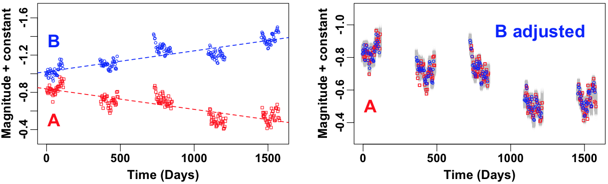
The simulated data for a doubly-lensed quasar are plotted in the first panel of Figure 6; the median cadence is 3 days, the cadence standard deviation is 1 day, observations are made for 4 months in each of 5 years for 200 observations in total, and measurement errors are heteroskedastic Gaussian. The light curves suffer from microlensing which can be identified from their different long-term linear trends and similar short-term (intrinsic) variability.

To show the effect of microlensing on the time delay estimation, we fit both the curve-shifted model ($m=0$) in (2.1) and the microlensing model with $m=3$ in (2.2). We plot $\log(L_{\textrm{prof}}(\Delta))$ and $L_{\textrm{prof}}(\Delta)$ based on the curve-shifted model over the feasible range, $[t_{1}-t_{n},~t_{n}-t_{1}]=[-1575.85,~1575.85]$, in the two panels of Figure 7. The profile likelihood exhibits large modes near the margins that overwhelm the profile likelihood near the true time delay (5.86 days denoted by the vertical dashed line).

In the presence of microlensing, the curve-shifted model cannot identify the time delay because the latent curves are not shifted versions of each other. The modes of $L_{\textrm{prof}}(\Delta)$ near the margins of the range of $\Delta$ occur because, in the small overlap between the tips of two light curves, spurious matches may be made by chance between similar fluctuation patterns. In Figure 8, for instance, we shift light curve $B$ in the $x$-axis by the three values of $\Delta$ indicated by three arrows in the second panel of Figure 7. In the first panel of Figure 8, the two light curves shifted by the true time delay do not match for any shift in magnitude. However, given the time delays at around $-1$,200 or 1,360 days, the two light curves look well-connected as shown in the second and third panels. Thus, the profile likelihood near the true time delay is overwhelmed by the values of the profile likelihood near $-1$,200 and 1,360 days.

To correct this effect, we fit the microlensing model with a third-order polynomial regression ($m=3$). Both $\log(L_{\textrm{prof}}(\Delta))$ and $L_{\textrm{prof}}(\Delta)$ are plotted in Figure 9. One mode clearly dominates $L_{\textrm{prof}}(\Delta)$. Using a uniform prior for $\Delta$ over its feasible range and setting $\sigma^{2}\sim\textrm{IG}(1,2/10^{7})$, we initialize three MCMC chains near $\hat{\Delta}_{\textrm{mean}}=6.36$ days. It took 14,457 seconds to map $L_{\textrm{prof}}(\Delta)$ and 5,115 seconds on average for each MCMC chain. The profile likelihood and marginal posterior near the dominant mode are almost identical and are consistent with the true value of $\Delta$ as shown in the third panel of Figure 9.

In the second panel of Figure 6, we combine two light curves by shifting light curve $B$ by the posterior mean of $\Delta$ in the horizontal axis and by subtracting the estimated polynomial regression based on the posterior means of $\boldsymbol{\beta}$ from light curve $B$. The microlensing model finds matches between the intrinsic fluctuations of the light curves after removing the relative microlensing trend from light curve $B$. We also plot the posterior sample of $\boldsymbol{X}(\boldsymbol{t}^{\Delta})$ in gray in the right panel of Figure 6. The gray regions represent the point-wise prediction intervals for the combined latent light curve. The gray areas encompass most of the combined observed light curve, indicating that the fitted model predicts the observed data well.

We summarize the Bayesian and profile likelihood estimates for $\Delta$ in Table 1. The true delay is within two posterior standard deviation of the posterior mean; similar accuracy is obtained with the profile likelihood approximation. This is anecdotal evidence that our model works well when microlensing is properly accounted for; there is no severe multi-modality near edges of the range of $\Delta$ in the second panel of Figure 9.

We also conduct a simulation study, generating 1,000 datasets from our final model with an adjustment for microlensing ($m=3$), and report the frequency coverage of the 95% posterior intervals (Tak, Kelly and Morris, 2017+). The result is over-coverage for $\Delta$, conservatively meeting the spirit of the frequentist confidence level, reasonable coverage for $\boldsymbol{\beta}$, and under-coverage for both $\sigma^{2}$ and $\tau$; see Table 2. The severe under-coverage for $\sigma^{2}$ does not seem to affect the coverage rate of $\Delta$; the scatter plot of $\Delta$ and $\log(\sigma)$ in Figure 10 indicates that the two parameters are almost independent a posteriori. In a numerical sensitivity analysis in Appendix E, we show that the posterior mode of $\Delta$ is close to the true time delay even when the posterior mode of $\log(\sigma)$ is substantially different from its true value. (See Figure 17 in Appendix E.)

Figure 10 displays scatterplots of the posterior sample of $\Delta$ against each of the other model parameters. The time delay $\Delta$ exhibits weak correlations with the regression coefficients and non-linear relationships with $\mu$ and $\log(\tau)$, though $\beta_{0}$ and $\log(\sigma)$ appear nearly independent of $\Delta$.

The simulated data for a quadruply-lensed quasar are plotted in Figure 11 and are composed of four light curves, $A,B,C$, and $D$; the median cadence is 6 days, the cadence standard deviation is 1 day, observations are made for 4 months in each of 10 years with 200 observations in total, and measurement errors are heteroskedastic Gaussian. The feasible range for each $\Delta$ is $[-3391.62,~3391.62]$.

With quadruply lensed data there are three time delay parameters because the four light curves are generated by one underlying process. Our model, however, is designed to analyze pairs of light curves independently, and thus we focus on $\Delta_{\textrm{AB}}$, $\Delta_{\textrm{AC}}$, and $\Delta_{\textrm{AD}}$, where the subscripts index the two light curves being compared, among the six possible pairs. This pair-wise approach proceeds by applying the method developed for doubly-lensed data in Section 5.1 to the pair of light curves corresponding to each of $\Delta_{\textrm{AB}}$, $\Delta_{\textrm{AC}}$, and $\Delta_{\textrm{AD}}$ in turn (Fassnacht et al., 1999).

By focusing on pairwise comparisons of the four time series, we do not account for the correlations between the time delays. A coherent model would consider all four light curves in a single model simultaneously (Hojjati, Kim and Linder, 2013; Tewes, Courbin and Meylan, 2013); the four light curves are generated from one latent process and the three distinct time delays may have a posteriori correlations. It is conceptually straightforward, but properly modeling quadruply lensed data would involve three time delays, 12 regression coefficients ($m=3$), and three O-U parameters. Extending our model to simultaneously consider all of the data is a topic for future research.

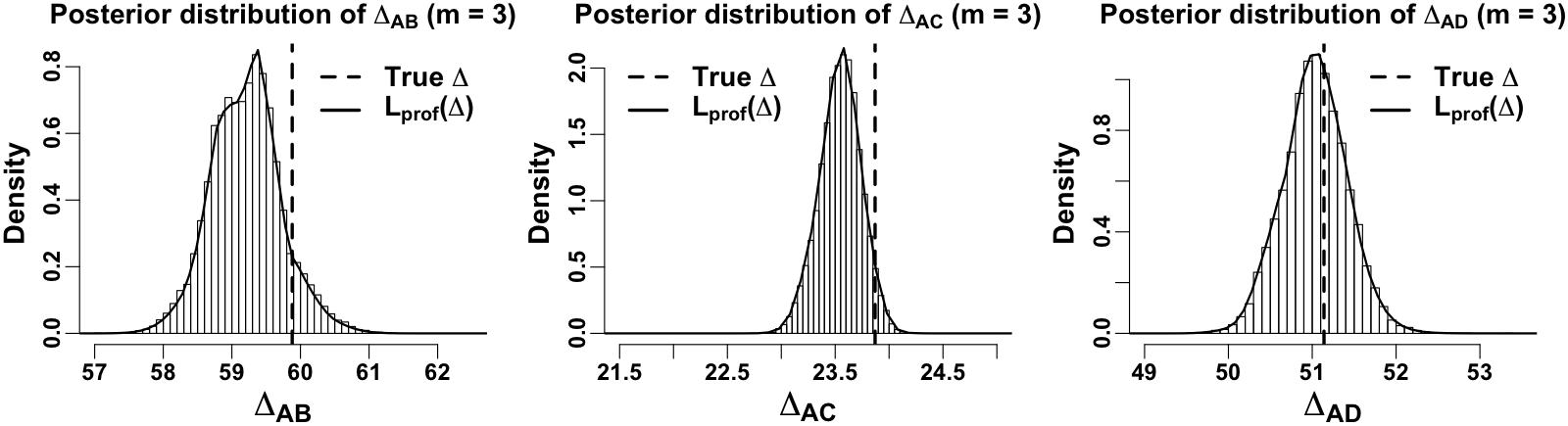
We analyze the quadruply lensed simulated light curves, using the microlensing model ($m=3$). After confirming a single dominating mode in the profile likelihood for each time delay parameter, we initiate three MCMC chains near this mode. The posterior distributions of $\Delta_{\textrm{AB}}$, $\Delta_{\textrm{AC}}$, and $\Delta_{\textrm{AD}}$ appear in Figure 12 with $L_{\textrm{prof}}(\Delta)$ superimposed. The profile likelihood is almost identical to the posterior distribution of each parameter and both estimate the true time delays well. The average CPU time taken to map $L_{\textrm{prof}}(\Delta)$ is about 73,000 seconds (averaging over the three time delays). The average CPU time taken for each MCMC chain is about 5,500 seconds (averaging over nine chains; three chains for each time delay). Our estimation results are summarized in Table 3. The Bayesian estimates and profile likelihood approximations are quite similar and both produce estimates within two standard deviations of the truth.

References

- Berger, Bernardo and Sun (2015) [author] Berger, J. O.J. O., Bernardo, J. M.J. M. and Sun, D.D. (2015). Overall Objective Priors. Bayesian Analysis 10 189–221.
- Berger, Liseo and Wolpert (1999) [author] Berger, J. O.J. O., Liseo, B.B. and Wolpert, R. L.R. L. (1999). Integrated Likelihood Methods for Eliminating Nuisance Parameters. Statistical Science 14 1–28.
- Berk et al. (2004) [author] Berk, D. E. V.D. E. V., Wilhite, Brian CB. C., Kron, Richard GR. G., Anderson, Scott FS. F., Brunner, Robert JR. J., Hall, Patrick BP. B., Ivezić, ŽeljkoŽ., Richards, Gordon TG. T., Schneider, Donald PD. P., York, Donald GD. G., Brinkmann, J. V.J. V., Lamb, D. Q.D. Q., Nichol, R. C.R. C. and Schlegel, D. J.D. J. (2004). The Ensemble Photometric Variability of 25,000 Quasars in the Sloan Digital Sky Survey. The Astrophysical Journal 601 692.
- Blandford and Narayan (1992) [author] Blandford, RDR. and Narayan, RR. (1992). Cosmological Applications of Gravitational Lensing. Annual Review of Astronomy & Astrophysics 30 311–358.
- Brooks et al. (1997) [author] Brooks, Stephen PS. P., Morgan, Byron JTB. J., Ridout, Martin SM. S. and Pack, SES. (1997). Finite Mixture Models for Proportions. Biometrics 53 1097–1115.
- Brooks et al. (2011) [author] Brooks, SteveS., Gelman, AndrewA., Jones, GalinG. and Meng, Xiao-LiX.-L. (2011). Handbook of Markov Chain Monte Carlo. CRC press.
- Chang and Refsdal (1979) [author] Chang, KK. and Refsdal, SS. (1979). Flux Variations of QSO 0957+561 A, B and Image Splitting by Stars Near the Light Path. Nature 282 561–564.
- LSST Science Collaboration (2009) [author] LSST Science Collaboration (2009). LSST Science Book, Version 2.0. arXiv:0912.0201.
- Courbin et al. (2013) [author] Courbin, FF., Chantry, VirginieV., Revaz, YY., Sluse, DD., Faure, CC., Tewes, MM., Eulaers, EvaE., Koleva, MM., Asfandiyarov, II., Dye, SS., Magain, P.P., van Winckel, H.H., Coles, J.J., Saha, P.P., Ibrahimov, M.M. and Meylan, G.G. (2013). COSMOGRAIL: the COSmological MOnitoring of GRAvItational Lenses IX. Time Delays, Lens Dynamics and Baryonic Fraction in HE 0435-1223. Astronomy & Astrophysics 536 A53.
- Davison (2003) [author] Davison, Anthony ChristopherA. C. (2003). Statistical Models. Cambridge University Press.
- Dobler et al. (2015) [author] Dobler, GregoryG., Fassnacht, ChristopherC., Treu, TommasoT., Marshall, Phillip JP. J., Liao, KaiK., Hojjati, AlirezaA., Linder, EricE. and Rumbaugh, NicholasN. (2015). Strong Lens Time Delay Challenge. I. Experimental Design. The Astrophysical Journal 799 168.
- Fassnacht et al. (1999) [author] Fassnacht, CDC., Pearson, TJT., Readhead, ACSA., Browne, IWAI., Koopmans, LVEL., Myers, STS. and Wilkinson, PNP. (1999). A Determination of Ho with the CLASS Gravitational Lens B1608+ 656. I. Time Delay Measurements with the VLA. The Astrophysical Journal 527 498.
- Fischer et al. (1997) [author] Fischer, P.P., Bernstein, G.G., Rhee, G.G. and Tyson, J. A.J. A. (1997). The Mass Distribution of the Cluster Q0957+561 from Gravitational Lensing. The Astronomical Journal 113 521.
- Fohlmeister et al. (2013) [author] Fohlmeister, JanineJ., Kochanek, Christopher SC. S., Falco, Emilio EE. E., Wambsganss, JoachimJ., Oguri, MasamuneM. and Dai, XinyuX. (2013). A Two-year Time Delay for the Lensed Quasar SDSS J1029+ 2623. The Astrophysical Journal 764 186.
- Gelman and Rubin (1992) [author] Gelman, AndrewA. and Rubin, Donald BD. B. (1992). Inference from Iterative Simulation Using Multiple Sequences. Statistical Science 7 457–472.
- Gelman et al. (2013) [author] Gelman, AndrewA., Carlin, John BJ. B., Stern, Hal SH. S., Dunson, David BD. B., Vehtari, AkiA. and Rubin, Donald BD. B. (2013). Bayesian Data Analysis. CRC press.
- Hainline et al. (2012) [author] Hainline, Laura JL. J., Morgan, Christopher WC. W., Beach, Joseph NJ. N., Kochanek, CSC., Harris, Hugh CH. C., Tilleman, TrudyT., Fadely, RossR., Falco, Emilio EE. E. and Le, Truong XT. X. (2012). A New Microlensing Event in the Doubly Imaged Quasar Q 0957+ 561. The Astrophysical Journal 744 104.
- Harva and Raychaudhury (2006) [author] Harva, MarkusM. and Raychaudhury, SomakS. (2006). Bayesian Estimation of Time Delays Between Unevenly Sampled Signals. IEEE.
- Hojjati, Kim and Linder (2013) [author] Hojjati, AlirezaA., Kim, Alex GA. G. and Linder, Eric VE. V. (2013). Robust Strong Lensing Time Delay Estimation. Physical Review D 87 123512.
- Inada et al. (2006) [author] Inada, NaohisaN., Oguri, MasamuneM., Morokuma, TomokiT., Doi, MamoruM., Yasuda, NaokiN., Becker, Robert HR. H., Richards, Gordon TG. T., Kochanek, Christopher SC. S., Kayo, IsshaI., Konishi, KohkiK. et al. (2006). SDSS J1029+ 2623: A Gravitationally Lensed Quasar with an Image Separation of 225. The Astrophysical Journal Letters 653 L97.
- Kelly, Bechtold and Siemiginowska (2009) [author] Kelly, Brandon CB. C., Bechtold, JillJ. and Siemiginowska, AnetaA. (2009). Are the Variations in Quasar Optical Flux Driven by Thermal Fluctuations? The Astrophysical Journal 698 895.
- Kochanek et al. (2006) [author] Kochanek, CSC., Morgan, NDN., Falco, EEE., McLeod, BAB., Winn, JNJ., Dembicky, JJ. and Ketzeback, BB. (2006). The Time Delays of Gravitational Lens HE 0435–1223: An Early-Type Galaxy with a Rising Rotation Curve. The Astrophysical Journal 640 47.
- Kozłowski and Kochanek (2009) [author] Kozłowski, SzymonS. and Kochanek, Christopher SC. S. (2009). Discovery of 5000 Active Galactic Nuclei Behind the Magellanic Clouds. The Astrophysical Journal 701 508.
- Kozłowski et al. (2010) [author] Kozłowski, SzymonS., Kochanek, Christopher SC. S., Udalski, AA., Soszyński, II., Szymański, MKM., Kubiak, MM., Pietrzyński, GG., Szewczyk, OO., Ulaczyk, KK. and Poleski, RR. (2010). Quantifying Quasar Variability as Part of a General Approach to Classifying Continuously Varying Sources. The Astrophysical Journal 708 927.
- Kumar, Stalin and Prabhu (2014) [author] Kumar, S RathnaS. R., Stalin, CSC. and Prabhu, TPT. (2014). H0 from 11 Well Measured Time-delay Lenses. Astronomy & Astrophysics 580 A38.
- Liao et al. (2015) [author] Liao, K.K., Treu, T.T., Marshall, P.P., Fassnacht, C. D.C. D., Rumbaugh, N.N., Dobler, G.G., Aghamousa, A.A., Bonvin, V.V., Courbin, F.F., Hojjati, A.A., Jackson, N.N., Kashyap, V.V., Rathna Kumar, S.S., Linder, E.E., Mandel, K.K., Meng, X. L.X. L., Meylan, G.G., Moustakas, L. A.L. A., Prabhu, T. P.T. P., Romero-Wolf, A.A., Shafieloo, A.A., Siemiginowska, A.A., Stalin, C. S.C. S., Tak, H.H., Tewes, M.M. and van Dyk, D.D. (2015). Strong Lens Time Delay Challenge: II. Results of TDC1. The Astrophysical Journal 800 11.
- Linder (2011) [author] Linder, Eric V.E. V. (2011). Lensing Time Delays and Cosmological Complementarity. Phys. Rev. D 84 123529. 10.1103/PhysRevD.84.123529
- Liu (2008) [author] Liu, Jun SJ. S. (2008). Monte Carlo Strategies in Scientific Computing. Springer Science & Business Media.
- MacLeod et al. (2010) [author] MacLeod, CLC., Ivezić, ŽŽ., Kochanek, CSC., Kozłowski, SS., Kelly, BB., Bullock, EE., Kimball, AA., Sesar, BB., Westman, DD., Brooks, KK., Gibson, R.R., Becker, A. C.A. C. and de Vries, W. H.W. H. (2010). Modeling the Time Variability of SDSS Stripe 82 Quasars as a Damped Random Walk. The Astrophysical Journal 721 1014.
- Morgan et al. (2012) [author] Morgan, Christopher WC. W., Hainline, Laura JL. J., Chen, BinB., Tewes, MalteM., Kochanek, Christopher SC. S., Dai, XinyuX., Kozlowski, SzymonS., Blackburne, Jeffrey AJ. A., Mosquera, Ana MA. M., Chartas, GeorgeG., Courbin, F.F. and Meylan, G.G. (2012). Further Evidence that Quasar X-ray Emitting Regions are Compact: X-ray and Optical Microlensing in the Lensed Quasar Q J0158-4325. The Astrophysical Journal 756 52.
- Mosquera and Kochanek (2011) [author] Mosquera, Ana MA. M. and Kochanek, Christopher SC. S. (2011). The Microlensing Properties of a Sample of 87 Lensed Quasars. The Astrophysical Journal 738 96.
- Munoz et al. (1998) [author] Munoz, JAJ., Falco, EEE., Kochanek, CSC., Lehár, JJ., McLeod, BAB., Impey, CDC., Rix, H-WH.-W. and Peng, CYC. (1998). The CASTLES project. Astrophysics and Space Science 263 51–54.
- Oguri and Marshall (2010) [author] Oguri, MasamuneM. and Marshall, Philip JP. J. (2010). Gravitationally Lensed Quasars and Supernovae in Future Wide-field Optical Imaging Surveys. Monthly Notices of the Royal Astronomical Society 405 2579–2593.
- Oscoz et al. (1997) [author] Oscoz, AlejandroA., Mediavilla, EvencioE., Goicoechea, Luis JulianL. J., Serra-Ricart, MiquelM. and Buitrago, JesusJ. (1997). Time Delay of QSO 0957+ 561 and Cosmological Implications. The Astrophysical Journal Letters 479 L89.
- Oscoz et al. (2001) [author] Oscoz, AA., Alcalde, DD., Serra-Ricart, MM., Mediavilla, EE., Abajas, CC., Barrena, RR., Licandro, JJ., Motta, VV. and Munoz, JAJ. (2001). Time Delay in QSO 0957+ 561 from 1984-1999 Optical Data. The Astrophysical Journal 552 81.
- Pelt et al. (1994) [author] Pelt, JJ., Hoff, WW., Kayser, RR., Refsdal, SS. and Schramm, TT. (1994). Time Delay Controversy on QSO 0957+ 561 not yet Decided. Astronomy & Astrophysics 286 775–785.
- Pelt et al. (1996) [author] Pelt, JaanJ., Kayser, RainerR., Refsdal, SjurS. and Schramm, ThomasT. (1996). The Light Curve and the Time Delay of QSO 0957+ 561. Astronomy & Astrophysics 305 97–106.
- Refsdal (1964) [author] Refsdal, SjurS. (1964). The Gravitational Lens Effect. Monthly Notices of the Royal Astronomical Society 128 295–306.
- Roberts and Rosenthal (2007) [author] Roberts, Gareth OG. O. and Rosenthal, Jeffrey SJ. S. (2007). Coupling and Ergodicity of Adaptive Markov Chain Monte Carlo Algorithms. Journal of Applied Probability 44 458–475.
- Schneider, Ehlers and Falco (1992) [author] Schneider, PP., Ehlers, JJ. and Falco, EEE. (1992). Gravitational Lenses. Springer.
- Schneider, Wambsganss and Kochanek (2006) [author] Schneider, PeterP., Wambsganss, JoachimJ. and Kochanek, Christopher SC. S. (2006). Gravitational Lensing: Strong, Weak and Micro. Springer.
- Serra-Ricart et al. (1999) [author] Serra-Ricart, MiquelM., Oscoz, AlejandroA., Sanchís, TeresaT., Mediavilla, EvencioE., Goicoechea, Luis JuliánL. J., Licandro, JavierJ., Alcalde, DavidD. and Gil-Merino, RodrigoR. (1999). BVRI Photometry of QSO 0957+ 561A, B: Observations, New Reduction Method, and Time Delay. The Astrophysical Journal 526 40.
- Shalyapin, Goicoechea and Gil-Merino (2014) [author] Shalyapin, VNV., Goicoechea, LJL. and Gil-Merino, RR. (2014). A 5.5-year Robotic Optical Monitoring of Q0957+ 561: Substructure in a Non-local cD Galaxy. Astronomy & Astrophysics 540 A132.
- Suyu et al. (2013) [author] Suyu, SHS., Auger, MWM., Hilbert, SS., Marshall, PJP., Tewes, MM., Treu, TT., Fassnacht, CDC., Koopmans, LVEL., Sluse, DD., Blandford, RDR., Courbin, F.F. and Meylan, G.G. (2013). Two Accurate Time-delay Distances from Strong Lensing: Implications for Cosmology. The Astrophysical Journal 766 70.
- Tak, Kelly and Morris (2017+) [author] Tak, H.H., Kelly, J.J. and Morris, C. N.C. N. (2017+). Rgbp: An R Package for Gaussian, Poisson, and Binomial Random Effects Models with Frequency Coverage Evaluations. Journal of Statistical Software arXiv:1612.01595.
- R Core Team (2016) R Core Team (2016). R: A Language and Environment for Statistical Computing R Foundation for Statistical Computing, Vienna, Austria.
- Tewes, Courbin and Meylan (2013) [author] Tewes, MM., Courbin, FF. and Meylan, GG. (2013). COSMOGRAIL: the COSmological MOnitoring of GRAvItational Lenses XI. Techniques for time delay measurement in presence of microlensing. The Astrophysical Journal 605 58.
- Tierney (1994) [author] Tierney, LukeL. (1994). Markov Chains for Exploring Posterior Distributions. The Annals of Statistics 22 1701–1728.
- Treu and Marshall (2016) [author] Treu, T.T. and Marshall, P. J.P. J. (2016). Time Delay Cosmography. The Astronomy and Astrophysics Review 24 11.
- Uhlenbeck and Ornstein (1930) [author] Uhlenbeck, George EG. E. and Ornstein, Leonard SalomonL. S. (1930). On the Theory of the Brownian Motion. Physical review 36 823.
- van Dyk and Meng (2001) [author] van Dyk, David AD. A. and Meng, Xiao-LiX.-L. (2001). The Art of Data Augmentation. Journal of Computational and Graphical Statistics 10 1–50.
- Walsh, Carswell and Weymann (1979) [author] Walsh, DD., Carswell, RFR. and Weymann, RJR. (1979). 0957+ 561 A, B- Twin Quasistellar Objects or Gravitational Lens. Nature 279 381–384.
- Yu and Meng (2011) [author] Yu, YamingY. and Meng, Xiao-LiX.-L. (2011). To Center or not to Center: That is not the Question? An Ancillarity–Sufficiency Interweaving Strategy (ASIS) for Boosting MCMC Efficiency. Journal of Computational and Graphical Statistics 20 531–570.
- Zu et al. (2013) [author] Zu, YingY., Kochanek, CSC., Kozłowski, SzymonS. and Udalski, AndrzejA. (2013). Is Quasar Optical Variability a Damped Random Walk? The Astrophysical Journal 765 106.
A The likelihood function
We define a combined light curve as follows. The observed magnitude at time () is denoted by , which is either or for some () depending on whether is one of the elements of or of . The measurement standard deviation is denoted by , which is either for or for for some . We also define as the centered observed magnitude at time , which is either or for some . Let and derive the likelihood