Numerical precession in variational discretizations of the Kepler problem

The Störmer-Verlet (SV) discretization with step size $h$ of a second order differential equation $\ddot{x}=f(x)$ is

If $f(x)=-\frac{\mathrm{d}}{\mathrm{d}x}U(x)$, this is the discrete Euler-Lagrange equation for

As shown in [14], the modified Lagrangian of second order accuracy is

By definition its Euler-Lagrange equation agrees with the modified equation with a defect of order $\mathcal{O}(h^{4})$. In the particular case of the Kepler problem this becomes

A comparison of the numerical solution and the solution of the modified equation of second order accuracy is shown in Figure 1.

The second order formulation of the implicit midpoint rule (MP) applied to the differential equation $\ddot{x}=f(x)$ is

If $f(x)=-\frac{\mathrm{d}}{\mathrm{d}x}U(x)$, this is the discrete Euler-Lagrange equation for

The modified Lagrangian of second order accuracy is

For the Kepler problem we have

A comparison of the numerical solution and the solution of the modified equation of second order accuracy is shown in Figure 2.

Following [8] we consider the Kepler problem and the vector field $\xi$ defined by

On solutions we have

A straightforward calculation then shows that

Hence we can apply the unperturbed Noether theorem (i.e. $\varepsilon F=0$) with $G(x)=\frac{x_{1}}{|x|}$ and find that

is a conserved quantity.

The conserved quantity $A$ is the first component of the Laplace-Runge-Lenz (LRL) vector, which points from the gravitational center to the aphelion and has a magnitude equal to the eccentricity $e$ of the orbit. The second component of the LRL vector is

and can be obtained by setting $\xi_{1}=x_{2}\dot{x}_{1}-\frac{1}{2}x_{1}\dot{x}_{2}$ and $\xi_{2}=-\frac{1}{2}x_{1}\dot{x}_{1}$. We denote by $\omega=\arctan\left(\frac{B}{A}\right)$ the angle of the LRL vector with the first coordinate axis.

Now consider the perturbed Kepler problem, $\mathcal{L}=\frac{1}{2}|\dot{x}|^{2}+\frac{1}{|x|}+\varepsilon\overline{\mathcal{L}}(x,\dot{x})$. Note that this also induces a perturbation in the prolonged vector field, which now reads $\xi^{(1)}+\varepsilon\overline{\xi^{(1)}}$, because the quantities $\dot{\xi}_{1}$ and $\dot{\xi}_{2}$ contain second derivatives which are evaluated using the perturbed equations of motion. We call the change in angle of the LRL vector over one period of the unperturbed system the precession rate.

The perturbation term of the truncated modified Lagrangian (2) is

In the following we identify $\varepsilon=\frac{h^{2}}{24}$. We want to evaluate Equation (5). Using the leading order equations of motion (1) we find

Using the fact that $\left\langle x\,,\xi\right\rangle=\frac{1}{2}(x_{1}\dot{x}_{2}-\dot{x}_{1}x_{2})x_{2}=\frac{1}{2}\mathds{L}x_{2}$ and $\left\langle\dot{x}\,,\xi\right\rangle=\mathds{L}\dot{x}_{2}$, the leading order equations of motion, and Proposition 2 we obtain

The average $[\cdot]$ is taken along the unperturbed orbit, which is periodic, so $\left[\frac{\mathrm{d}}{\mathrm{d}t}\frac{\dot{x}_{2}}{|x|^{3}}\right]=0$. For the other terms we have the following Lemma.

Combining Proposition 4, Eq. 7, and Lemma 5 we find that the precession per revolution is given by

assuming the major axis of the orbit is $\mathcal{O}(h^{2})$-close to the $x_{2}$-axis. However, since both this expression and the perturbed Kepler problem are rotationally symmetric, we can conclude that statement holds regardless of the orientation of the major axis.

In summary we have the following:

For the example shown in Figure 1, the precession rate predicted by Theorem 6 is $0.067$ radians per revolution and the observed numerical precession rate is $0.064$ radians per revolution.

In exactly the same way as for the Störmer-Verlet method, we obtain the following result:

Note that this expression differs by exactly a factor $-2$ from the expression for the Störmer-Verlet method. We will exploit this in the next section to construct new integrators.

For the example shown in Figure 2, the precession rate predicted by Theorem 7 is $-0.13$ radians per revolution and the observed numerical precession rate is $-0.16$ radians per revolution.

Consider the discrete Lagrangian

Its Euler-Lagrange equations define an implicit method,

We refer to this integrator as the mixed Lagrangian (ML) method.

Consider the discrete Lagrangians

We look for a discrete curve $(x_{j})_{j}$ that extremizes the action

This gives us three different Euler-Lagrange equations which are applied for different values of $j$ mod 3. Indeed $\mathrm{D}_{2}L_{j}(x_{j-1},x_{j})+\mathrm{D}_{1}L_{j+1}(x_{j},x_{j+1})$ simplifies to

Hence to determine the evolution we alternate between the Störmer-Verlet method (for $j\equiv 1$ mod 3) and two new difference equations. We refer to this integrator as the Lagrangian composition (LC) method. Strictly speaking the LC method should be considered as an integrator with step size $3h$, but for fair comparison with the other methods we will still refer to the internal step $h$ as the step size.

This method of composing variational integrators is equivalent to composing the corresponding symplectic maps [9, Section 2.5].

Alternatively we can compose the difference equations obtained by the implicit midpoint rule and the Störmer-Verlet method respectively,

We refer to this integrator as the difference equation composition (DEC) method. As for the LC method, we will abuse terminology and call the internal step $h$ the step size.

It is not clear if this construction yields a variational method, but numerical experiments show long-term near-conservation of energy and angular momentum. This seems to be a general phenomenon: also for other potentials $U$ and other variational integrators, the corresponding DEC method shows the long-term behavior one expects from a variational integrator.

In all our examples we use the initial values

For the discretizations we need specify $x_{0}=x(0)$ and $x_{1}\approx x(h)$. Our convention is to choose $x_{1}$ such that the discrete momentum $p_{0}=-\mathrm{D}_{1}L(x_{0},x_{1})$ equals the initial velocity $\dot{x}(0)$.

For the composition of difference equations no discrete Lagrangian and hence no discrete momentum is known. To determine the second initial point $x_{1}$ in this case we use the momentum $p_{0}$ corresponding to the Störmer-Verlet method, because this is the method we would have used to calculate $x_{1}$ if $x_{0}$ was not the first point.

The choice of the initial value $x_{1}$ does not affect the precession behavior. However, it can have a significant effect on the error over time. If the initial condition has a slightly wrong energy, then the period of the numerical solution will have a slight error as well. This will cause a linearly growing phase shift.

Figure 3 shows the precession rates on a logarithmic scale for all five methods and a few choices of step size. It shows that the precession rates of the new methods behave like $h^{4}$, compared to $h^{2}$ for the methods from Section 2.

As for the three new methods, the mixed Lagrangian method beats the Lagrangian composition method, but the surprising winner is the composition of difference equations.

All our new methods have smaller precession rates than the fourth order symplectic integrator of Forest and Ruth [5]. On the other hand, Chin’s fourth order symplectic “C” algorithm [1, 3] outperforms our methods.

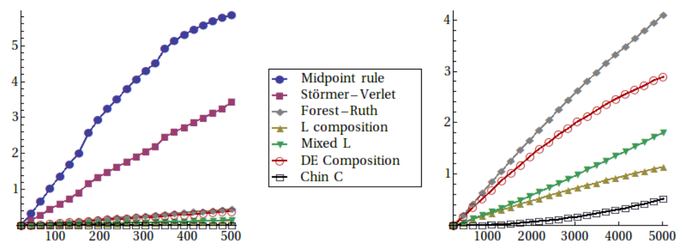
The precession rate is not as closely related to the total error as one might expect. In many cases the numerical solution has a phase shift which contributes significantly to the total error. For the composition methods LC and DEC this phase shift is highly dependent on the step size and the initial conditions. Hence the total error growth for these methods is also sensitive to the choice of step size and initial conditions. This can be seen by comparing Figure 4 and Figure 5.

To give a rough comparison of the computational effort required for the different methods, we list the running times of a long time calculation (20 000 steps):

We made a limited effort towards optimizing our implementation, so the given running times should only be taken as a rough indication. As expected the explicit methods SV, FR, and C are the fastest. For the composition methods DEC and LC only one out of every three steps is implicit, hence they are significantly faster than MP and ML.