Local cluster-size statistics in the critical phase of bond percolation on the Cayley tree

Tomoaki Nogawa Takehisa Hasegawa Koji Nemoto Email: nogawa@med.toho-u.ac.jp, takehisa.hasegawa.sci@vc.ibaraki.ac.jp and nemoto@statphys.sci.hokudai.ac.jp Affiliation: Department of Physics, Hokkaido University, Kita 10 Nishi 8, Kita-ku, Sapporo, Hokkaido, 060-0810, Japan

Abstract

We study bond percolation of the Cayley tree (CT) by focusing on the probability distribution function (PDF) of a local variable, namely, the size of the cluster including a selected vertex. Because the CT does not have a dominant bulk region, which is free from the boundary effect, even in the large-size limit, the phase of the system on it is not well defined. We herein show that local observation is useful to define the phase of such a system in association with the well-defined phase of the system on the Bethe lattice, that is, an infinite regular tree without boundary. Above the percolation threshold, the PDFs of the vertex at the center of the CT (the origin) and of the vertices near the boundary of the CT (the leaves) have different forms, which are also dissimilar to the PDF observed in the ordinary percolating phase of a Euclidean lattice. The PDF for the origin of the CT is bimodal: a decaying exponential function and a system-size-dependent asymmetric peak, which obeys a finite-size-scaling law with a fractal exponent. These modes are respectively related to the PDFs of the finite and infinite clusters in the nonuniqueness phase of the Bethe lattice. On the other hand, the PDF for the leaf of the CT is a decaying power function. This is similar to the PDF observed at a critical point of a Euclidean lattice but is attributed to the nesting structure of the CT around the boundary.

February 2014

Keywords: Classical phase transitions (Theory), Percolation problems (Theory), Random graphs, networks

1 Introduction

In recent years, statistical physics on complex networks [1] has been intensively developed [2]. Some collective phenomena on complex networks, such as percolation and the Ising model, show specific behaviors that are not observed in the systems on Euclidean lattices. For instance, a system exhibits behaviors similar to those observed in a system at a critical point, such as divergence of the susceptibility, in a finite range of the model parameter [3], which we call a critical phase. This type of critical region has been observed in percolation and the Ising model on Cayley trees (CTs) [3], hierarchical small-world networks [4, 5], and growing random networks [6]. On the basis of the renormalization group analysis of the systems on hierarchical small-world networks [7, 8], we speculate that small-world, i.e., infinite dimensional, and hierarchical properties of graphs play essential roles.

On inhomogeneous graphs in which vertices are not transitive, it is not trivial whether a phase of systems with large degrees of freedom can be defined by using macroscopic state variables in the same manner for systems on homogeneous graphs, e.g., Euclidean lattices. In the first place, we say that a system is in a single phase when the property of the system is homogeneous; if we divide a system into multiple macroscopic pieces of the same size, all pieces take the same value of extensive variables such as magnetization. In equilibrium, we suppose that the macroscopic state and the phase of a system are uniquely identified by a small number of extensive variables that is far fewer than the total degrees of freedom. It is natural to consider that the feasibility of the reduction in degrees of freedom is to a large extent dependent on the homogeneity. On the other hand, general inhomogeneous graphs cannot be divided into equal pieces, even in the macroscopic scale. Therefore we need further information other than extensive variables to describe systems on an inhomogeneous graph. On hierarchical graphs, small number of vertices often have a dominant influence on the state of the system. Furthermore local variables on such vertices probably behave quite differently from extensive variables, which are usually defined as summations of local variables without weighting. To adequately characterize the state of an inhomogeneous system, it is useful to observe local variables at representative vertices.

In this paper, we consider percolation on a CT to study the statistics of local variables. A CT is a subgraph of a Bethe lattice (BL), which is an infinite regular graph without cyclic path; an $n$ -layer CT is an $(n-1)$ -ball centered at a vertex of a BL. The boundary of a CT is given by leaves: the vertices with degree 1 in the outermost layer. The number fraction of the leaves remains positive for $n\to\infty$ , and therefore a CT does not have a dominant bulk region free from the boundary effect even in the limit $n\to\infty$ [9]. This is in contrast with the finite $d$ -dimensional Euclidean lattice, where the boundary is $(d-1)$ -dimensional and its fraction goes to zero in the large-size limit. The existence of the boundary brings inhomogeneity to a CT. When we consider the shortest paths between vertices, a few vertices near the origin are frequently used. Therefore the betweenness centrality is smaller for vertices in more outer layers; more important vertices have smaller populations. Inhomogeneity has an influence on the type of phase transition; whereas the Ising model on a BL undergoes a second-order transition [10, 11, 12], that on a CT undergoes an infinite-order transition [13, 14, 15]. Similar behavior is observed in the bond-percolation transitions on a CT and a BL [3], which will be reported in detail in the following sections. We also note that the continuous transition on a BL is known to be similar to those in the mean-field universality class, but its supercritical phase is not an ordinary percolating phase; an infinite cluster is not unique, but the number of infinite clusters is infinite [16, 17]. Such a phase is called a nonuniqueness phase [18]. For percolation on a CT, the same parameter region is a critical phase [3], where the cluster size histogram exhibits a power-law distribution. This paper aims to understand the critical phase of an inhomogeneous graph, a CT, in association with the nonuniqueness phase of a homogeneous graph, a BL. For this purpose, we investigate the probability distribution function (PDF) of the size of a locally-defined cluster and its moment for percolation on a CT. We show that the PDF of the vertices in the outer layers in the supercritical phase is similar to that observed at critical points of homogeneous systems. On the other hand, the PDFs of the vertices near the origin converge to that for a BL in the large-size limit, but an unignorable finite-size effect, which is related to an infinite number of infinite clusters, causes another kind of singular behavior for the moments. We propose two distinct finite-size-scaling laws for PDFs with respect to the two regimes.

2 Preliminary

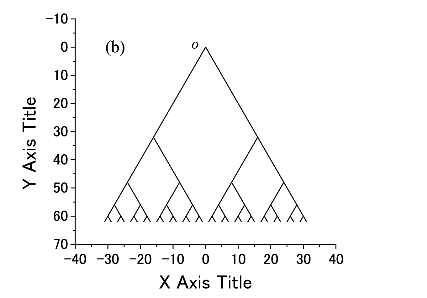
Refer to caption — Figure 1: (a) Cayley tree $\hat{T}_{7}$ (b) binary tree $T_{6}$ .

2.1 trees

Let $\hat{T}=(\hat{V},\hat{E})$ be the BL where the degree of every vertex is three. Here $\hat{V}$ and $\hat{E}$ denote the set of vertices and the set of edges, respectively. We arbitrarily choose a vertex ${\hat{o}}\in\hat{V}$ as the origin of $\hat{T}$ .

Let $\hat{T}_{n}=(\hat{V}_{n},\hat{E}_{n})$ be the CT with $n$ layers, that is an $(n-1)$ -ball in $\hat{T}$ centered at ${\hat{o}}$ . Figure 1(a) shows $\hat{T}_{7}$ . We say that $v\in\hat{T}_{n}$ is in the $l$ th layer when $d({\hat{o}},v)$ : the shortest path length between ${\hat{o}}$ and $v$ equals $l\in\{0,1,\cdots,n-1\}$ . We call the vertices in the $(n-1)$ th layer leaves, whose degrees are unity. The numbers of the vertices and the edges are $|\hat{V}_{n}|=3\times 2^{n-1}-2$ and $|\hat{E}_{n}|=|\hat{V}_{n}|-1$ , respectively.

By removing ${\hat{o}}$ and three edges connecting to it from $\hat{T}$ , we obtain three infinite binary trees. Let $T=(V,E)$ denote one of them. We denote by $o$ the vertex that once connected to ${\hat{o}}$ and call it the root. Let $T_{n}=(V_{n},E_{n})$ be the binary tree with $n$ layers, that is an $(n-1)$ -ball in $T$ centered at $o$ . Figure 1(b) shows $T_{6}$ . We define the layers of $T_{n}$ similarly for $\hat{T}_{n}$ , and then the vertices in the $(n-1)$ th layers are leaves. The numbers of the vertices and the edges are $|V_{n}|=2^{n}-1$ and $|E_{n}|=|V_{n}|-1$ , respectively. Hereafter, we assume $|V_{n}|\gg 1$ , and then approximate $|V_{n}|$ by $2^{n}$ .

2.2 percolation

Let us consider bond percolation for $T_{n}$ . Each $e\in E_{n}$ is independently open with a unique probability $p$ and closed with probability $1-p\equiv\overline{p}$ . The connected components of the open edges are called clusters. We denote the set of vertices in the cluster including $v\in V_{n}$ by $C_{nv}(\subseteq V_{n})$ and denote the cluster size, that is the number of vertices in $C_{nv}$ , by $|C_{nv}|$ . We also consider bond percolation for $\hat{T}_{n}$ , $T$ , and $\hat{T}$ . Then, we similarly define $\hat{C}_{nv}$ for $\hat{T}_{n}$ , $C_{v}$ for $T$ and $\hat{C}_{v}$ for $\hat{T}$ .

2.3 probability distribution functions (PDFs) of cluster sizes

Here we introduce some PDFs of cluster sizes. For $v\in T_{n}$ , we define

\displaystyle q_{nv}(s)\equiv P(|C_{nv}|=s)=\left\langle\delta_{s|C_{nv}|}\right\rangle.

(1)

Hereafter, $P(X)$ is the probability of a proposition $X$ , which is a function of $p$ (but we omit to note) and $\langle x\rangle$ is the expectation value of $x$ . Similarly, we define $\hat{q}_{nv}(s)\equiv P(|\hat{C}_{nv}|=s)$ for $\hat{T}_{n}$ . For $\hat{T}$ , we define a unique PDF $\hat{q}(s)\equiv P(|C_{\hat{o}}|=s)$ because $P(|C_{v}|=s)$ does not depend on $v$ . Similarly, we define $q(s)\equiv P(|C_{o}|=s)$ for $T$ .

Remembering that $T_{n}\subset T$ , we have

	$\displaystyle q_{no}(s)$	$\displaystyle=$	$\displaystyle P\left(\|C_{o}\cap V_{n}\|=s\right)$		(2)
		$\displaystyle=$	$\displaystyle P\left(C_{o}\subseteq V_{n}\wedge\|C_{o}\|=s\right)+P\left(C_{o}\not\subseteq V_{n}\wedge\|C_{o}\cap V_{n}\|=s\right).$		(2)

From the fact that $|C_{o}\cap V_{n}|\leq n-1\Rightarrow C_{o}\subset V_{n}$ , we have

\displaystyle q_{no}(s)=q(s)\ \ \mathrm{for}\ \ s\leq n-1\quad\Rightarrow\quad\lim_{n\to\infty}q_{no}(s)=q(s)\ \ \mathrm{for}\ \ s<\infty.

(3)

In a similar way, we have $\lim_{n\to\infty}\hat{q}_{n{\hat{o}}}(s)=\hat{q}(s)$ . Furthermore, we have $\lim_{n\to\infty}\hat{q}_{nv}(s)=\hat{q}(s)$ if $d({\hat{o}},v)<\infty$ . Note that similar relation does not hold for $q_{nv}$ unless $v=o$ .

2.4 local fractal exponent

To quantify the upper cutoff of the PDF, we define a local fractal exponent for $v\in V_{n}$ as

\displaystyle\psi_{v}\equiv\inf\left\{\varphi\ {\big|}\ \varphi>0,\ \lim_{n\to\infty}P\left(|C_{nv}|>|V_{n}|^{\varphi}\right)=0\right\}.

(4)

Similarly we define $\hat{\psi}_{v}$ for $v\in\hat{V}_{n}$ . For percolation on an Euclidean lattice, this exponent equals zero in a nonpercolating phase and unity in a percolating phase. In the former, the PDF of a cluster size decays exponentially. In the latter, the PDF has a Gaussian peak whose position is asymptotically proportional to the number of total vertices. This peak is related to a unique giant component for each sample.

2.5 moments

We define the $m$ -th order moment of $q_{nv}(s)$ for $T_{n}$ as

\displaystyle\chi_{nv}^{(m)}\equiv\langle|C_{nv}|^{m}\rangle=\sum_{s=1}^{\infty}s^{m}q_{nv}(s).

(5)

Similarly, we define $\hat{\chi}_{nv}^{(m)}$ for $\hat{q}_{nv}(s)$ , $\chi^{(m)}$ for $q(s)$ and $\hat{\chi}^{(m)}$ for $\hat{q}(s)$ . Note that $\chi^{(m)}$ and $\hat{\chi}^{(m)}$ does not include the contribution from infinite clusters and therefore does not necessarily diverge even if an infinite cluster exists with positive probability.

2.6 Generating functions (GFs)

We define the GF for $q_{nv}$ as

\displaystyle Q_{nv}(x)\equiv\sum_{s=1}^{\infty}q_{nv}(s)x^{s}.

(6)

The moments of a PDF is calculated by differentiating the corresponding GF, e.g.,

\displaystyle\chi_{nv}^{(m)}=Q_{nv}^{(m)}(1)\equiv\left.\left(x\frac{d}{dx}\right)^{\!\!m}\!Q_{nv}(x)\right|_{x=1}.

(7)

Similarly, we define $\hat{Q}_{nv}(x)$ for $\hat{q}_{nv}(s)$ , $Q(x)$ for $q(s)$ and $\hat{Q}(x)$ for $\hat{q}(s)$ .

From the nesting structure of $T_{n}$ , we have a recursion equation for $Q_{no}(x)$ as

\displaystyle Q_{n+1,o}(x)=x[pQ_{no}(x)+\overline{p}]^{2}.

(8)

With $Q_{no}(x)$ , the recursion equation for $Q_{no}(x)$ is given by

\displaystyle\hat{Q}_{n+1,o}(x)=x[pQ_{no}(x)+\overline{p}]^{3}=Q_{n+1,o}(x)[pQ_{no}(x)+\overline{p}].

(9)

3 Results

In this section, we investigate the PDF and the singularities of the moments, which are related to the analyticity of GFs as a function of $p$ and $x$ . We focus on the results for $T_{n}$ and $T$ , but their properties are almost the same with those for $\hat{T}_{n}$ and $\hat{T}$ , respectively.

3.1 Infinite trees

First we overview the results for the infinite binary tree, $T$ [19, 20]. From Eq. (3), we have $Q(x)=\lim_{n\to\infty}Q_{n}(x)$ . By evaluating the fixed point of Eq. (8), we obtain

	$\displaystyle Q(x)=\frac{1-2p\overline{p}x-\sqrt{1-4p\overline{p}x}}{2p^{2}x},\quad Q^{(1)}(x)=\frac{x[\overline{p}+pQ(x)]^{2}}{1-2px[\overline{p}+pQ(x)]},$		(10)
	$\displaystyle q(s)\propto s^{-3/2}(4p\overline{p})^{s}\quad\mathrm{for}\quad s\gg 1.$		(11)

See A.1 and A.2 for the derivation. The transition threshold is given by $p=p_{c}=1/2$ , at which $4p\overline{p}$ equals unity and then the exponential cutoff of $q(s)$ diverges.

From the second equation of Eq. (10), the probability that $o$ is included in a finite cluster is given by

\displaystyle Q(1)=\sum_{s=1}^{\infty}q(s)=\frac{2p^{2}+(1-2p)-|1-2p|}{2p^{2}}=\left\{\begin{array}[]{ccc}1&\mathrm{for}&p\leq p_{c}\\ (\overline{p}/p)^{2}&\mathrm{for}&p>p_{c}\end{array}\right..

Thus, the probability that $o$ is included in an infinite cluster is given by

\displaystyle P_{\infty}\equiv 1-Q(1)=\left\{\begin{array}[]{ccc}0&\mathrm{for}&p\leq p_{c}\\ 1-(\overline{p}/p)^{2}&\mathrm{for}&p>p_{c}\end{array}\right..

For $p\searrow p_{c}$ , we have a power law

\displaystyle P_{\infty}\propto(p-p_{c})^{\beta},\quad\beta=1.

(18)

From Eq. (10) and Eq. (3.1), we have

\displaystyle\chi^{(1)}=Q^{(1)}(1)=\left\{\begin{array}[]{ccc}\displaystyle\frac{1}{1-2p}&\mathrm{for}&p<p_{c}\\ \displaystyle\left(\frac{\overline{p}}{p}\right)^{2}\frac{1}{2p-1}&\mathrm{for}&p>p_{c}\end{array}\right..

In the limits $p\nearrow p_{c}$ and $p\searrow p_{c}$ , $\chi^{(1)}$ diverges and a power-law

\displaystyle\chi^{(1)}\propto|p-p_{c}|^{-\gamma},\quad\gamma=1,

(22)

holds. The higher moment, $\chi^{(m)}$ with $m>1$ , is also finite for $p\neq p_{c}$ because $q(s)$ decays exponentially with increasing $s$ for $p\neq p_{c}$ .

For $\hat{T}_{n}$ , we have

	$\displaystyle\hat{P}_{\infty}\equiv 1-\hat{Q}(1)=\left\{\begin{array}[]{ccc}0&\mathrm{for}&p\leq p_{c}\\ 1-(\overline{p}/p)^{3}&\mathrm{for}&p>p_{c}\end{array}\right.,$
	$\displaystyle\hat{\chi}^{(1)}=\left\{\begin{array}[]{ccc}\displaystyle\frac{1+p}{1-2p}&\mathrm{for}&p<p_{c}\\ \displaystyle\left(\frac{\overline{p}}{p}\right)^{3}\frac{2-p}{2p-1}&\mathrm{for}&p>p_{c}\end{array}\right..$

Power-laws same as Eq. (18) and Eq. (22) hold for $\hat{P}_{\infty}$ and $\hat{\chi}^{(1)}$ , respectively.

3.2 Root

Here we consider the PDF for the cluster including the root of the finite binary tree.

3.2.1 PDF

As mentioned before, $q_{no}(s)$ converges to $q(s)$ for $n\to\infty$ . For $p<p_{c}$ , $q_{no}(s)$ is very similar to $q(s)$ except the existence of the finite size cutoff. For $p>p_{c}$ , $q_{no}(s)$ has characteristic bimodal structure as indicated in Fig. 2(a). The separation of the two modes becomes clearer as $n$ increases. The small- $s$ part converges to $q(s)$ for $n\to\infty$ . On the other hand, the large- $s$ part forms an asymmetric peak, whose position moves to the larger $s$ direction and the height decreases toward zero with increasing $n$ . Let us denote the large- $s$ part by

\displaystyle q^{>}_{no}(s)\equiv q_{no}(s)-q(s).

(29)

Whereas $q(s)$ corresponds to the part of finite clusters for the PDF in $T$ , $q^{>}_{no}(s)$ is related to the statistical property of an infinite cluster in $T$ ; for large $s$ such that $q(s)\ll q_{no}(s)$ , $q_{no}(s)$ corresponds to the second term on the r.h.s. of Eq. (2) and we have

\displaystyle q^{>}_{no}(s)\approx P\left(|C_{o}|=\infty\wedge|C_{o}\cap V_{n}|=s\right).

(30)

We remark that $\sum_{s=1}^{\infty}q^{>}_{no}(s)=P_{\infty}$ and $q^{>}_{no}(s)=0$ for $s\leq n-1$ .

Figure 2(a) indicates that the shape of $q^{>}_{no}(s)$ ’s for various $n$ are congruent in the double-logarithmic plot. We assume that $q^{>}_{no}(s)$ asymptotically obeys a power-law:

\displaystyle q^{>}_{no}(s)=|V_{n}|^{-\psi}\tilde{q}^{>}(s|V_{n}|^{-\psi})=s^{-1}\tilde{\tilde{q}}^{>}(s|V_{n}|^{-\psi})

(31)

for $s\gg 1$ . Here $\tilde{q}^{>}(x)$ is a scaling function and $\tilde{\tilde{q}}^{>}(x)\equiv x\tilde{q}^{>}(x)$ . As to the scaling exponent $\psi$ , we will show

\displaystyle\psi=\log_{2}(2p)

(32)

in Sec. 3.2.3. The exponent $\psi$ monotonically increases from 0 to 1 as $p$ increases from $p_{c}$ to 1. Numerical result in Fig. 2(b) supports our scaling assumption. Moreover, the scaling function is a power function as

\displaystyle\tilde{q}^{>}(x)\propto x^{\tau^{\prime}}\ \ \mathrm{for}\ \ x\ll 1,\quad\tau^{\prime}=-\frac{\ln 2\overline{p}}{\ln 2p}-1.

(33)

(The evaluation of $\tau^{\prime}$ is shown in A.3.) The exponent $\tau^{\prime}$ equals zero at $p=p_{c}$ and monotonically increases with $p$ to diverge for $p\to 1$ .

3.2.2 local fractal exponent

By using Eq. (31), we have

\displaystyle P(|C_{no}|>|V_{n}|^{\varphi})\approx\int_{|V_{n}|^{\varphi}}^{\infty}ds|V_{n}|^{-\psi}\tilde{q}^{>}(s|V_{n}|^{-\psi})=\int_{|V_{n}|^{\varphi-\psi}}^{\infty}dx\tilde{q}^{>}(x).

(34)

In the first equation, we omit the contribution from $q(s)$ . In the limit $n\to\infty$ , this goes to zero for $\varphi>\psi$ and converges to a positive constant, that is, $P_{\infty}$ for $\varphi<\psi$ . Thus, we have

\displaystyle\psi_{o}=\psi.

(35)

3.2.3 moments

Next, we consider the asymptotic behavior of $\chi_{no}^{(m)}$ for $p>p_{c}$ and $n\to\infty$ . From Eq. (31), we have

	$\displaystyle\chi_{no}^{(m)}$	$\displaystyle\approx$	$\displaystyle\chi^{(m)}+\int_{1}^{\infty}dss^{m}\|V_{n}\|^{-\psi}\tilde{q}^{>}(s\|V_{n}\|^{-\psi})$		(36)
		$\displaystyle\approx$	$\displaystyle\|V_{n}\|^{m\psi}\int_{\|V_{n}\|^{-\psi}}^{\infty}dxx^{m}\tilde{q}^{>}(x)\propto\|V_{n}\|^{m\psi}$		(36)

for $n\to\infty$ . In the second approximation, we ignored $\chi^{(m)}$ , which is finite for $n\to\infty$ . Consequently, $\chi_{no}^{(m)}$ with arbitrary $m>0$ diverges in the limit $n\to\infty$ for $p>p_{c}$ .

For $m=1$ , we can exactly calculate $\chi_{no}^{(1)}=\langle|C_{no}|\rangle$ and estimate $\psi$ by comparing its asymptotic form and Eq. (36). We have $P(v\in C_{no})=p^{d(o,v)}$ , which leads to

\displaystyle\chi_{no}^{(1)}=\left\langle\sum_{v\in C_{no}}1\right\rangle=\sum_{v\in V_{n}}P(v\in C_{no})=\sum_{l=0}^{n-1}2^{l}p^{l}=\frac{(2p)^{n}-1}{2p-1}

(37)

for $p\neq p_{c}$ . (At $p=p_{c}$ , $\chi_{no}^{(1)}$ equals $n\approx\log_{2}|V_{n}|$ .) For $p>p_{c}$ and $n\to\infty$ , $\chi_{no}^{(1)}$ is proportional to $(2p)^{n}\propto|V_{n}|^{\log_{2}(2p)}$ . Thus we have Eq. (32).

3.3 Leaf

Let $v_{l}$ be a vertex distant from the outermost layer by $l$ , i.e., in the $(n-l-1)$ th layer of $T_{n}$ . In this subsection, we consider the limit $n\to\infty$ with fixing $l$ .

3.3.1 PDF

We plot $q_{nv_{l}}(s)$ for $p=0.8>p_{c}$ with several values of $l$ in Fig. 3(a) and of $n$ in Fig. 3(b). When $1\ll|V_{l}|^{\psi}\ll|V_{n}|^{\psi}$ , we observe four regimes;

\displaystyle q_{nv_{l}}(s)\left\{\begin{array}[]{lcl}=\hat{q}(s)&\mathrm{for}&s\leq l\\ \propto s^{\tau^{\prime}}&\mathrm{for}&1\ll s\ll|V_{l}|^{\psi}\\ \propto s^{-1/\psi}&\mathrm{for}&|V_{l}|^{\psi}\ll s\ll|V_{n}|^{\psi}\\ \mathrm{rapid\ decay}&\mathrm{for}&s\gg|V_{n}|^{\psi}\end{array}\right..

The second crossover from power-law growth to power-law decay occurs when $C_{nv_{l}}$ begins to reach the nearest leaves, which are distant from $v_{l}$ by $l$ , probably. In this crossover, $q_{nv_{l}}(s)$ obeys the scaling law obtained by replacing $|V_{n}|$ in Eq. (31) with $|V_{l}|$ as shown in Fig. 3(c). The origin of the power-law decay is roughly understood as follows. By letting $q_{nv_{l}}(j|s)$ be the PDF under the condition that the upper end of $C_{nv_{l}}$ is $v_{j-1}$ and approximating $q_{nv_{l}}(j|s)$ by $q_{jo}(s)$ , we have

	$\displaystyle q_{nv_{l}}(s)$	$\displaystyle=$	$\displaystyle\sum_{j=l+1}^{n-1}\overline{p}p^{j-l-1}q_{nv_{l}}(j\|s)+p^{n-l-1}q_{nv_{l}}(n\|s)$		(43)
		$\displaystyle\approx$	$\displaystyle\frac{\overline{p}}{p^{l+1}}\sum_{j=-\infty}^{\infty}p^{j}q_{jo}(s)\approx\frac{\overline{p}}{p^{l+1}}\sum_{j=-\infty}^{\infty}\|V_{j}\|^{-1}\tilde{q}^{>}(s\|V_{j}\|^{-\psi}).$		(43)

In the second equation (approximation), we assume $|V_{l}|^{\psi}\ll s\ll|V_{n}|^{\psi}$ and modify the lower and upper bounds of the series by using that the series is dominated by the terms with $j$ such that $|V_{j}|^{\psi}\sim s$ . For the same reason, we ignore the term, $p^{n-l-1}q_{nv_{l}}(n|s)$ . In the last equation, we ignore the component $q(s)$ in $q_{j+1,o}(s)$ and use the scaling law, Eq. (31), and $p^{j}=2^{(\psi-1)j}\approx|V_{j}|^{\psi-1}$ . Equation (43) satisfies $q_{nv_{l}}(2^{-\psi}s)=2q_{nv_{l}}(s)$ , which leads to $q_{nv_{l}}(s)\propto s^{-1/\psi}$ . More accurate calculation is shown in B.

The third crossover around $s\sim|V_{n}|^{\psi}$ obeys another scaling law:

\displaystyle q_{nv_{l}}(s)=|V_{n}|^{-1}\tilde{q}_{l}(s|V_{n}|^{-\psi})=s^{-1/\psi}\tilde{\tilde{q}}_{l}(s|V_{n}|^{-\psi})\quad\mathrm{for}\quad s\gg|V_{l}|^{\psi},

(44)

as shown in Fig. 3(d). This is derived from Eq. (31) and $\lim_{x\to 0}\tilde{\tilde{q}}_{l}(x)$ is a finite constant (See B).

3.3.2 local fractal exponent

As shown in the Sec. 3.3.1, the large- $s$ behavior is governed by the power-law decay. By using Eq. (44), we have

	$\displaystyle P(\|C_{nv_{l}}\|>\|V_{n}\|^{\varphi})$	$\displaystyle\approx$	$\displaystyle\int_{\|V_{n}\|^{\varphi}}^{\infty}dss^{-1/\psi}\tilde{\tilde{q}}_{l}(s\|V_{n}\|^{-\psi})$		(45)
		$\displaystyle=$	$\displaystyle\|V_{n}\|^{\psi-1}\int_{\|V_{n}\|^{\varphi-\psi}}^{\infty}dxx^{-1/\psi}\tilde{\tilde{q}}_{l}(x).$		(45)

For $\varphi>\psi$ , both the integral and the prefactor goes to zero. For $\varphi\in(0,\psi]$ , we have to care about the infrared divergence as

\displaystyle P(|C_{nv_{l}}|>|V_{n}|^{\varphi})\approx|V_{n}|^{\psi-1}|V_{n}|^{(\varphi-\psi)(1-1/\psi)}\tilde{\tilde{q}}_{l}(0)=|V_{n}|^{-(1/\psi-1)\varphi}\tilde{\tilde{q}}_{l}(0),

(46)

which vanishes for $n\to\infty$ for $\psi<1$ . Thus, we have

\displaystyle\psi_{v_{l}}=0\quad\iff\quad\lim_{n\to\infty}P(|C_{nv_{l}}|<\infty)=1\quad\mathrm{for}\ p<1\ \mathrm{and}\ l<\infty.

(47)

The local exponents for vertices near the leaves do not coincide with $\psi$ appearing in the scaling equation (44), unlike that for vertices near the root.

3.3.3 moments

By using Eq. (44), we have

\displaystyle\chi_{nv_{l}}^{(m)}\approx\int_{1}^{\infty}dss^{m}s^{-1/\psi}\tilde{\tilde{q}}_{l}(s|V_{n}|^{-\psi})=|V_{n}|^{\psi^{(m)}}\int_{|V_{n}|^{-\psi}}^{\infty}dxx^{\psi^{(m)}\!/\psi-1}\tilde{\tilde{q}}_{l}(x),

(48)

where $\psi^{(m)}\equiv(m+1)\psi-1.$ When

\displaystyle\psi^{(m)}>0\ \iff\ p>p_{c}^{(m)}\equiv 2^{-m/(1+m)},

(49)

the integral in the most r.h.s. of Eq. (48) converges to a finite value for $n\to\infty$ . Thus $\chi_{nv_{l}}^{(m)}$ diverges being proportional to $|V_{n}|^{\psi^{(m)}}$ for $p>p_{c}^{(m)}$ . For $p<p_{c}^{(m)}$ , the integral in the infrared region is dominant and it converges to $\tilde{\tilde{q}}_{l}(0)\psi/|\psi^{(m)}|\propto(p_{c}^{(m)}-p)^{-1}$ for $n\to\infty$ . For $p=p_{c}^{(m)}$ , $\chi_{nv_{l}}^{(m)}$ logarithmically diverges with increasing $n$ . Thus we have

\displaystyle\chi_{nv_{l}}^{(m)}\propto\left\{\begin{array}[]{ccc}(p_{c}^{(m)}-p)^{-1}&\mathrm{for}&p\nearrow p_{c}^{(m)}\\ \ln|V_{n}|&\mathrm{for}&p=p_{c}^{(m)}\\ |V_{n}|^{\psi^{(m)}}&\mathrm{for}&p>p_{c}^{(m)}\end{array}\right.

for $n\to\infty$ . Note that

\displaystyle 1>p_{c}^{(1)}>p_{c}^{(2)}>\cdots>\lim_{m\to\infty}p_{c}^{(m)}=p_{c}.

(54)

Thus only the infinite-order moment diverges at $p=p_{c}$ . This type of weak singularity at $p_{c}$ is called an infinite-order transition. As $p$ increases, the lowest order of the diverging moments decreases.

4 summary and discussions

In this paper, we investigated the PDF for a local variable of the CT, namely, the size of the cluster including a selected vertex, especially, the origin and a leaf. (Although we mainly calculate $q_{nv}(s)$ for the binary tree, we remark that $\hat{q}_{nv}(s)$ for the CT is essentially same with $q_{nv}(s)$ except unimportant constant factor and the shape of the cutoff of the scaling functions.) We found that the PDF for the origin converges to that for BL and that for the leaves converges to a power-law function. These behaviors are respectively similar to that in a percolating phase and that at a critical point in Euclidean systems. Regarding finite size effects, the former has an asymmetric peak with a long tail toward the smaller size direction, whereas the latter exhibits a simple cutoff. These obey their own scaling laws. By using the scaling laws, we showed that the local fractal exponent for the origin is positive and that for the leaves is zero. These properties correspond to the fact that the probability that the vertex belongs to an infinite cluster is positive and zero, respectively. In addition, any positive-order moment of the local cluster size for the origin diverges. For the leaves, only the infinite-order moment diverges at the critical point and the lower-order moments diverge stepwise as $p$ increases.

The power-law of the PDF for the leaves leads to the power-law of the global distribution function, that is, the cluster size histogram per vertex;

\displaystyle n_{s}\equiv\left\langle\frac{1}{|\hat{V}_{n}|}\sum_{v\in\hat{V}_{n}}\frac{\delta_{s|\hat{C}_{nv}|}}{|\hat{C}_{nv}|}\right\rangle=\frac{1}{|\hat{V}_{n}|}\sum_{v\in\hat{V}_{n}}\frac{\hat{q}_{nv}(s)}{s}\propto s^{-\tau}.

(55)

Since the contribution to the summation is dominated by leaves, we have $n_{s}\approx s^{-1}\hat{q}_{nv_{o}}(s)$ and therefore $\tau=1+1/\psi$ . A similar power-law is observed at the critical point of an ordinary second-order transition in Euclidean lattices. However, we should note that the power-law of Euclidean systems is observed also in the local PDF for the bulk region free from the boundary effect whereas the power-law directly reflects the boundary effect and the nesting structure of the graph itself in the case of the CT. The power-law at a critical point of a finite-dimensional system represents the quasi-long-range coherence, i.e., power-law decay of connectedness via open bonds, due to the divergence of a characteristic length. In the critical phase of the CT, the connectedness between two vertices has short-range coherence decaying exponentially as $p^{d(o,v)}$ .

Whereas the PDF for the leaves strongly reflects the boundary effect, the PDF for the origin is related to that for the vertices in the BL. Thus, the observation of the latter enables us to argue the phase of the system in the same framework with the infinite homogeneous system, where the phase is well defined. When we consider only finite clusters on the BL, the PDF is an exponential function as well as in the ordinary percolating phase. However, the peak due to finite-size effect, $q_{n}^{>}(s)$ , is significantly different. This component can be identified with the PDF of the size of the intersection between an infinite cluster on the BL and an $(n-1)$ -ball centered at the origin. If the supercritical phase was the ordinary percolating phase and there exists a unique infinite cluster, the PDF would have a Gaussian peak centered at $s\approx\hat{P}_{\infty}|\hat{V}_{n}|$ . Actually, the PDF has an asymmetric peak whose center position is $O(|\hat{V}_{n}|^{\psi})$ with $\psi\in(0,1)$ .

In the percolating phase of a homogeneous system, an infinite cluster is unique and then we have

\displaystyle\hat{P}_{\infty}\equiv\lim_{\varphi\searrow 0}\lim_{n\to\infty}P(|\hat{C}_{n{\hat{o}}}|>|\hat{V}_{n}|^{\varphi})=m\equiv\sqrt{\lim_{n\to\infty}\langle|\hat{C}_{n{\hat{o}}}|\rangle/|\hat{V}_{n}|}.

(56)

Here $\hat{P}_{\infty}$ and $m$ are local quantities. This equation does not hold in the critical phase; $\hat{P}_{\infty}$ is positive but $m$ equals zero since $\langle|\hat{C}_{n{\hat{o}}}|\rangle\propto|\hat{V}_{n}|^{\psi}$ . Note that $\hat{P}_{\infty}$ is the probability that $\hat{C}_{o}$ in the BL is not finite and therefore tells us nothing about the number of infinite clusters. We have to distinguish these order parameters. We propose to call $m$ an extensive order parameter, which is zero in the critical phase and positive in the percolating phase, and call $\hat{P}_{\infty}$ subextensive order parameters, which are positive in both phases. We remark that $\hat{P}_{\infty}>0\iff\psi_{o}>0$ and $m>0\iff\psi_{o}=1$ .

We expect all properties described in this paper to apply to percolation on infinite nonamenable graphs (NAGs) and the asymptotic limit of the increasing sequence of their subgraph. NAGs include BLs, enhanced trees [21, 22] and hyperbolic lattices [23]. It has been proved that there exists a phase where an infinite number of infinite clusters exist in the percolation on NAGs [24, 23]. In addition, we have preliminarily confirmed that a similar result appears in percolation on a hierarchical small-world network, namely, the Faray graph [5, 8], which exhibits a critical phase and a percolating phase. Note that the Faray graph is defined as an increasing sequence of a graph and cannot be regarded as a subgraph of a well-defined, infinite inhomogeneous graph unlike a CT. In the critical phase, the PDF for the vertex with the largest degree is similar to the $\hat{q}_{no}(s)$ , although the exponent $\tau^{\prime}$ is negative. In addition, the cluster-size histogram is a decaying power function as Eq. (55). Therefore, we expect that it is possible to link the critical phase of the intrinsically inhomogeneous systems to the well-defined nonuniqueness phase on infinite homogeneous NAGs, via the property of local variables. To confirm the generality of this idea, we need to research the local PDF for various graphs where the cluster-size histograms obey the power-law.

TH is grateful for the financial support from the Grant-in-Aid for Young Scientists (B) (Grant No. 15K17716), Grant-in-Aid for Scientific Research (B) (Grant No. 26310203), and JST, ERATO, Kawarabayashi Large Graph Project.

Appendix A Calculation of the PDF for the root vertex

A.1 recursion equation and fixed point

By using the fact that $T_{n+1}$ includes two $T_{n}$ ’s, we obtain a recursion equation:

\displaystyle Q_{n+1,o}(x)=x[\overline{p}+pQ_{no}(x)]^{2}.

(57)

The fixed point of this recursion equation, $Q(x)$ , is given by

\displaystyle Q(x)=x[\overline{p}+pQ(x)]^{2}\quad\iff\quad Q(x)=\frac{1-2p\overline{p}x\pm\sqrt{1-4p\overline{p}x}}{2p^{2}x}.

(58)

The stable fixed point for the initial condition $Q_{1o}(x)=x$ is the one denoted by minus sign. By differentiating Eq. (57), we obtain the recursion equation of $Q^{(1)}_{no}(x)$ and its fixed point $Q^{(1)}(x)$ as

	$\displaystyle Q^{(1)}_{n+1,o}(x)$	$\displaystyle=$	$\displaystyle[\overline{p}+pQ_{no}(x)]\{x[\overline{p}+pQ_{no}(x)]+2pQ^{(1)}_{no}(x)\},$		(59)
	$\displaystyle Q^{(1)}(x)$	$\displaystyle=$	$\displaystyle\frac{x[\overline{p}+pQ(x)]^{2}}{1-2px[\overline{p}+pQ(x)]}.$		(60)

By substituting $Q_{no}(x)=\sum_{s=1}^{\infty}q_{no}(s)x^{s}$ into Eq.(57), we have

\displaystyle\sum_{s=1}^{\infty}q_{n+1,o}(s)x^{s}=\overline{p}^{2}x+x\sum_{s=1}^{\infty}\left[2p\overline{p}q_{no}(s)+p^{2}\sum_{t=1}^{s-1}q_{no}(t)q_{no}(s-t)\right]x^{s}.

(61)

By comparing the coefficients for each order of $x^{s}$ , we obtain a recursion equation for $s\geq 2$ as

\displaystyle q_{n+1,o}(s)=2p\overline{p}q_{no}(s-1)+p^{2}\sum_{t=1}^{s-2}q_{no}(t)q_{no}(s-1-t)

(62)

with an initial condition $q_{1o}(s)=\delta_{s1}$ and a boundary condition $q_{no}(1)=\overline{p}^{2}$ for $n\geq 2$ .

For $\hat{T}_{n}$ , we have the recursion equations and the fixed point as

$\displaystyle\hat{Q}_{n+1,o}(x)$	$\displaystyle=$	$\displaystyle x[\overline{p}+pQ_{no}(x)]^{3}=Q_{n+1,o}(x)[\overline{p}+pQ_{no}(x)],$	(63)
$\displaystyle\hat{q}_{n+1,o}(s)$	$\displaystyle=$	$\displaystyle\overline{p}q_{n+1,o}(s)+p\sum_{t=1}^{s-1}q_{n+1,o}(t)q_{no}(s-t),$	(64)
$\displaystyle\hat{Q}(x)$	$\displaystyle=$	$\displaystyle Q(x)[\overline{p}+pQ(x)],$	(65)
$\displaystyle\hat{q}(s)$	$\displaystyle=$	$\displaystyle\overline{p}q(s)+p\sum_{t=1}^{s-1}q(t)q(s-t).$	(66)

A.2 function form of $q(s)$

By using an equality

\displaystyle\sqrt{1-y}=1-\frac{y}{2}-\sum_{n=2}^{\infty}\frac{(2n-3)!}{n!(n-2)!}\frac{y^{n}}{2^{2n-2}}

(67)

in Eq. (58), we have

\displaystyle q(s)=2\,\frac{\overline{p}}{p}\frac{(2s-1)!}{(s+1)!(s-1)!}(p\overline{p})^{s}.

(68)

We remark that $p^{2}q(s)$ is a function of $p\overline{p}$ and is invariant against the replacement of $p$ with $\overline{p}$ , i.e., the reflection at $p=1/2$ . By multiplying the both sides of Eq. (66) by $p^{3}$ , we can show that $p^{3}\hat{q}(s)$ is also a function of $p\overline{p}$ .

Equation (68) leads to

\displaystyle\frac{q(s+1)}{q(s)}=\frac{s+1/2}{s+2}(4p\overline{p}).

(69)

For $p=1/2$ , we have $q(s+1)-q(s)=-[3/2(s+2)]q(s)$ . For $s\gg 1$ , we have

\displaystyle\frac{dq(s)}{ds}\approx-\frac{3}{2}\frac{q(s)}{s}\ \iff\ q(s)\propto s^{-3/2}.

(70)

For arbitrary $p$ and $s\gg 1$ , we have

\displaystyle q(s)=(4p\overline{p})^{s}q(s)\Big|_{p=p_{c}}\propto s^{-3/2}(4p\overline{p})^{s}.

(71)

A.3 evaluation of $\tau^{\prime}$

The deviation of the GF from the fixed point,

\displaystyle Q_{no}(x)-Q(x)\equiv Q_{no}^{>}(x)=\sum_{s=1}^{\infty}q_{no}^{>}(s)x^{s},

(72)

satisfies

$\displaystyle Q_{n+1,o}^{>}(x)$	$\displaystyle=$	$\displaystyle px\left\{2\overline{p}+p[2Q(x)+Q_{no}^{>}(x)]\right\}Q_{no}^{>}(x),$	(73)
$\displaystyle q_{n+1,o}^{>}\left(s\right)$	$\displaystyle=$	$\displaystyle 2p\overline{p}q_{no}^{>}(s-1)+2p^{2}\sum_{t=1}^{s-2}q(t)q_{no}^{>}(s-1-t)$	(74)
		$\displaystyle+p^{2}\sum_{t=1}^{s-2}q_{no}^{>}(t)q_{no}^{>}(s-1-t).$	(74)

By substituting $q_{no}^{>}(s)=|V_{n}|^{-\psi}\tilde{q}^{>}(s|V_{n}|^{-\psi})$ to Eq. (74), we obtain

	$\displaystyle\tilde{q}^{>}\left(sh^{-(n+1)}\right)$	$\displaystyle=$	$\displaystyle 2p\overline{p}h\tilde{q}^{>}\left((s-1)h^{-n}\right)+2p^{2}h\sum_{t=1}^{s-2}q(t)\tilde{q}^{>}\left((s-1-t)h^{-n}\right)$		(75)
			$\displaystyle+p^{2}h^{1-n}\sum_{t=1}^{s-2}\tilde{q}^{>}(th^{-n})\tilde{q}^{>}\left((s-1-t)h^{-n}\right).$		(75)

Here we put $h\equiv 2^{\psi}(=2p)$ and use $|V_{n}|^{\psi}\approx h^{n}$ . The third term on the r.h.s., which is less than $p^{2}h^{1-n}\sum_{t=1}^{s}\tilde{q}^{>}(sh^{-n})^{2}\propto p^{2}h(sh^{-n})^{1+2\tau^{\prime}}$ , is negligible for $s\ll h^{n}$ . By putting $sh^{-n}=x$ , we have

	$\displaystyle\tilde{q}^{>}(x/h)$	$\displaystyle\approx$	$\displaystyle 2p\overline{p}h\tilde{q}^{>}(x)+2p^{2}h\sum_{t=1}^{\infty}q(t)\tilde{q}^{>}\left(x-(1+t)h^{-n}\right)$		(76)
		$\displaystyle\approx$	$\displaystyle 2ph[\overline{p}+pQ(1)]\tilde{q}^{>}(x)=4p\overline{p}\tilde{q}^{>}(x).$		(76)

In the second approximation, we assume $x\gg h^{-n}$ . Finally, we obtain

\displaystyle h^{-\tau^{\prime}}=\frac{\tilde{q}^{>}(x/h)}{\tilde{q}^{>}(x)}=4p\overline{p}\ \iff\ \tau^{\prime}=-\frac{\ln 2\overline{p}}{\ln 2p}-1.

(77)

Appendix B scaling of $q_{nv}$ near the leaves

Let $v_{l}$ be a vertex in the $(n-l-1)$ th layer of $T_{n}$ with $n\geq l+1$ . By defining

	$\displaystyle A_{nl}(x)\equiv\sum_{s=1}^{\infty}a_{nl}x^{s},\quad a_{nl}(s)\equiv P\left(\|C_{nv_{l}}\|=s\land o\in C_{nv_{l}}\right),$		(78)
	$\displaystyle B_{nl}(x)\equiv\sum_{s=1}^{\infty}b_{nl}x^{s},\quad b_{nl}(s)\equiv P\left(\|C_{nv_{l}}\|=s\land o\notin C_{nv_{l}}\right),$		(79)

we have recursion equations

$\displaystyle Q_{nv_{l}}(x)$	$\displaystyle=$	$\displaystyle A_{nl}(x)+B_{nl}(x),$	(80)
$\displaystyle A_{n+1,l}(x)$	$\displaystyle=$	$\displaystyle px[\overline{p}+pQ_{no}(x)]A_{nl}(x),$	(81)
$\displaystyle B_{n+1,l}(x)$	$\displaystyle=$	$\displaystyle B_{nl}(x)+\overline{p}A_{nl}(x).$	(82)

The initial condition for $n=l+1$ is given by $A_{l+1,l}(x)=Q_{lo}(x)$ and $B_{l+1,l}(x)=0$ because $v_{l}$ is the root of $T_{l+1}$ . We have $B_{nl}(x)=\overline{p}\sum_{j=l+1}^{n-1}A_{nl}(x)$ .

Here we solve Eq. (81) by using Eq. (73). By letting $xQ_{no}^{>}(x)\equiv S_{n}(x)$ in Eq. (73), we have

$\displaystyle S_{n+1}(x)$	$\displaystyle=$	$\displaystyle p\left\{2x[\overline{p}+pQ(x)]+pS_{n}(x)\right\}S_{n}(x),$	(83)
$\displaystyle S_{n+1}^{\prime}(x)$	$\displaystyle=$	$\displaystyle S_{n}(x)\frac{d}{dx}2px[\overline{p}+pQ(x)]$	(84)
		$\displaystyle+2px\left[\overline{p}+pQ(x)+\frac{p}{x}S_{n}(x)\right]S_{n}^{\prime}(x).$	(84)

For $p>p_{c}$ and $x\geq 1$ , $S_{n}(x)$ and $S^{\prime}_{n}(x)$ diverge for $n\to\infty$ while $Q(x)$ and $Q^{\prime}(x)$ remain finite. This allows us to ignore the first term in Eq. (84) and then we have

\displaystyle S_{n+1}^{\prime}(x)\approx 2px[\overline{p}+pQ_{no}(x)]S_{n}^{\prime}(x)\ \Rightarrow\ \frac{A_{n+1,l}(x)}{S_{n+1}^{\prime}(x)}\approx\frac{1}{2}\frac{A_{nl}(x)}{S_{n}^{\prime}(x)}

(85)

for $l\ll n$ . Thus, we have

$\displaystyle A_{nl}(x)$	$\displaystyle\propto$	$\displaystyle 2^{-n}S_{n}^{\prime}(x)\propto 2^{-n}\frac{d}{dx}xQ_{no}^{>}(x),$	(86)
$\displaystyle a_{nl}(s)$	$\displaystyle\propto$	$\displaystyle 2^{-n}(s+1)q_{no}^{>}(s)\approx 2^{-n}s\|V_{n}\|^{-\psi}\tilde{q}^{>}(s\|V_{n}\|^{-\psi})$	(87)
	$\displaystyle=$	$\displaystyle\|V_{n}\|^{-1}\tilde{a}_{l}(s\|V_{n}\|^{-\psi})=s^{-1/\psi}\tilde{\tilde{a}}_{l}(s\|V_{n}\|^{-\psi}),$	(87)

where $\tilde{a}_{l}(x)\propto x\tilde{q}^{>}(x)\propto x^{1+\tau^{\prime}}$ and $\tilde{\tilde{a}}_{l}(x)\equiv x^{1+1/\psi}\tilde{q}^{>}(x)$ .

Next, we show that $b_{nl}(s)$ obeys a similar scaling law by an inductive method. If we assume that

\displaystyle s^{1/\psi}b_{nl}(s)=\overline{p}\sum_{j=l+1}^{n-1}\tilde{\tilde{a}}_{l}(s|V_{j}|^{-\psi})\equiv\tilde{\tilde{b}}_{l}(s|V_{n}|^{-\psi}),

(88)

we have

	$\displaystyle s^{1/\psi}b_{n+1,l}(s)$	$\displaystyle=$	$\displaystyle\overline{p}\sum_{j=l+1}^{n}\tilde{\tilde{a}}_{l}(s\|V_{j}\|^{-\psi})=\overline{p}\sum_{j=l}^{n-1}\tilde{\tilde{a}}_{l}(s\|V_{j+1}\|^{-\psi})$		(89)
		$\displaystyle=$	$\displaystyle\tilde{\tilde{b}}_{l}(s\|V_{n+1}\|^{-\psi})+\overline{p}\tilde{\tilde{a}}_{l}(s\|V_{l+1}\|^{-\psi}).$		(89)

The second term on the most r.h.s. is negligible for $s\gg|V_{l+1}|^{\psi}$ . Furthermore, these lead to the conclusion that $q_{nv_{l}}(s)=a_{nl}(s)+b_{nl}(s)$ obeys the scaling law, as Eq. (87).

Finally, we show that

\displaystyle\lim_{x\to 0}\tilde{\tilde{q}}_{l}(x)=\lim_{x\to 0}\tilde{\tilde{b}}_{l}(x)\in(0,\infty).

(90)

By putting $s=|V_{k}|^{\psi}\approx h^{k}$ with $h\equiv 2^{\psi}$ , we have

	$\displaystyle(\overline{p})^{-1}b_{nl}(h^{k})$	$\displaystyle=$	$\displaystyle\sum_{j=l+1}^{n-1}a_{nl}(h^{k})=\sum_{j=l+1}^{n-1}h^{-j/\psi}\tilde{a}_{l}(h^{k-j})$		(91)
		$\displaystyle=$	$\displaystyle h^{-k/\psi}\sum_{j^{\prime}=l-k+1}^{n-k+1}h^{-j^{\prime}/\psi}\tilde{a}(h^{-j^{\prime}}).$		(91)

We use Eq. (87) in the second equation. For $h^{l}\ll h^{k}\ll h^{n}$ , the summation in the most r.h.s. is independent of $k$ . Thus, we have $b_{nl}(s)\propto s^{-1/\psi}$ for $|V_{l}|^{\psi}\ll s\ll|V_{n}|^{\psi}$ and Eq. (90) holds.

References

[1] Newman N E J 2003 SIAM Rev. 45 167
[2] Dorogovtsev S N, Goltsev A V and Mendes J F F 2008 Rev. Mod. Phys. 80 1275
[3] Hasegawa T, Nogawa T and Nemoto K 2014 Discontinuity, Nonlinearity, and Complexity 3 319
[4] Hasegawa T, Sato M and Nemoto K 2010 Phy. Rev. E 82 046101
[5] Boettcher S, Singh V and Ziff R M 2012 Nat. Comm. 3 787
[6] Hasegawa T and Nemoto K 2010 Phy. Rev. E 81 051105
[7] Boettcher S and Brunson C T 2011 Front. Physiol. 2 102
[8] Nogawa T and Hasegawa T 2014 Phys. Rev. E 89 042803
[9] Ostilli M 2012 Physica A 391 3417
[10] Kurata M, Kikuchi R and Watari T 1953 J. Chem. Phys. 21 434
[11] Domb C 1960 Adv. Phys. 9 283
[12] Fisher M E and Essam W 1961 J. Math. Phys. 2 609
[13] Eggarter T P 1974 Phys. Rev. B 9 2989
[14] Müller-Hartmann E and Zittartz J 1974 Phys. Rev. Lett. 33 893
[15] Matsuda H 1974 Prog. Theo. Phys. 51 1053
[16] Grimmet G R and Newman C M 1990 Disorder in Physical Systems (Oxford Univ. Press, New York)
[17] Benjamini I and Schramm O 1996 Elect. Comm. in Probab. 1 71
[18] Lyons R 2000 J. Math. Phys. 41 1099
[19] Flory P J 1941 J. Am. Chem. Soc. 1941 3091
[20] Ziff R M 1980 J. Stat. Phys. 23 241
[21] Wu C C 1997 J. Statist. Phys. 87 909
[22] Nogawa T and Hasegawa T 2009 J. Phys. A: Math. Theor. 42 145001
[23] Benjamini I and Schramm O 2000 J. Amer. Math. Soc. 14 487
[24] Babson E and Benjamini I 1999 Proc. Amer. Math. Soc. 127 589

Local cluster-size statistics in the critical phase of bond percolation on the Cayley tree

Abstract

1 Introduction

2 Preliminary

2.1 trees

2.2 percolation

2.3 probability distribution functions (PDFs) of cluster sizes

2.4 local fractal exponent

2.5 moments

2.6 Generating functions (GFs)

3 Results

3.1 Infinite trees

3.2 Root

3.2.1 PDF

3.2.2 local fractal exponent

3.2.3 moments

3.3 Leaf

3.3.1 PDF

3.3.2 local fractal exponent

3.3.3 moments

4 summary and discussions

Appendix A Calculation of the PDF for the root vertex

A.1 recursion equation and fixed point

A.2 function form of q⁡(s)q(s)

A.3 evaluation of τ′\tau^{\prime}

Appendix B scaling of qn​vq_{nv} near the leaves

References

References

A.2 function form of $q(s)$

A.3 evaluation of $\tau^{\prime}$

Appendix B scaling of $q_{nv}$ near the leaves