Aspects of electron-phonon interactions with strong forward scattering in FeSe Thin Films on SrTiO₃ substrates

We consider a simplified single-band model for FeSe electrons coupled to an optical phonon branch via a strongly momentum-dependent interaction. The system is described by the Hamiltonian

where $c^{\dagger}_{{\bf k},\sigma}$ ($c^{\phantom{\dagger}}_{{\bf k},\sigma}$) creates (annihilates) an electron with wavevector ${\bf k}$ and spin $\sigma$, $b^{\dagger}_{\bf q}$ ($b^{\phantom{\dagger}}_{\bf q}$) creates (annihilates) a phonon with wavevector ${\bf q}$; $\xi_{\bf k}$ is the electronic band dispersion measured relative to the chemical potential $\mu$; $\Omega_{\bf q}$ is the phonon dispersion ($\hbar=1$); and $g({\bf k},{\bf q})$ is the momentum dependent $e$-$ph$ interaction.

The electronic band dispersion has a simple form $\xi_{\bf k}=-2t[\cos(k_{x}a)+\cos(k_{y}a)]-\mu$, where $a$ is the in-plane lattice constant. As we are primarily motivated by the case of FeSe/STO, we set $t=75$ meV and $\mu=-235$ meV unless otherwise stated. This parameter set produces a single electron-like Fermi surface with $k_{\mathrm{F}}=0.97/a$ and a Fermi velocity $v_{\mathrm{F}}=0.12$ eV$\cdot a/\hbar$ along the $k_{y}=0$ line, which is similar to the electron pocket at the $M$ point in FeSe monolayers on STO [3, 6, 7, 11]. We approximate the relevant phonon branch with a dispersionless $\Omega_{\bf q}=\Omega=100$ meV optical oxygen phonon mode. This is supported by several ab initio calculations that indicate that the highest lying phonon branch in bulk STO [41] and FeSe/STO interfaces [42, 43] is relatively flat in the vicinity of ${\bf q}=0$. The $e$-$ph$ matrix element is taken to depend on the momentum transfer only, as derived microscopically in previous works [11, 14]. Specifically, we parameterize the coupling as $g({\bf q})=g_{0}\exp(-|{\bf q}|/q_{0})$, where $g_{0}$ is adjusted to fix the total dimensionless coupling strength of the interaction (see section 2.3) and $q_{0}$ sets the range of the interaction in momentum space. Previously, we showed that $q_{0}$ must be small in order to reproduce the spectral properties of the replica band [11, 15] (see also Fig. 4). This implies that the $e$-$ph$ coupling is strongly peaked in the forward scattering direction (small $|{\bf q}|$).

We study the model Hamiltonian using Migdal-Eliashberg (ME) theory. (The validity of this approach for the FeSe/STO system is discussed further in section 2.4.) With the Nambu notation the electronic self-energy in the superconducting state and on the Matsubara frequency axis can be partitioned as

where $\hat{\tau}_{\alpha}$ are the Pauli matrices, $Z({\bf k},i\omega_{n})$ is the quasiparticle weight, $\chi({\bf k},i\omega_{n})$ renormalizes the band dispersion, and $\phi({\bf k},i\omega_{n})$ is the anomalous self-energy (which is zero in the normal state).

In ME theory, the self-energy is obtained by summing the single-loop diagrams shown in Fig. 1(a). This leads to a self-consistency equation

Here, $\hat{G}^{-1}({\bf k},i\omega_{n})=i\omega_{n}\hat{\tau}_{0}-\xi_{\bf k}\hat{\tau_{3}}-\hat{\Sigma}({\bf k},i\omega_{n})$ and $D^{(0)}({\bf q},i\omega_{\nu})=-\frac{2\Omega_{\bf q}}{\Omega^{2}_{\bf q}+\omega_{\nu}^{2}}$ are the dressed electron and bare phonon Green’s functions, respectively; $\omega_{n}=\pi(2n+1)/\beta$ and $\omega_{\nu}=2\nu\pi/\beta$ are fermionic and bosonic Matsubara frequencies, respectively; and $\beta=1/T$ ($k_{\text{B}}=1$) is the inverse temperature.

The self-energy on the real frequency axis is obtained from the analytic continuation of the imaginary axis solutions with $i\omega_{n}\rightarrow\omega+i\eta$. We carry out this procedure using the efficient two-step iterative procedure given in Ref. [44], where the self-energy is obtained from self-consistently solving

In this case, the $e$-$ph$ coupling constant depends on the momenutum transfer ${\bf q}$ only. The momentum summations can therefore be evaluated efficiently using fast Fourier transforms.

It is common practice to define a dimensionless measure of the interaction strength $\lambda_{\mathrm{m}}$ when studying electron-boson coupled systems. Physically, this value characterizes the average value of the quasiparticle mass renormalization on the Fermi surface due to the interaction. It is defined as $\lambda_{\mathrm{m}}=\sum_{\bf k}\lambda_{\bf k}\delta(\xi_{\bf k})/\sum_{\bf k}\delta(\xi_{\bf k})$, where

An alternative measure of this coupling, denoted $\lambda$, is commonly employed in the literature. It is given by a double Fermi-surface-average of the $e$-$ph$ coupling constant

In the context of this work it is important to stress that these two definitions are not equivalent; only when the momentum dependence of $g({\bf k},{\bf q})$ is weak and $\Omega\ll E_{\mathrm{F}}$ does $\lambda_{\mathrm{m}}\approx\lambda$ [45]. This is illustrated for our forward scattering interaction in Fig. 2, which plots the physical $\lambda_{\mathrm{m}}$ vs. the common definition $\lambda$ for various values of $q_{0}$. One sees clearly that $\lambda_{\mathrm{m}}$ differs significantly from $\lambda$ and the size of the discrepancy grows as the interaction becomes increasingly peaked at ${\bf q}=0$. This indicates that a strongly forward-focused $e$-$ph$ interaction is less effective at dressing electrons, resulting in dressed carriers with lighter effective masses. This is one factor contributing to the large $T_{\mathrm{c}}$ values obtained from this interaction. For the remainder of this work we use $\lambda_{\mathrm{m}}$ to characterize the strength of the $e$-$ph$ coupling.

In ME theory the self-energy is computed by summing the diagrams shown in Fig. 1(a), while the crossing diagrams like the one shown in Fig. 1(b) [involving vertex corrections like the one shown in Fig. 1(c)] are neglected. Justification for this approximation is typically provided by Migdal’s theorem, which states that the vertex corrections in a metallic system with a wide bandwidth are proportional to the product of the dimensionless coupling $\lambda_{\mathrm{m}}$ times the adiabatic ratio $\Omega/E_{\text{F}}$ [46]. Here, $\Omega$ parameterizes the typical energy of the relevant phonons and $E_{\text{F}}$ is the Fermi energy of the electron. In a metallic system the lowest order vertex correction is proportional to $\lambda_{\mathrm{m}}\frac{\Omega}{E_{\text{F}}}\propto\sqrt{\frac{m}{M}}$, where $m$ and $M$ are the electron and ion masses, respectively. Thus the self-energy corrections due to the crossing diagrams are much smaller than the rainbow diagrams and can be neglected at all orders.

The validity of this approach has been questioned [40] in FeSe/STO, where $\Omega\sim 100$ meV and $E_{\mathrm{F}}\sim 65$ meV. It turns out, however, that the strong forward-scattering peak in the interaction removes the adiabatic ratio from the prefactor of the vertex correction. As a result, Migdal’s theorem has the potential to break down in any system dominated by small ${\bf q}$ scattering, regardless of the value of $E_{\mathrm{F}}$. To demonstrate this, we consider the lowest order vertex correction $\Gamma^{(1)}_{{\bf k},{\bf k}^{\prime}}(\omega_{n},\omega_{n^{\prime}})$ [Fig. 1(c)] in the limit of perfect forward scattering, where $|g({\bf q})|^{2}=g_{0}^{2}N\delta_{{\bf q},0}$[15]. In this limit, no momentum is transferred to the electron and we can set the external momenta to be equal ${\bf k}={\bf k}^{\prime}$. The vertex correction is then given by

Since we are interested in the behavior of electrons near the Fermi level, we set ${\bf k}={\bf k}_{\mathrm{F}}$ ($\xi_{\bf k}=0$). The summation over the internal Matsubara frequencies can now be performed exactly, yielding

Here, we have reintroduced the dimensionless coupling $\lambda_{\mathrm{m}}=\frac{g^{2}_{0}}{\Omega^{2}}$ [15].

For inelastic scattering $\omega_{n}\neq\omega_{n^{\prime}}$, the vertex is bounded by

Since $\coth(\Omega/2T)\rightarrow 1$ in the relevant regime $T\ll\Omega$, we conclude that the vertex correction is bounded by the dimensionless coupling strength $\lambda_{\mathrm{m}}$. Note that this expression does not include the ratio $\Omega/E_{\mathrm{F}}$ as one would naively expect from Migdal’s theorem.

For elastic scattering $\omega_{n}=\omega_{n^{\prime}}$, the first order correction diverges at low temperatures. (Here we are refering to the vertex function for elastic scattering from phonons, which is different from the self-energy effects created by elastic forward scattering scattering from off-plane impurities that has been discussed in the context of the cuprates [47, 48].) This is particularly troublesome, as it leads to a $1/\omega_{n}$ contribution to the electronic self-energy when one includes the first crossing diagram (Fig. 1b). (See also the appendix.) Fortunately, this divergence also occurs at higher orders in the self-energy expansion and in the limit of perfect forward scattering we sum the elastic vertex corrections in the ladder approximation (Fig. 1d). We obtain

By performing the Matsubara summation we observe that the dominant term in the low-temperature expansion originates from the residue of the double pole at $z=i\omega_{n}$. We find

It only remains to fix $\Gamma({\bf k}_{\mathrm{F}},0)$, and so the full elastic vertex function is given by

This final result shows that the divergence has disappeared in the summation of the diagrams, and the elastic vertex function is bounded between $0\leq\Gamma\leq 1$.

We conclude that for strong forward scattering, we need to make a distinction between elastic and inelastic scattering. For inelastic scattering, the vertex corrections are bounded by the dimensionless coupling $\lambda_{m}$, which is already the case for the first order correction. For elastic scattering, we need to sum up to infinite order in perturbation theory. The resulting elastic vertex function is bounded by $1$. Furthermore, at low temperatures, the vertex in Eq. (7) tends towards zero for $\omega_{n}$ near the Fermi level. We therefore conclude that the elastic contribution to the vertex does not play a strong role in modifying the self-energy due to the interaction with the optical phonon.

There are two important lessons to be drawn from this analysis. First, and most important, the adiabatic ratio $\Omega/E_{\mathrm{F}}$ does not appear as a prefactor to $\Gamma_{\bf k}(\omega_{n},\omega_{n^{\prime}})$. Therefore, the standard measure for validity of Migdal’s theorem does not apply to the case of strong forward scattering, regardless of the location of the band minimum with respect to the phonon energy. This, however, leads to the second observation. Namely, the vertex correction is bounded by a term proportional to the dimensionless coupling $\lambda_{\mathrm{m}}$. Therefore, the contributions to self-energy due to these corrections will be of order $\lambda^{2}_{\mathrm{m}}$ and higher. In our previous work we showed that $\lambda_{\mathrm{m}}\sim 0.15\text{--}0.2$ is sufficient to account for the observed replica bands in the ARPES spectra. As such, the parameter regime relevant to the FeSe/STO system is in the weak-coupling limit, where the vertex corrections are expected to be small and can be treated perturbatively. In this context, it is worth noting that this perturbative limit was examined extensively in Refs. [49] and [50], where it was found that the vertex corrections have a complicated effect on the superconducting $T_{\mathrm{c}}$, which depends on the momentum structure of the interaction. In the perturbative regime, $T_{\mathrm{c}}$ was found to be suppressed when $g({\bf q})$ is dominated by large ${\bf q}$ processes while it was enhanced when $g({\bf q})$ is dominated by small ${\bf q}$. The latter case is the one considered here.

Due to these considerations, we proceed by summing the diagrams traditionally considered by Migdal-Eliashberg theory and neglect for the time being the vertex corrections. In this case we are required to sum the rainbow diagrams in order to obtain the superconducting state; however, we note that the majority of our spectral features are determined by the first order rainbow diagram, which supports the notion that the $e$-$ph$ spectral features can be captured in the perturbative regime.

We begin by presenting details of the spectral properties of our model, which illustrates the formation of the replica bands. This section will also serve to briefly review some of our results from Ref. [15]. Fig. 3 shows $A({\bf k},\omega)$ for $q=0.3/a$ and $\lambda_{\mathrm{m}}=0.175$. Results are shown for $T=25$ K $<T_{\mathrm{c}}=75.2$ K, and the superconducting gap is apparent in the main band crossing $E_{\mathrm{F}}$. Two replica bands are also present, with each offset by approximately $\Omega$ and $-\Omega$, respectively, from the main band. Here, the forward-focused $e$-$ph$ interaction produces replicas that are complete copies of the main band; each replica terminates at ${\bf k}_{\mathrm{F}}$, and has the characteristic back bending associated with the Bogliubov quasiparticle dispersion.

The results shown in Fig. 3 are consistent with ARPES data of Lee et al. (Ref. [11]). This points to the ${\bf q}=0$ nature of the coupling in FeSe/STO [11, 15]. If the $e$-$ph$ interaction is broadened (increasing $q_{0}$) then the replica band is significantly smeared in momentum space, as shown in the lower row of Fig. 4. For $q_{0}\leq 0.3/a$ the replica nature of the shake-off band is maintained. For $q_{0}=2/a$, however, the shake-off band is significantly broadened and no longer follows the same curvature of the main band. This confirms that $q_{0}$ must be small in order to reproduce the experimentally observed clear and complete copies of the main band.

The total strength of the interaction can also be extracted from the data by examining the relative spectral weight of the two bands. We define the ratio $Z_{-}/Z_{+}$ as the ratio of the maximum intensity in the replica band relative to the main band. The top row of Fig. 4 shows the spectral function at $A({\bf k}=0,\omega)$ for several values of the dimensionless coupling, which allows us to extract this ratio from our data as a function of $\lambda_{\mathrm{m}}$. The results are summarized in the insets of that figure. A conservative estimate of $Z_{-}/Z_{+}=0.15\text{--}0.2$ was obtained from the experimental data in Ref. [11]. We can compare this to our results, where we find extract $\lambda_{\mathrm{m}}=0.15\text{--}0.2$ for $q_{0}=0.1/a$ and $\lambda_{\mathrm{m}}=0.12\text{--}0.15$ for $q_{0}=0.3/a$. These values confirm that the cross-interface coupling in FeSe/STO is in the perturbative regime.

The interface effects leading to the strong forward scattering peak in the $e$-$ph$ interaction do not require a shallow electron band as realized in FeSe/STO. It is therefore interesting to examine how this interaction will manifest itself in a system where the main band crosses the phonon energy. In Fig. 5 we explored such a scenario by adjusting the chemical potential of our model such that the band minimum moves from above the phonon energy (left side) to below the phonon energy (right side). Results are shown for $q_{0}=0.1/a$ (top row), $q_{0}=0.3/a$ (middle row), and $q_{0}=2/a$ (bottom row). In all cases, the replica bands remain located below the main band, however, as the main band begins to cross the phonon energy scale, we see the formation of the traditional kink features commonly seen in the high-$T_{\mathrm{c}}$ cuprates [51]. Interestingly, the kink structure of the main band is also copied completely in the replica band when $q_{0}$ is sufficiently small.

We now exam the superconducting state mediated by the forward-focused $e$-$ph$ interaction. Our aim here is not to advocate for a purely phonon mediated pairing interaction in FeSe/STO at this time. Rather, we wish to examine the effects of an $e$-$ph$ interaction with a strong forward scattering peak in order to understand the properties of the superconducting state formed by such an interaction. We will discuss how our results fit into the larger context of the FeSe/STO discussion in section 4.

The superconducting gap function at the $n=1$ Matsubara frequency and on the Fermi surface $\Delta({\bf k}_{\mathrm{F}},i\pi/\beta)=\phi({\bf k}_{\mathrm{F}},i\pi/\beta)/Z({\bf k}_{\mathrm{F}},i\pi/\beta)$ is plotted in Fig. 6(a) as a function of temperature for several values of $q_{0}$. Only the maximal value on the Fermi surface is plotted here, since the gap function has $s$-wave symmetry and is quite isotropic for this set of parameters. Here, results are shown for a series of increasing $q_{0}$ values, while the total coupling is fixed at $\lambda_{\mathrm{m}}=0.175$. For the broadest interaction ($q_{0}=2/a$) we obtain a relatively modest $T_{\mathrm{c}}\sim 13.8$ K, which is larger than the $T_{\mathrm{c}}\sim 4.3$ K one would estimate from the weak coupling BCS result. As the interaction becomes more focused around ${\bf q}=0$, $T_{\mathrm{c}}$ increases rapidly, with $T_{\mathrm{c}}\sim 74.2$ K for $q_{0}=0.1/a$ (see inset). This result demonstrates the high-$T_{\mathrm{c}}$’s that can be produced by a strong forward scattering $e$-$ph$ interaction and are consistent with our prior results [15], as well as those obtained from simplified BCS treatments [52]. We obtain $2\Delta/k_{\mathrm{B}}T_{\mathrm{c}}$ ratios of $3.76$, $3.72$, $3.97$, and $4.66$ for $q_{0}=2/a$, $1/a$, $0.5/a$, and $0.1/a$, respectively, indicating that the deviation from the weak coupling BCS value increases as the interaction becomes increasingly peaked.

The magnitude of the superconducting gap at $T=5$ K as a function of $\lambda_{\mathrm{m}}$ is plotted in Fig. 6(b) for several values of $q_{0}$. For a perfect forward scattering ($q_{0}\to 0$) in the weak coupling limit, the analytic expression of the zero temperature gap on the Fermi surface is $\Delta_{0}=2\lambda_{m}\Omega/(2+3\lambda_{m})$ while $T_{c}=\lambda_{m}\Omega/(2+3\lambda_{m})$ [15]. For a strong forward scattering $q_{0}=0.1/a$ we see a linear dependence on $\lambda_{\mathrm{m}}$ at weak coupling, in agreement with the result $T_{\mathrm{c}}\propto\lambda_{\mathrm{m}}$ for the same limit. As the value of $q_{0}$ is increased, however, there is a crossover to a more exponential-like dependence on $\lambda_{\mathrm{m}}$, which reflects the change from a $T_{\mathrm{c}}\propto\lambda_{\mathrm{m}}$ behavior in the strong forward scattering limit to a $T_{\mathrm{c}}\propto\exp(-1/\lambda_{\mathrm{m}})$ behavior for a more uniform interaction.

Another interesting aspect is the momentum structure of $\Delta({\bf k},i\pi/\beta)$, which is shown in Fig. 7. For small $q_{0}$ the superconducting gap has maximum values on the Fermi surface but it is rapidly suppressed for ${\bf k}$ away from ${\bf k}_{\mathrm{F}}$. This is in contrast to the case of a momentum independent interaction, where $\Delta({\bf k})$ is independent of momentum. As $q_{0}$ increases (with $\lambda_{\mathrm{m}}$ fixed), the total magnitude of the gap decreases and broadens in momentum space; however, the maximum remains on the Fermi surface. This behavior can be easily understood in the limit of perfect forward scattering, where the vertex reduces to $g^{2}({\bf q})=g_{0}^{2}N\delta_{{\bf q},0}$ with $g_{0}^{2}=\lambda_{\mathrm{m}}\Omega^{2}$ [15]. In the weak coupling limit ($Z=1$, $\chi=0$, $\phi=\Delta$), the gap equation then reduces to

This modified gap equation shows that $\Delta({\bf k})$ depends most sensitively on the electronic structure at ${\bf k}$ in the limit of strong forward scattering. Hence the value of the gap at ${\bf k}$ has decoupled from the values at the other momenta. As discussed in our previous work [15], this “momentum decoupling” [34] is the ultimate cause of the large $T_{\mathrm{c}}$ values produced by this type of interaction. It is also the origin of the momentum structure shown in Fig. 7, as one can immediately see that $\Delta({\bf k},i\omega_{n})$ will be suppressed as $\xi_{\bf k}$ deviates from the Fermi surface. This is confirmed by the numerical calculations with finite width $q_{0}$ of the interaction shown in Fig. 7(a), which also show that this effect becomes less pronounced as the width of the interaction is made more uniform.

The momentum structure of $\Delta({\bf k},i\omega_{n})$ implies that only the dispersion of states near $E_{\mathrm{F}}$ will be affected by the transition to the superconducting state. This is illustrated in Fig. 7(b), where we show the spectral function $A({\bf k},\omega)=-\mathrm{Im}\hat{G}_{\mathrm{11}}({\bf k},\omega)/\pi$ at ${\bf k}=(0,0)$, ${\bf k}=(k_{\mathrm{F}}/2,0)$, and ${\bf k}=(k_{\mathrm{F}},0)$ in the normal ($T=100$ K, dashed red) and superconducting ($T=10$ K, solid black) states. The peaks of the main and replica bands at ${\bf k}_{\mathrm{F}}$ shift with the opening of the superconducting gap. In contrast, the two spectral functions away from ${\bf k}_{\mathrm{F}}$ are hardly affected in the superconducting state, since the gap function decays to zero very fast away from the Fermi surface. Thus, the lack of shift at the band minimum is a characteristic of a superconducting state mediated by forward scattering bosons. The absence of this shift at the band minimum may be discernible from the case of a uniform gap if the band is shallow relative to the size of the gap [$\xi({\bf k}=0)\sim\Delta({\bf k}=0)$]. This condition would be met in FeSe/STO, if the observed $\sim 10-15$ meV gap [11, 2, 3, 7, 6] is momentum independent throughout the whole first Brillioun zone.

Another consequence of the momentum decoupling in the gap equation is that a significant anisotropy in $\Delta({\bf k}_{\mathrm{F}})$ can occur, which is determined by the anisotropy of the Fermi velocity or local DOS in ${\bf k}$-space [34]. To illustrate this point, we calculated the gap function for our model with $\mu=-5$ meV such that $E_{\mathrm{F}}$ lies in close proximity to the van Hove singularity in the band structure. In this case, the local DOS at Fermi level, defined as $N(\phi)\equiv\frac{1}{2\pi v_{\text{F}}(\phi)}\frac{{\rm d}k_{\parallel}}{{\rm d}\phi}$, is extremely anisotropic, as shown in Fig. 8(a). ($\phi$ defines the angle around the Fermi surface measured from the positive $x$-axis and $k_{\parallel}$ is the momentum in the direction tangential to the Fermi surface.) For comparison, $N(\phi)$ and $v_{\text{F}}(\phi)$ for $\mu=-235$ meV are shown in Fig. 8(b), where each has a much weaker variation around the Fermi surface. The corresponding gap functions $\Delta({\bf k},{\rm i}\pi/\beta)$ at $T=5$ K along the $(k,0)$ (solid lines) and $(k,k)$ (dashed lines) directions are plotted in Fig. 9. Results are shown for several values of $q_{0}$, as indicated by the colour of the lines. The insets of Fig. 9 show the ratio of the gap maximum along the $(k,0)$ ($\phi=0$) and $(k,k)$ ($\phi=45^{\circ}$) directions, which defines a measure of the gap anisotropy.

In the $\mu=-5$ meV case, we see a non-trivial evolution of the gap anisotropy as a function of $q_{0}$. For large $q_{0}$ (red), i.e. closer to uniform scattering, $\Delta({\bf k},i\omega_{n})$ is somewhat anisotropic with the maximum value along ($k,0$) being $\sim 1.5$ times the maximum along the diagonal. These values are inversely proportional to the Fermi velocity, with $\Delta\propto N(\phi)\propto 1/v_{\mathrm{F}}(\phi)$, which can be inferred from the gap equation in the perfect forward scattering limit. As the value of $q_{0}$ initially decreases, the gap anisotropy becomes more pronounced until a maximum is reached for $q_{0}\sim 0.6/a$. This reflects the momentum decoupling effect seen in Ref. [34]. Further decreases in $q_{0}$, however, result in a more uniform gap. This can be traced to an increase in the gap magnitude along the zone diagonal relative to the gap along $(k,0)$. We speculate that the decreasing anisotropy in this region is related to an increase in the phase stiffness of the condensate when $q_{0}$ is very small and larger total gap values are obtained. These results are in contrast to those obtained when $\mu=-235$ meV and the anisotropy in the band structure is much less pronounced. In this case, the resulting gap function is relatively isotropic with at most a $\sim 2\%$ variation occurring when $q_{0}=0.3/a$. In both cases the gap has an $s$-wave symmetry, as can be expected for an attractive interaction.

Figs. 8 and 9 demonstrate that a strong forward scattering can produce an anisotropic gap if the variations in the Fermi velocity are significant. In such a case the gap magnitude is inversely related to the Fermi velocity. Early ARPES measurements on FeSe/STO found that the superconducting gap was fairly isotropic [3, 7]; however, a more recent ARPES study has observed a $\sim 30\%$ variation in $\Delta({\bf k})$ around the electron pockets [26]. This is larger than we infer from our single-band model, but our calculation neglects the nearly degenerate electron pockets, their relative orbital character, and any hybridization effects between them, and the anisotropy from an unconventional pairing mechanism that may be working in conjunction with the forward scattering. It would be interesting to carry out our calculation for a more realistic band structure that captures these aspects.

The last topic that we wish to discuss in this section is the relevance for forward scattering to pairing channels that are traditionally considered in the context of purely electronic, repulsive interactions. For any momentum dependent interaction, one can define a projection of the coupling in the $\alpha$-pairing channel [53]

where $Y_{s}=1$ for an $s$-wave gap, $Y_{\pm s}=\cos(k_{x}a)\cos(k_{y}a)$ for an $s_{\pm}$-wave gap, $Y_{d_{x^{2}-y^{2}}}=[\cos(k_{x}a)-\cos(k_{y}a)]/{2}$ for a $d_{x^{2}-y^{2}}$ gap, and so forth. If $\lambda_{\alpha}>0$ then the coupling is attractive in that channel. For a single-band system with strong forward scattering one can convince oneself that $\lambda_{\alpha}$ is positive for many $\alpha$ since $Y_{\alpha}({\bf k})$ and $Y_{\alpha}({\bf p})$ have a better chance to have the same sign if ${\bf k}$ is close to ${\bf p}$ when $|g({\bf k}-{\bf p})|$ is large (this is somewhat sensitive to shape and size of the Fermi surface) while $\lambda_{s}$ is the largest. As a result, strong forward scattering on its own will realize an $s$-wave gap but has non-zero contributions in other pairing channels. Therefore, if a dominant pairing interaction arising from repulsive interactions is present, then the forward scattering $e$-$ph$ interaction can contribute to the resulting unconventional superconducting state in most instances.

These considerations also show that if the $s$-wave channel is blocked by a repulsive interaction in a singleband system, then the forward scattering will produce a gap symmetry in the channel with the next leading value of $\lambda_{\alpha}$. This was pointed out in Ref. [54], where it was discussed in the context of forward scattering in the cuprates using a simplified Eliashberg treatment. We demonstrate this here for our model by introducing the Morel-Anderson Coulomb pseudopotential $\mu^{*}$, which suppresses the $s$-wave pairing tendency. Fig. 10 shows the resulting gap function for two different choices in parameters and $\mu^{*}=0.2$. In this case the $s$-wave channel is effectively blocked by $\mu^{*}$ and a $d$-wave or $f$-wave gap is realized, depending on our parameter choice. We stress that these solutions were not imposed during our self-consistent calculations. Rather, they were found naturally during the iterative procedure.

The reader should also note that the $T_{\mathrm{c}}$ is not strongly suppressed by the Coulomb pseudopotential [15].

In a boson-mediated superconductor, the electron-boson interaction produces fine-structure in the single-particle density of states (DOS) $N(\omega)$. The energy at which these structures appear is determined by boson energy shifted by the maximum value of the superconducting gap $\Omega+\Delta_{0}$ [55]. In addition, these structures can appear either as shoulders or as local minima in $N(\omega)$, depending on the gap symmetry and momentum dependence of the interaction [53, 56]. As such, the renormalized electronic structure carries valuable information regarding the pairing mediator. Motivated by this, we calculated $N(\omega)=-\frac{2}{\pi N}\sum_{\bf k}\mathrm{Im}\hat{G}_{11}({\bf k},\omega)$ for our model in the case of a strongly forward focused interaction. The result is shown in Fig. 11, where the model parameters are $\Omega=100$ meV, $q_{0}=0.1/a$, and $\lambda_{\mathrm{m}}=0.19$. These results were obtained on an $256\times 256$ $k$-grid and at a temperature of $T=10$ K, well below $T_{\mathrm{c}}$.

The DOS shows clear coherence peaks associated with the fully gapped $s$-wave state, which are broadened by a $3$ meV contribution that was added to the imaginary part of $Z({\bf k},\omega)$. The DOS also has several additional structures arising from the replica bands. The insets of Fig. 11 zoom in on the relevant energy ranges. In this case, the structures are different from those expected for a conventional $e$-$ph$ mediated superconductor with an $s$-wave gap. In the conventional case, the boson renormalizations form shoulders in $N(\omega)$, where the DOS is enhanced (suppressed) for energies below (above) $\Omega+\Delta_{0}$, resulting in a characteristic minima in $dN/d\omega$ [55]. In the forward scattering case, however, we see step-like features located at approximately $\Omega$ above and below $E_{\mathrm{F}}$, which correspond to the onset of the spectral weight of the replica bands. This results in a local maxima in $dN/d\omega$ at the energy $\Omega$, occurring for both for the unoccupied and occupied DOS. This difference provides another structure in the electronic structure that might be used for identifying replica bands in real materials.

Fourier transform scanning tunneling spectroscopy, also commonly known as quasi-particle interference (QPI), has become a popular method for studying the electronic structure and gap symmetry of unconventional superconductors [57, 58, 59, 60, 61, 62, 20]. This technique exploits the fact that the incoming and outgoing wavefunction of an electron scattered from an impurity will interfere with each other to form ripples in the charge density. The power spectrum of the resulting density modulations measured at a bias voltage $e\mathrm{V}=\omega$ will have peaks in its intensity at wave vectors ${\bf q}(\omega)$, which are related to spanning vectors across the constant energy contours of the band $\xi({\bf k})=\omega$. By tracking the dispersion of the ${\bf q}(\omega)$ peaks, one can infer information about the underlying electronic band structure. One of the advantages of this technique over ARPES is that it can access unoccupied states [19]. This technique can therefore probe both the occupied and unoccupied replica bands produced by a strong forward scattering mode. Motivated by this, we calculated the QPI spectrum for our model.

Our QPI calculations are carried out using the standard $T$-matrix formalism for a single-band superconductor, as outlined in a number of references [63, 65, 64]. In the presence of an impurity, the Fourier transform (FT) of the local electron density (FT-LDOS) is partitioned as $\rho({\bf q},\omega)=\rho_{0}({\bf q},\omega)+\delta\rho({\bf q},\omega)$, where $\rho_{0}({\bf q},\omega)$ is the FT-LDOS for the homogeneous system and $\delta\rho({\bf q},\omega)$ is the FT of the induced density modulations due to the impurity. The latter part is given by $\delta\rho({\bf q},\omega)=\frac{i}{2\pi}g({\bf q},\omega)$, where

Here, $\hat{G}({\bf k},{\bf q},\omega)=\hat{G}_{0}({\bf k}+{\bf q},\omega)\hat{T}({\bf k}+{\bf q},{\bf k},\omega)\hat{G}_{0}({\bf k},\omega)$ is the Green’s function in the presence of the impurity; $\hat{T}({\bf p},{\bf k},\omega)$ is the $T$-matrix; and $\hat{G}_{0}({\bf k},\omega)$ is the bare Green’s function in the absence of the impurity. For our purposes in this section, $\hat{G}_{0}({\bf k},\omega)$ includes the self-energy due to the $e$-$ph$ interaction. The assumption here is that the impurities and $e$-$ph$ interaction do not significantly influence one another.

For simplicity, we treat the impurity as a weak non-magnetic point-like potential scatter located at the origin. In this limit the $T$-matrix is momentum independent and is given by

where $\hat{V}=V_{0}\hat{\tau}_{3}$ and $V_{0}$ characterizes the strength of the impurity potential. For our calculations we took $V_{0}=10$ meV; however, our results are not too sensitive to this value.

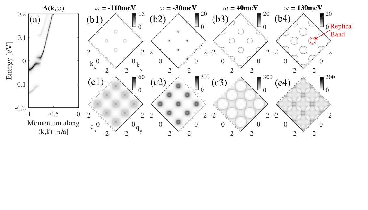
Our QPI results are summarized in Figs. 12 and 13. The spectral function for our “bare” electronic structure, including the effects of the $e$-$ph$ interaction, is shown in Fig. 12(a) for reference. The relevant model parameters are given in the figure caption. Constant energy cuts of the spectral function are shown Figs. 12(b1)–(b4) for energies located inside the occupied replica band [$-110$ meV, panel (b1)], inside the occupied states of the main band [$-30$ meV, panel (b2)], inside the unoccupied states of the main band [$40$ meV, panel (b3)], and inside the unoccupied replica band [$130$ meV, panel (b4)]. In Fig. 12(b1)–(b3) one can see a clear ring-like feature corresponding to the single replica or main band that is intersected at these energies; however, in Fig. 12(b4), a double ring structure is observed where the inner ring corresponds to the replica band and the outer ring corresponds to the main band.

This electronic structure is reflected in the corresponding QPI spectra, shown in Fig. 12(c1)–(c4), respectively. The maps in Figs. 12(c1)–(c3) have a clear ring-like structure with a radius ${\bf q}=2{\bf k}(\omega)$, where ${\bf k}(\omega)$ is a vector spanning the constant energy contours. These features resemble what one would expect for a simple single band system [64, 65]. At $\omega=130$ meV, however, the QPI pattern develops a double ring structure, as one would might expect from the topology of the main and replica bands shown in Fig. 12(b4). Based on the geometry of the features we can assign the outer QPI peak to intraband scattering within the main band and inner QPI peak to interband scattering between the unoccupied states of the replica and main bands. We also see a very weak feature due to intraband scattering within the replica band, however, it is very difficult to resolve in this image. The intensity of these features also follows the hierarchy of spectral weight associated with the type of band. The relative intensity of these features are also shown in Fig. 13.

These results establish that the replica bands can be observed in the QPI spectra and therefore FT-STS could in principle study these features, particularly on the unoccupied side of $E_{\mathrm{F}}$. In this case, the QPI peaks due to the replica bands will appear similar to regular bands at a given bias voltage albeit with a reduced intensity; however, the dispersion and spectral weight of these features will be quite different. To illustrate this, we plot the QPI intensity along the ${\bf q}=(q,q)$ line as a function of energy in order to track the dispersion of the QPI peaks. Fig. 13(a1) presents this information as a false colour image while Fig. 13(a2) presents it as a contour plot in order to highlight the features with weaker intensity. If a QPI peak is due to intraband scattering in the main band, then it will disperse towards ${\bf q}=0$ as the bias voltage is tuned towards the top or bottom of the band [64]. This can be clearly seen in Fig. 13(a1) from the most intense feature. In contrast, the dispersion of a peak due to inter or intraband scattering to a replica band will be different due to the extinction of the replica band’s spectral weight at ${\bf k}_{\mathrm{F}}$. This is apparent in Fig. 13(a1) and Fig. 13(a2), where the intensities of the interband scattering feature at positive energies and the intraband scattering feature at negative energies sudden disappears at the energy where the replica band disappears. This is another unique spectral fingerprint of a replica band.

While there have been several QPI studies conducted on the FeSe/STO system [20, 19], to the best of our knowledge no indications of the replica bands have been observed. One study by Huang et al. (Ref. [19]) found evidence for an electron-like and located 75 meV above $E_{\mathrm{F}}$; however, the measurements of the tunneling decay length indicated that this band was centered at the $\Gamma$-point rather than the $M$-point. This rules out the possibility that this feature is due to the replica expected for the electron pockets at the $M$-point. However, we also note that nearly all of the QPI studies completed to date have focused on energy windows of less than 80 meV of the Fermi level [20, 19]. This is outside the region where the replica band are expected, based on the phonon energy scale inferred by ARPES [11]. It would therefore be interesting to extend these studies to higher bias voltages in order to determine if the features shown in Fig. 13 can be observed. This will be a challenging task, however, as our calculations have shown that the replica QPI peaks are much weaker in intensity than the main QPI peaks.

References

- [1] F.- C. Hsu et al., Proceedings of the National Academy of Sciences 105, 14262 (2008).
- [2] Q. L. Wang et al., Chin. Phys. Lett. 29, 037402 (2012).
- [3] D. F. Liu et al., Nature Commun. 3, 931 (2012).
- [4] K. Liu, Z.-Y. Lu, and T. Xiang, Phys. Rev. B 85, 235123 (2012).
- [5] F. Zheng, Z. Wang, W. Kang, and P. Zhang, Scientific Reports 3, 2213 (2013).
- [6] S. L. He et al., Nature Mater. 12, 605 (2013).
- [7] S. Tan et al., Nature Mater. 12, 634640 (2013).
- [8] W. H. Zhang et al., Phys. Rev. B 89, 060506(R) (2014).
- [9] R. Peng et al., Nature Commun. 5, 5044 (2014).
- [10] R. Peng et al., Phys. Rev. Lett. 112, 107001 (2014).
- [11] J. J. Lee et al., Nature 515, 245 (2014).
- [12] B. Li, Z. W. Xing, G. Q. Huang, and D. Y. Xing, Journal of Applied Physics 115, 193907 (2014).
- [13] X. Liu et al., Nature Commun. 5, 5047 (2014).
- [14] D.-H. Lee, Chinese Physics B 11, 117405 (2015).
- [15] L. Rademaker, Y. Wang, T. Berlijn, and S. Johnston, arXiv:1507.03967 (2015).
- [16] J.F. Ge et al., Nature Mater. 14, 285 (2015).
- [17] Y. Miyata, K. Nakayama, K. Sugawara, T. Sato, and T. Takahashi, Nat. Mater. 14 775 (2015).
- [18] S. Coh, M. L. Cohen, S. G. Louie, New J. Phys. 17, 073027 (2015).
- [19] D. Huang et al., Phys. Rev. Lett. 115, 017002 (2015).
- [20] Q. Fan et al., Nature Phys. 11, 946 (2015).
- [21] C.-L. Song, et al., arXiv:1511.02007 (2015).
- [22] J. J. Seo, et al., arXiv:1511.07950 (2015).
- [23] J. Shiogai, Y. Ito, T. Mitsuhashi, T. Nojima, and A. Tsukazaki, arXiv:1510.00175 (2015).
- [24] P. Zhang et al., arXiv:1512.01949 (2015).
- [25] G. Zhou et al., arXiv:1512.01948 (2015).
- [26] Y. Zhang, J. J. Lee, R. G. Moore, W. Li, M. Yi, M. Hashimoto, D. H. Lu, T. P. Devereaux, D.-H. Lee, and Z.-X. Shen, Superconducting gap anisotropy in monolayer FeSe thin film. arXiv:1512.06322 (2015).
- [27] Z.-X. Li, F. Wang, H. Yao, D.-H. Lee, arXiv:1512.06179 (2015).
- [28] E. Dagotto, Rev. Mod. Phys. 85, 849 (2013).
- [29] J. G. Guo et al., Phys. Rev. B 82, 180520 (2010).
- [30] L. Zhao et al., arXiv:1505.06361 (2015).
- [31] I. Mazin, D.J. Singh, M.D. Johannes, and M.-H. Du, Phys. Rev. Lett. 101, 057003 (2008).
- [32] P. J. Hirschfeld, M. M. Korshunov, I. I. Mazin, Rep. Prog. Phys. 74, 124508 (2011).
- [33] M. Burrard-Lucas et al., Nature Mater. 12, 15 (2013).
- [34] G. Varelogiannis, A. Perali, E. Cappelluti, and L. Pietronero, Phys. Rev. B 54, R6877 (1996).
- [35] M. L. Kulić and O. V. Dolgov, Phys. Stat. Sol. (b) 242, 151 (2005) and references therein.
- [36] M. L. Kulić and R. Zeyher, Phys. Rev. B 49, 4395(R) (1994).
- [37] A. Aperis, P. Kotetes, G. Varelogiannis, and P. M. Oppeneer, Phys. Rev. B 83, 092505 (2011).
- [38] N. Bulut and D. J. Scalapino, Phys. Rev. B 54, 14971 (1996).
- [39] X. Chen, A. Linscheid, S. Maiti, and P. J. Hirschfeld, Phys. Rev. B 92, 224514 (2015);
- [40] L. P. Gor’kov, arXiv:1510.03327 (2015).
- [41] N. Choudhury, E. J. Walter, A. I Kolesnikov, and C.-K. Loong, Phys. Rev. B 77, 134111 (2008).
- [42] B. Li, Z. W. Xing, G. Q. Huang, and D. Y. Xing, Journal of Applied Physics 115, 193907 (2014).
- [43] Y. Wang, A. Linscheid, T. Berlijn, and S. Johnston (to be published).
- [44] F. Marsiglio, M. Schossmann, and J. P. Carbotte, Phys. Rev. B 37, 4965 (1988).
- [45] G. D. Mahan, Many-Particle Physics. 3rd Ed. (2000).
- [46] A. B. Migdal, Sov. Phys. JETP 34, 996 (1958).
- [47] L. Zhu, P. J. Hirschfeld, and D. J. Scalapino, Phys. Rev. B 70, 214503 (2004).
- [48] S. H. Hong et al., Phys. Rev. Lett. 113, 057001 (2014).
- [49] C. Grimaldi, L. Pietronero, and S. Strässler, Phys. Rev. B 52, 10530 (1995).
- [50] L. Pietronero, S. Strässler, and C. Grimaldi, Phys. Rev. B 52, 10516 (1995).
- [51] For recent reviews, see T. Cuk et al., Phys. Stat. Sol. (b) 242, 11 (2005); J.P. Carbotte, T. Timusk, and J. Hwang, Rep. Prog. Phys. 74, 066501 (2011).
- [52] O. V. Danylenko, O. V. Dolgov, M. L. Kulić, and V. Oudovenko, Eur. Phys. J. B 9, 201 (1999).
- [53] S. Johnston and T. P. Devereaux, Phys. Rev. B 81, 214512 (2010).
- [54] G. Santi, T. Jarlborg, M. Peter, and M. Weger, Physica C 259, 253 (1996).
- [55] W. McMillan and J. Rowell, in Superconductivity, edited by R. D. Parks (Dekker, New York, 1969) Vol. 1.
- [56] G. L. de Castro, C. Berthod, A. Piriou, E. Giannini, and Ø. Fischer, Phys. Rev. Lett. 101, 267004 (2008).
- [57] J. E. Hoffman, et al., Science 297, 1148 (2002).
- [58] T.-M. Chuang et al., Science 327, 181 (2010)
- [59] S. Chi et al., Phys. Rev. Lett. 109, 078002 (2012).
- [60] M. P. Allan, et al., Science 336, 563 (2012).
- [61] T. Hänke et al., Phys. Rev. Lett. 108, 127001 (2012).
- [62] P. J. Hirschfeld, D. Altenfeld, I. Eremin, I. I. Mazin, Phys. Rev. B 92, 184513 (2015).
- [63] Q.-H. Wang and D.-H. Lee, Phys. Rev. B 67, 020511 (2003).
- [64] S. Grothe, S. Johnston, S. Chi, P. Dosanjh, S. A. Burke, and Y. Pennec, Phys. Rev. Lett. 111, 246804 (2013).
- [65] L. Capriotti, D. J. Scalapino, and R. D. Sedgewick, Phys. Rev. B 68, 014508 (2003).
- [66] Y. Bang, New J. Phys. 16, 023029 (2014);
- [67] F. Wang, F. Yang, M. Gao, Z.-Y. Lu, T. Xiang, and D.-H. Lee, Europhys. Lett. 93, 57003 (2011);
- [68] T. S. Nunner, J. Schmalian, and K. H. Bennemann, Phys. Rev. B 59, 8859 (1999).
- [69] Y. Bang, Phys. Rev. B 78, 075116 (2008).