The K2-ESPRINT Project IV: A Hot Jupiter in a Prograde Orbit with a Possible Stellar Companion
Abstract
We report on the detection and early characterization of a hot Jupiter in a 3-day orbit around K2-34 (EPIC 212110888), a metal-rich F-type star located in the K2 Cycle 5 field. Our follow-up campaign involves precise radial velocity (RV) measurements and high-contrast imaging using multiple facilities. The absence of a bright nearby source in our high-contrast data suggests that the transit-like signals are not due to light variations from such a companion star. Our intensive RV measurements show that K2-34b has a mass of , confirming its status as a planet. We also detect the Rossiter-McLaughlin effect for K2-34b and show that the system has a good spin-orbit alignment ( degrees). High-contrast images obtained by the HiCIAO camera on the Subaru 8.2-m telescope reveal a faint companion candidate ( mag) at a separation of . Follow-up observations are needed to confirm that the companion candidate is physically associated with K2-34. K2-34b appears to be an example of a typical “hot Jupiter,” albeit one which can be precisely characterized using a combination of K2 photometry and ground-based follow-up.
Subject headings
planets and satellites: detection – stars: individual (EPIC 212110888, K2-34) – techniques: photometric – techniques: radial velocities – techniques: spectroscopicI. Introduction
Hot Jupiters have been subjected to intensive studies of their orbits and atmospheres. When one imagines a “typical” hot Jupiter, one would think of a jovian planet orbiting a relatively metal-rich solar-type star within 3 days. Many other characteristics of hot Jupiters have been discussed in the literature, including the inflation of their radii when the insolation from the central stars becomes strong [11, e.g.,]. Hot Jupiters, at least around relatively cool stars ( K), generally have circular orbits aligned with their host stars’ spin axes [51, 2]. Moreover, hot Jupiters are generally isolated up to a certain distance from their host stars [42] with the exception of WASP-47 [3], but are likely to have some “friend(s)” at longer orbital separations. These friends are outer planetary and/or stellar companions, and have been revealed by long-term RV monitoring and high-contrast imaging campaigns [20, 27, 26, e.g.,]. However, such intensive studies have not settled the serious issues for both the origin of hot Jupiters and their properties, and we have not reached a consensus for the formation and evolution of hot Jupiters.
The Kepler satellite’s second mission, K2, has provided new opportunities to search and characterize transiting planets including hot Jupiters. K2 has already discovered many outstanding systems including possibly rocky planets around cool dwarfs [8, 33] and a disintegrating minor planet around a white dwarf [50]. To find and characterize the unique planetary systems detected by K2, we initiated the new collaboration ESPRINT, Equipo de Seguimiento de Planetas Rocosos Intepretando sus Transitos, which has already confirmed/validated a disintegrating rocky planet [35, ESPRINT I:], small planets around solar-type stars [49, ESPRINT II:] and a super-Earth/mini-Neptune around a mid-M dwarf, for which intensive follow-up studies are expected [18, ESPRINT III:].
In this paper, we report the discovery and early characterization of a hot Jupiter, detected by our pipeline applied to the K2 Cycle 5 field stars. Our target, K2-34, is an F-type star with an effective temperature of K, as inferred from its colors. The top part of Table 1 summarizes the properties of K2-34 as collected from the SDSS and 2MASS catalogs [1, 40]. Our earlier analysis implied that the planetary candidate, K2-34b, orbits its central star with a period extremely close to 3 days. With intensive follow-up observations including radial velocity (RV) measurements and high-contrast imaging, we confirm that K2-34b is indeed a hot Jupiter orbiting K2-34. Our analysis suggests the hot Jupiter to be a typical, but still important, example of its class, exhibiting many of the properties described above.
The rest of the paper is organized as follows. We describe our pipeline to reduce the K2 data and detect planetary candidates in K2 field 5 (Section II.1); Section II.2 describes our follow-up campaign with RV measurements by the High Accuracy Radial velocity Planet Searcher North (HARPS-N) on the 3.6-m Telescopio Nazionale Galileo (TNG) and High Dispersion Spectrograph (HDS) on the Subaru 8.2-m telescope, in which a complete spectroscopic transit of K2-34b is covered. Section II.3 presents lucky imaging at 1.52-m Telescopio Carlos Sánchez (TCS) and adaptive-optics (AO) imaging with Subaru/HiCIAO. We perform a simultaneous fit to the reduced K2 light curve and observed RVs by the two spectrographs, including the modeling of the Rossiter-McLaughlin (RM) effect [29, 52, e.g.,] of K2-34b in Section III. Section IV is devoted to discussion and summary.
II. Observations and Data Reductions
II.1. K2 Photometry
K2-34 was observed from the of April to the of July 2015 as a pre-selected target star of K2 Campaign 5. We downloaded the images of K2-34 from the MAST website. The production of detrended K2 light curves by our collaboration was described in detail in the ESPRINT I paper [35]. We then searched the light curves for transiting planet candidates with a Box-Least-Squares routine [21, 19] using the optimal frequency sampling described by Ofir [28]. K2-34 was clearly detected with a signal-to-noise ratio (SNR) of 15.5. A linear ephemeris analysis of the individual transits yielded a best-fit period of days and a mid-transit time of (BJD). Figure 1 plots the full reduced light curve; the deep transits (marked by red lines) are clearly visible.

| Parameter | Value |
|---|---|
| (Stellar Parameters from the SDSS and 2MASS Catalogs) | |
| RA | |
| Dec | |
| (mag) | |
| (mag) | |
| (mag) | |
| (mag) | |
| (mag) | |
| (mag) | |
| (mag) | |
| (Spectroscopic Parameters) | |
| (K) | |
| (dex) | |
| (dex) | |
| (km s-1) | |
| (km s-1) | |
| (km s-1; assumed) | |
| (Derived Parameters by Empirical Relation) | |
| () | |
| () | |
| () | |
| (Derived Parameters by Y2 Isochrone) | |
| () | |
| () | |
| () | |
| age (Gyr) | |
II.2. High Dispersion Spectroscopy
II.2.1 TNG/HARPS-N
In order to confirm the planetary nature of K2-34b detected above, we observed K2-34 with TNG/HARPS-N for precise RV measurements on 2015 November 18-25 UT as part of the observing program CAT15B_79. HARPS-N [7] is a fiber-fed, echelle, thermally stable spectrograph in a vacuum, located on TNG at the Roque de los Muchachos Observatory (ORM) on La Palma, Spain. It covers the visible wavelength range between 383 nm and 693 nm with a resolving power of . TNG/HARPS-N RV measurements and their uncertainties were obtained with the G2 cross-correlation mask using the DRS pipeline, which is based on the weighted CCF method [32]. Thirteen RV measurements collected during the TNG/HARPS-N run allowed us to confirm the planetary nature of K2-34b, and to designate the target for a spectroscopic transit observation from Mauna Kea on November 27 in order to measure the RM effect of the system. Our TNG/HARPS-N measurements are presented in Table 2.
| BJD | value (m s-1) | error (m s-1) |
|---|---|---|
II.2.2 Subaru/HDS
We also observed K2-34 with Subaru/HDS for precise RV measurements on 2015 November 26-28 UT and 2016 February 2 UT. We employed the standard I2a setup with Image Slicer #2, covering the spectral region between nm with [44]. For the precise RV measurements, we used the iodine (I2) cell and have the stellar light transmit through that cell to imprint the rich absorption lines of I2 in the stellar spectra. On November 27, a spectroscopic transit was visible from Mauna Kea, and we took that opportunity to measure the RM effect of the system, covering the whole transit of K2-34b (2 hours). On the same night, we obtained the stellar spectrum without the I2 cell for a template in the RV analysis as well as for the detailed spectroscopic characterization of K2-34. During the twilight, we also obtained a flat-lamp spectrum transmitted through the I2 cell so that we can estimate the instrumental profile (IP) of HDS on that observing night. During the November run, we had some clouds throughout the week on Mauna Kea, and the typical photon counts of the raw spectra were about half of what we had initially expected.
We reduced the raw data in a standard manner using the IRAF package to extract the wavelength-calibrated, one-dimensional (1D) spectra. The signal-to-noise ratio (SNR) of the 1D spectra was typically 60 per pixel. We then input the Iin spectra into the RV pipeline to extract the relative RV values with respect to the Iout template spectrum. The RV analysis for Subaru/HDS is described in detail in Sato et al. [36], Sato et al. [37]. The resulting RV values are listed in Table 3 along with their uncertainties.
| BJD | value (m s-1) | error (m s-1) |
|---|---|---|
We measured the equivalent widths for Fe I and Fe II lines of the Iout template spectrum, making it possible to estimate the atmospheric parameters of K2-34. As described in Takeda et al. [45], Takeda et al. [46], we estimated the stellar effective temperature , surface gravity , metallicity [Fe/H], and microturbulent velocity from the excitation and ionization equilibria. We also measured the projected rotational velocity of the star by convolving a theoretically synthesized spectrum with the rotation plus macroturbulence broadening kernel [12, the radial-tangential model:] and the IP of HDS. Following Hirano et al. [15], Hirano et al. [16], we adopted the empirical relation by Valenti & Fischer [48] for the macroturbulent velocity as
| (1) |
The results of these measurements are summarized in the second part of Table 1.
To estimate the physical parameters of the star, we converted the atmospheric parameters into mass and radius (and density), employing two different methods. We first used the empirical relations for stellar mass and radius derived by Torres et al. [47], which is based on physical parameters measured using detached binaries. We also converted the atmospheric parameters using the Yonsei-Yale (Y2) isochrone model [54]. For both cases, we ran Monte Carlo simulations to estimate the uncertainties for the physical parameters by randomly generating the sets of atmospheric parameters assuming Gaussian errors. Since the uncertainties for atmospheric parameters listed in Table 1 are all statistical errors, we quadratically added a systematic error of K for the effective temperature to account for the systematics estimated by Bruntt et al. [5], who compared the luminosity-based effective temperatures with the spectroscopically measured values as presented here. The resulting parameters, including their uncertainties, are summarized in the bottom parts of Table 1. The mass and radius estimated by the two techniques are consistent with each other within . Since the uncertainties for the empirical mass and radius take into account the systematic errors in the empirical relation, we use those estimates for the rest of this paper.
II.3. High Contrast Imaging
We obtained high-contrast images of K2-34 to search for stellar companions, and to exclude the possibility that the transit signal is a false positive from a background eclipsing binary. Our data, described below, consist of lucky imaging observations with the FastCam camera and adaptive optics imaging with HiCIAO on the Subaru Telescope.
II.3.1 TCS/FastCam Lucky Imaging Observations
On 2015 November 15 UT, 20,000 individual frames of K2-34 were collected in the band using FastCam [31] at TCS in the Observatorio del Teide, Tenerife, with 50 ms exposure time for each frame. FastCam is an optical imager with a low noise EMCCD camera which allows to obtain speckle-featuring non-saturated images at a fast frame rate [22, see].
In order to construct a high resolution, diffraction limited, long-exposure image, the individual frames were bias subtracted, aligned and co-added using a Lucky Imaging (LI) algorithm [23, see]. The LI selection is based on the brightest speckle in each frame, which has the highest concentration of energy and represents a diffraction limited image of the source. Those frames with a larger count number at the brightest speckle are the best ones. The percentage of the best frames chosen depends on the natural seeing conditions and the telescope diameter and is based on a trade between a sufficiently high integration time, given by a higher percentage, and a good angular resolution, obtained by co-adding a lower amount of frames. Figure 2 presents the high resolution image constructed by co-addition of the 30% of the best frames, i.e. with 300-second total exposure time. The combined image achieved at , and no bright companion was detectable in the images within .

II.3.2 Subaru/HiCIAO Observations
We used adaptive optics imaging on the Subaru Telescope to rule out the presence of a background eclipsing binary at smaller angular separations and to search for faint stellar companions. Our observations were conducted on 2015 December 30 UT using the adaptive optics system AO188 [13] and the high-contrast near-infrared camera HiCIAO [43]. Using K2-34 as a natural-guide star, we acquired 60 dithered frames with individual integration times of 15 s for a total integration time of 900 s. The point spread functions (PSFs) of the primary star in these images were intentionally saturated within typically , to search for faint companions. We also took unsaturated images with a 9.74% neutral-density filter to verify the star’s position and flux. We obtained images of the globular cluster M5 for astrometric calibration.
II.3.3 HiCIAO Data Reductions
We reduced our HiCIAO data using the ACORNS pipeline, described in [4]. We removed correlated read noise, masked hot pixels, flat-fielded, and corrected instrumental distortion by comparing images of the globular cluster M5 with archival data from the Hubble Space Telescope. We then aligned the images, but did not apply high-contrast algorithms to suppress diffracted starlight.
We combined all the saturated images to find a faint companion candidate (CC) around K2-34 (see Figure 3). However, the CC appears to be embedded in the bright halo of primary star’s PSF. To suppress the halo, we applied high-pass filter to each saturated image after the image registration. We used a median filter with a width of 4 PSF full widths at half maximum (FWHM; 1 FWHM 54 mas), subtracting the filtered image from each of our original frames. The lower panel of Figure 3 displays the final combined image, on which the CC is clearly detected. We measure a centroid of CC and estimate the separation and position angles between the CC and primary star to be 361.3 3.5 mas and 20677 062, respectively. The CC’s position was measured in the frames where the primary star’s PSF is saturated. We corrected the primary star’s centroids using the unsaturated frames whose acquisitions were interspersed through the data-acquisition sequence for the saturated frames.
We performed aperture photometry for the CC on the combined, high-pass-filtered image shown in the bottom panel of Figure 3. It is notable that the high-pass filter decreases the flux of CC. We estimated and recovered the flux loss (35%) based on the reductions for the images with injected artificial sources. We measure a final, corrected -band contrast of mag. This brightness contrast was derived using the primary star’s flux in the unsaturated frames, for which a simultaneous photometry of the primary star and CC is prohibited. Then, the variation of AO correction is attributed to the photometry uncertainty, and we consider that the error term related to this variation is represented by the scatter of the photometry of unsaturated PSFs.

III. Global Analysis
The high-contrast images by TCS/FastCam (in band) and Subaru/HiCIAO (in band) show no nearby source bright enough to cause a transit-like signal as deep as . A background eclipsing binary, even if it achieved the maximum possible occulation (50%), would need to be no more than 70 times (4.6 magnitudes) fainter than K2-34. Our observations, combined with SDSS archival images, confirm that no such sources exist between and 20′′. It is still possible that a relatively bright binary companion is present within from K2-34, but visual inspection of the HDS spectrum did not show any secondary peak as shown in Figure 4. Along with the fact that the observed RVs clearly show the presence of a planet-sized companion, whose RV variation is synchronous with the predicted phase from the K2 transits, we conclude that the periodic dimming seen in the K2 light curve is associated with a jovian planet orbiting K2-34.

Here, we attempt to simultaneously fit the K2 light curve with the RVs observed by HARPS-N and HDS. The fitting procedure is similar in many aspects to those described in Hirano et al. [14] and Sato et al. [38]. We use the following statistics in the global fit:
| (2) | |||||
where , , and are th observed K2 flux, HDS RV value, and HARPS RV value, and , , and are their errors, respectively. To compute the model flux observed by K2, we integrate the transit model by Ohta et al. [30] over the cadence of the K2 observation (29.4 minutes).
For the RV model, we adopt the following equations:
| (3) | |||||
| (4) |
where , , , and , , are the RV semi-amplitude, true anomaly, orbital eccentricity, argument of periastron, and RV offsets for the HDS and HARPS data sets, respectively. Since the HDS data set covered a complete transit of K2-34b, we introduce the velocity anomaly term due to the RM effect for that data set only. We adopt the analytic formula by Hirano et al. [17], in which is computed in terms of the projected rotational velocity . For other spectroscopic parameters that appear in Equation (16) of Hirano et al. [17], we assume the Gaussian and Lorentzian widths of km s-1 and km s-1, and the macroturbulent velocity of km s-1 as in Section II.2.2. We here neglect the convective blue-shift [39], since its impact is small enough ( m s-1 at the most) compared with the internal errors of Subaru/HDS RV data (10 m s-1).
Assuming that the likelihood is proportional to , we run a Markov Chain Monte Carlo (MCMC) simulation to estimate the global posterior distribution of the fitting parameters. The fitting parameters in our model are orbital period , time of the transit center , scaled semi-major axis , transit impact parameter , planet-to-star radius ratio , and limb-darkening parameters and for the K2 data set assuming a quadratic law, , , , , the projected obliquity , , and . Among these, , , , , , , , are related to both the light curve and RV data sets, but the others are for RV data only (except the limb-darkening coefficients). Since limb-darkening coefficients are weakly constrained from the K2 transit curve, we put weak Gaussian priors on and , with their centers being 0.65 and 0.08, respectively, and dispersions of , based on the theoretical values by Claret & Bloemen [6] for the Kepler band. The RM velocity anomaly also weakly depends on the limb-darkening coefficients. The RV precision and sparse time sampling of the Subaru/HDS dataset, however, make the fit of those coefficients almost impossible, and we opted to fix them at and based on the theoretical values for the band [6]. We note that we allow the orbital period to vary rather than fix it at the value from the light curve analysis alone. In this way, the ephemeris of K2-34b is globally determined from the light curve and RV data, and the uncertainty in modeling the RM effect reflects the uncertainty of the period.
We use our customized code [14, e.g.,] to perform the global fit, in which Equation (2) is first minimized by the Nelder-Mead simplex method [34, e.g.,] and then the step size for each parameter is iteratively optimized, before running MCMC steps to estimate the global posterior. Since the accurate uncertainty for each flux value in K2 data is difficult to infer, we scaled so that the reduced for the K2 data set becomes approximately unity. We take the median, 15.87 and 84.13 percentiles of the maginalized posterior for each fitting parameter to provide the best-fit value and its uncertainties, which are listed in Table 4. The observed data along with the best-fit models are displayed in Figures 5, 6, and 7, for the phase-folded K2 light curve, orbital RVs, and RM velocity anomaly, respectively.


The best-fit model indicates that K2-34b is a typical hot Jupiter in a 3-day, prograde orbit ( degrees). Based on the best-fit model parameters in the global fit as well as K2-34’s physical parameters, we also compute K2-34b’s physical and orbital parameters, including the planet mass , radius , density , orbital inclination , and semi-major axis . The result is also summarized in Table 4; the planet is consistent with a slightly inflated jovian planet, in a circular orbit (within ). The stellar density from the transit curve alone is estimated to be , which agrees with the spectroscopically measured stellar density (Table 1) with , reinforcing the idea that K2-34b is indeed transiting the F star.
The residual of the RM velocity anomaly in Figure 7 seems to exhibit a possible time-correlated noise, where each RV residual could be correlated with the adjacent ones. To test if this is the case or not, we computed Pearson’s correlation coefficient between the adjacent RV residual values in Figure 7. We then ran a Monte Carlo simulation of steps to estimate its value, where we permutated the RV residuals randomly and recorded each correlation coefficient between the adjacent RV residuals for each dataset (step). Consequently, we obtained and found that its value is high enough (), implying that the observed RV residuals have no significant correlation with the next ones (i.e., time-correlated noise was not observed).
We note that is a projected obliquity and the true, 3-dimensional (3D) spin-orbit angle is not known; does not necessarily mean that the orbit is aligned. One way to break this degeneracy is to measure the stellar inclination , which is defined as the angle between the line-of-sight and stellar spin axis by the combination of the stellar rotation period, radius, and projected rotation velocity [15, e.g.,]. We inspected the periodogram of K2-34’s light curve and found that there was a peak around days, which could be ascribed to the rotation period of K2-34, which is also expected by scaling the Sun’s rotation period ( days) by . If this peak indeed corresponds to the period of rotation, the rotation velocity at the stellar equation is estimated as km s-1 based on the listed in Table 1. Comparing this value with the observed , we expect that is close to , suggesting a small 3D spin-orbit angle.
| Parameter | Value |
|---|---|
| (Fitting Parameters) | |
| (days) | |
| (BJD) | |
| (m s-1) | |
| (km s-1) | |
| (∘) | |
| (m s-1) | |
| (m s-1) | |
| (Derived Parameters) | |
| () | |
| () | |
| () | |
| (∘) | |
| (AU) | |
IV. Discussion and Summary
We have conducted intensive follow-up observations for a hot Jupiter candidate, K2-34b, which was detected by our pipeline in an analysis of K2 field 5 stars. Our RV follow-up, along with the absence of a bright nearby source () in the high-contrast images, confirm the planetary nature of K2-34; we have determined the mass and radius of the planet to be and , respectively. Its central star, K2-34, is a relatively metal-rich, F-type star, which is typical of hot-Jupiter hosts.
We detected the velocity anomaly during the transit observed by HDS on November 27, with significance. Modeling of the RM effect implies that the orbit of K2-34b is prograde with respect to the stellar spin; we estimate the best-fit value for the projected obliquity as degrees. To verify our result, we also tested the global fit with a Gaussian prior distribution for based on the spectroscopically measured value, and obtained a fully consistent result ( degrees). This small obliquity is consistent with the well-known finding that stars cooler than K generally have a small obliquity, while hotter ones tend to be misaligned [51, e.g.,]. K2-34’s effective temperature is K, which is close to the alignment/misalignment divide, making it an important sample for future statistical analyses on observed obliquities.
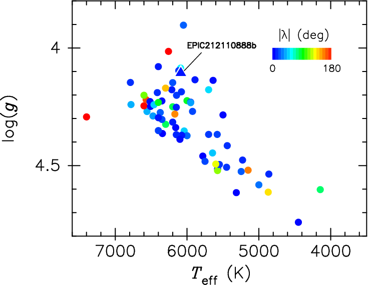
K2-34 is located around an edge of the main sequence in the plane (Figure 8). This region of stellar evolution has fewer measurements of the stellar obliquity. One possible channel for the formation of hot Jupiters is dynamical processes (e.g., planet-planet scatterings) followed by tidal interactions between planets and their hosts [25, 10, e.g.,]. Tidal interactions also tend to damp the stellar obliquity, but the precise timescale of this obliquity damping is not known and believed to depend on the stellar type [51, 53]. In this context, a comparison between the timescales for the obliquity damping by tides and actual system ages could become an important clue. Considering that ages are generally better constrained for the slightly evolved, but still hot stars such as K2-34 than for their cooler counterparts, more obliquity measurements for those stars will provide additional insight into the tidal evolution of hot Jupiters.
It would be also of interest to discuss the observed obliquity in terms of host star’s mass. Spalding & Batygin [41] described that an alternative explanation for the observed trend of stellar obliquity is that magnetic star-disk torques act to damp non-zero stellar obliquities of less massive stars. Since the magnetic field of massive stars () is much weaker by an order of magnitude, the stellar obliquity, which could be primordially enhanced by e.g., an outer companion, is preserved and a spin-orbit misalignment is likely observed around those stars [41, see Figure 1 in]. Provided that K2-34’s mass is , the low obliquity in this system could be a new exception to the observed dependence of stellar obliquity on the stellar mass.
AO imaging using Subaru/HiCIAO has revealed a possible companion with at a separation of . If this faint source is indeed bound to K2-34, the projected distance between the two components is estimated as AU assuming a distance to K2-34 of pc based on its apparent and estimated absolute magnitudes. One can also estimate the absolute magnitude of the hypothetical stellar companion as mag using an isochrone [9, e.g.,], which corresponds to a mid-M dwarf whose mass is . The absolute Kepler magnitude of this CC is also estimated as mag. Considering K2-34’s absolute magnitude of , we can safely neglect the impact of dilution in the K2 transit curve (). If this CC is indeed bound to K2-34, it also satisfies a general trend that hot Jupiters have outer giant planets and/or stellar companions [20, 27, 26, e.g.,], but future follow-up observations are required to prove the physical association by checking the common proper motion and/or detecting the CC in a different observing band.
The relative brightness of the host star (e.g., mag) makes K2-34b a good target for further follow-up to characterize its atmosphere. With the period so close to 3 days ( days), however, transit follow-ups from the ground are only possible around a certain longitude on the Earth for long intervals. This in turn means that its transits are visible every 3 days at certain observatories, and unusually accurate characterization may be possible through repeated observations of transits.
Note: After completing the work described herein, we became aware of the independent discovery and characterization of K2-34b by Lillo-Box et al. [24]. Our measurements of the stellar and planetary properties are in agreement with theirs.
Facilities: Subaru (HDS, HiCIAO), TNG (HARPS-N), TCS (FastCam)
References
- [1] Ahn, C. P., Alexandroff, R., Allende Prieto, C., et al. 2012, ApJS, 203, 21
- [2] Albrecht, S., Winn, J. N., Johnson, J. A., et al. 2012, ApJ, 757, 18
- [3] Becker, J. C., Vanderburg, A., Adams, F. C., Rappaport, S. A., & Schwengeler, H. M. 2015, ApJ, 812, L18
- [4] Brandt, T. D., McElwain, M. W., Turner, E. L., et al. 2013, ApJ, 764, 183
- [5] Bruntt, H., Bedding, T. R., Quirion, P.-O., et al. 2010, MNRAS, 405, 1907
- [6] Claret, A., & Bloemen, S. 2011, A&A, 529, A75
- [7] Cosentino, R., Lovis, C., Pepe, F., et al. 2012, in Proc. SPIE, Vol. 8446, Ground-based and Airborne Instrumentation for Astronomy IV, 84461V
- [8] Crossfield, I. J. M., Petigura, E., Schlieder, J. E., et al. 2015, ApJ, 804, 10
- [9] Dotter, A., Chaboyer, B., Jevremović, D., et al. 2008, ApJS, 178, 89
- [10] Fabrycky, D., & Tremaine, S. 2007, ApJ, 669, 1298
- [11] Fortney, J. J., Baraffe, I., & Militzer, B. 2010, Giant Planet Interior Structure and Thermal Evolution, ed. S. Seager, 397–418
- [12] Gray, D. F. 2005, The Observation and Analysis of Stellar Photospheres, ed. Gray, D. F.
- [13] Hayano, Y., Takami, H., Oya, S., et al. 2010, in Proc. SPIE, Vol. 7736, Adaptive Optics Systems II, 77360N
- [14] Hirano, T., Masuda, K., Sato, B., et al. 2015, ApJ, 799, 9
- [15] Hirano, T., Sanchis-Ojeda, R., Takeda, Y., et al. 2012, ApJ, 756, 66
- [16] —. 2014, ApJ, 783, 9
- [17] Hirano, T., Suto, Y., Winn, J. N., et al. 2011, ApJ, 742, 69
- [18] Hirano, T., Fukui, A., Mann, A. W., et al. 2016, ApJ, 820, 41
- [19] Jenkins, J. M., Caldwell, D. A., Chandrasekaran, H., et al. 2010, ApJ, 713, L87
- [20] Knutson, H. A., Fulton, B. J., Montet, B. T., et al. 2014, ApJ, 785, 126
- [21] Kovács, G., Zucker, S., & Mazeh, T. 2002, A&A, 391, 369
- [22] Labadie, L., Rebolo, R., Villó, I., et al. 2011, A&A, 526, A144
- [23] Law, N. M., Mackay, C. D., & Baldwin, J. E. 2006, A&A, 446, 739
- [24] Lillo-Box, J., Demangeon, O., Santerne, A., et al. 2016, ArXiv e-prints, arXiv:1601.07635
- [25] Nagasawa, M., & Ida, S. 2011, ApJ, 742, 72
- [26] Neveu Van Malle, M., Queloz, D., Triaud, A. H. M. J., et al. 2015, in AAS/Division for Extreme Solar Systems Abstracts, Vol. 3, AAS/Division for Extreme Solar Systems Abstracts, 101.06
- [27] Ngo, H., Knutson, H. A., Hinkley, S., et al. 2015, ApJ, 800, 138
- [28] Ofir, A. 2014, A&A, 561, A138
- [29] Ohta, Y., Taruya, A., & Suto, Y. 2005, ApJ, 622, 1118
- [30] —. 2009, ApJ, 690, 1
- [31] Oscoz, A., Rebolo, R., López, R., et al. 2008, in Proc. SPIE, Vol. 7014, Ground-based and Airborne Instrumentation for Astronomy II, 701447
- [32] Pepe, F., Mayor, M., Galland, F., et al. 2002, A&A, 388, 632
- [33] Petigura, E. A., Schlieder, J. E., Crossfield, I. J. M., et al. 2015, ApJ, 811, 102
- [34] Press, W. H., Teukolsky, S. A., Vetterling, W. T., & Flannery, B. P. 2002, Numerical recipes in C++ : the art of scientific computing
- [35] Sanchis-Ojeda, R., Rappaport, S., Pallè, E., et al. 2015, ApJ, 812, 112
- [36] Sato, B., Kambe, E., Takeda, Y., Izumiura, H., & Ando, H. 2002, PASJ, 54, 873
- [37] Sato, B., Hartman, J. D., Bakos, G. Á., et al. 2012, PASJ, 64, 97
- [38] Sato, B., Hirano, T., Omiya, M., et al. 2015, ApJ, 802, 57
- [39] Shporer, A., & Brown, T. 2011, ApJ, 733, 30
- [40] Skrutskie, M. F., Cutri, R. M., Stiening, R., et al. 2006, AJ, 131, 1163
- [41] Spalding, C., & Batygin, K. 2015, ApJ, 811, 82
- [42] Steffen, J. H., Ragozzine, D., Fabrycky, D. C., et al. 2012, Proceedings of the National Academy of Science, 109, 7982
- [43] Suzuki, R., Kudo, T., Hashimoto, J., et al. 2010, in Proc. SPIE, Vol. 7735, 30
- [44] Tajitsu, A., Aoki, W., & Yamamuro, T. 2012, PASJ, 64, 77
- [45] Takeda, Y., Ohkubo, M., & Sadakane, K. 2002, PASJ, 54, 451
- [46] Takeda, Y., Ohkubo, M., Sato, B., Kambe, E., & Sadakane, K. 2005, PASJ, 57, 27
- [47] Torres, G., Andersen, J., & Giménez, A. 2010, A&A Rev., 18, 67
- [48] Valenti, J. A., & Fischer, D. A. 2005, ApJS, 159, 141
- [49] Van Eylen, V., Nowak, G., Albrecht, S., et al. 2016, ApJ, 820, 56
- [50] Vanderburg, A., Johnson, J. A., Rappaport, S., et al. 2015, Nature, 526, 546
- [51] Winn, J. N., Fabrycky, D., Albrecht, S., & Johnson, J. A. 2010, ApJ, 718, L145
- [52] Winn, J. N., Noyes, R. W., Holman, M. J., et al. 2005, ApJ, 631, 1215
- [53] Xue, Y., Suto, Y., Taruya, A., et al. 2014, ApJ, 784, 66
- [54] Yi, S., Demarque, P., Kim, Y.-C., et al. 2001, ApJS, 136, 417