跳到论文正文
W Papers独立论文阅读器 arXiv:1602.00459 论文正文 计算阅读时间 · 0%
引用这篇论文根据当前论文元数据生成,正式投稿前建议核对。


License: arXiv.org perpetual non-exclusive license
arXiv:1602.00459v2 [math.NA] 14 May 2016

Second-order convergence of
monotone schemes for conservation laws

Ulrik S. Fjordholm    Susanne Solem
August 24, 2026
Abstract

We prove that a class of monotone, W1W_{1}-contractive schemes for scalar conservation laws converge at a rate of Δ​x2{\Delta x}^{2} in the Wasserstein distance (W1W_{1}-distance), whenever the initial data is decreasing and consists of a finite number of piecewise constants. It is shown that the Lax–Friedrichs, Enquist–Osher and Godunov schemes are W1W_{1}-contractive. Numerical experiments are presented to illustrate the main result. To the best of our knowledge, this is the first proof of second-order convergence of any numerical method for discontinuous solutions of nonlinear conservation laws.

Keywords. Hyperbolic conservation laws, numerical methods, convergence rate, Wasserstein metric.

Mathematics Subject Classification. 65M08, 65M12

1 Introduction

Motivated by numerical results, we show that the class of so-called W1W_{1}-contractive, monotone finite volume schemes for the scalar conservation law

ut+f​(u)x=0,x∈ℝ,t>0,u​(x,0)=u0​(x)\begin{split}u_{t}+f(u)_{x}=0,&\qquad x\in\mathbb{R},\ t>0,\\ u(x,0)=u_{0}(x)&\end{split} (1.1)

with decreasing and piecewise constant initial data u0​(x)u_{0}(x), will converge to the entropy solution with a second-order convergence rate in the Wasserstein distance W1W_{1}.

Main theorem.

Let ff be convex and let u0u_{0} be piecewise constant and decreasing. Then any monotone W1W_{1}-contractive finite volume scheme will converge to the exact solution of (1.1) at a rate of Δ​x2{\Delta x}^{2}, as measured in the Wasserstein distance.

The full theorem is stated in Section 2.4. As is well known, the entropy solution for this type of initial data will solely consist of shocks moving at constant speeds. Thus, the entropy solutions considered in this work constitutes a simple, but fundamental class of solutions for (1.1).

1.1 The Wasserstein and Lip′\mathrm{Lip}^{\prime} distances

The Wasserstein distance W1W_{1} (also called the Kantorovich–Rubinstein metric) is a metric on the set of probability measures on ℝ\mathbb{R} (see [17] for further details), and can be thought of as measuring the amount of work required to “move mass” from one probability measure to another; see Figure 1(a). According to the Kantorovich–Rubinstein duality theorem (see Rachev and Shortt [11, Theorem 2.6]), the Wasserstein distance between two probability measures μ\mu and ν\nu on ℝ\mathbb{R} can equivalently be defined as

W1​(μ,ν):=sup‖φ‖Lip⩽1∫ℝφ⁡(x)​d​(μ−ν)​(x).W_{1}(\mu,\nu):=\sup_{\|\varphi\|_{\mathrm{Lip}}\leqslant 1}\int_{\mathbb{R}}\varphi(x)\ d(\mu-\nu)(x). (1.2)

Here, the supremum is taken over all functions φ:ℝ→ℝ\varphi:\mathbb{R}\to\mathbb{R} with Lipschitz semi-norm ‖φ‖Lip:=supx≠y|φ⁡(y)−φ⁡(x)y−x|\|\varphi\|_{\mathrm{Lip}}:=\sup_{x\neq y}\Bigl|\frac{\varphi(y)-\varphi(x)}{y-x}\Bigr| at most 1. Although normally only defined for probability measures, the right-hand side of (1.2) is well-defined and finite as long as the difference μ−ν\mu-\nu has mass (μ−ν)​(ℝ)=0(\mu-\nu)(\mathbb{R})=0, and decays sufficiently fast as x→±∞x\to\pm\infty. Given Borel measurable functions u,v:ℝ→ℝu,v:\mathbb{R}\to\mathbb{R} satisfying the analogous properties

∫ℝ(u−v)​(x)​𝑑x=0,∫ℝ|x|​|u−v|​(x)​𝑑x<∞\int_{\mathbb{R}}(u-v)(x)\ dx=0,\qquad\int_{\mathbb{R}}|x|\,|u-v|(x)\ dx<\infty (1.3a)
we can define their Wasserstein distance (also called Lip′-norm) as
W1​(u,v):=sup‖φ‖Lip⩽1∫ℝφ⁡(x)​(u−v)​(x)​𝑑x.W_{1}(u,v):=\sup_{\|\varphi\|_{\mathrm{Lip}}\leqslant 1}\int_{\mathbb{R}}\varphi(x)(u-v)(x)\ dx. (1.3b)

The Wasserstein metric seems particularly suitable for comparing (approximate) solutions of conservation laws. Given an exact solution uu and an approximate solution uΔ​xu_{\Delta x} of (1.1), the difference u−uΔ​xu-u_{\Delta x} has zero mass as long as the numerical scheme is conservative, and decays sufficiently fast under mild assumptions on the numerical scheme. Thus, the Wasserstein error W1​(u,uΔ​x)W_{1}(u,u_{\Delta x}) will be well-defined and finite.

Refer to caption
(a) W1W_{1}-distance between two measures.
Refer to caption
(b) W1W_{1}-distance between exact and approximate solution of (1.1).
Figure 1: The Wasserstein distance measures the amount of work (mass ×\times distance) required to move mass from one place (light blue) to another (dark red).

In the works of Tadmor et al. [15, 8, 9], the above metric (1.3b) was studied extensively in the context of conservation laws, but under the different name of the Lip′\mathrm{Lip}^{\prime}-norm. They showed that a large class of monotone finite difference methods converge at a rate of Δ​x{\Delta x} in the Lip′\mathrm{Lip}^{\prime}-norm for any initial data u0u_{0}. Thus, our result can be seen as an improvement over these earlier results for particular types of initial data, namely those whose solutions consist of shocks separated by constant states.

In [9] it was argued that for initial data with a smooth solution, the solution computed by a (formally) second-order TVD method converges at a rate of Δ​x2{\Delta x}^{2}, as measured in the Wasserstein (Lip′\mathrm{Lip}^{\prime}) norm. Although numerical experiments indicate that (formally) second-order TVD schemes always converge at a rate of Δ​x2{\Delta x}^{2}, no proof to this end is currently available. The present work can be seen as a step in this direction.

1.2 Wasserstein and L1L^{1} convergence

Apart from convergence results in the Lip′\mathrm{Lip}^{\prime}-norm, the only generic result on convergence rates of numerical schemes for conservation laws (1.1) is the O⁡(Δ​x1/2)O({\Delta x}^{\nicefrac{\mathrm{1}}{\mathrm{2}}}) rate in the L1L^{1} norm, due to Kuznetsov [7]. This was improved to O⁡(Δ​x)O({\Delta x}) by Teng and Zhang [16] for the particular case of piecewise constant entropy solutions.

To motivate why the Wasserstein distance (or, equivalently, the Lip′\mathrm{Lip}^{\prime}-norm) is more appropriate than the L1L^{1} norm in the context of conservation laws, consider Figure 1(b), which shows an exact solution of (1.1) containing a shock (solid curve), along with a typical numerical approximation (dashed curve). The L1L^{1} distance ‖uΔ​x−u‖L1​(ℝ)\|u_{\Delta x}-u\|_{L^{1}(\mathbb{R})} measures the area between the two graphs, indicated by dark red and light blue. The height of this area is O⁡(1)O(1) and the width O⁡(Δ​x)O({\Delta x}), so the L1L^{1} norm will be O⁡(Δ​x)O({\Delta x}). The Wasserstein distance W1​(uΔ​x,u)W_{1}(u_{\Delta x},u), on the other hand, measures the amount of work (mass ×\times distance) that goes into moving the surplus of mass in uΔ​xu_{\Delta x} (indicated in light blue) to behind the shock, where there is a shortage of mass (indicated in dark red). The area of mass that needs to be moved is O⁡(Δ​x)O({\Delta x}), and the distance between the blue and red areas is O⁡(Δ​x)O({\Delta x}), so the Wasserstein distance will be O⁡(Δ​x⋅Δ​x)=O⁡(Δ​x2)O({\Delta x}\cdot{\Delta x})=O({\Delta x}^{2}).

Numerical evidence indicates that this difference between the L1L^{1} and W1W_{1} distances is generic, in that any finite volume method will always be at most O⁡(Δ​x)O({\Delta x}) in L1L^{1}, and at most O⁡(Δ​x2)O({\Delta x}^{2}) in W1W_{1}, in the presence of shocks. Intuitively we see this from the fact that even very high-order methods have a small amount of smearing near shocks, and therefore the approximate solution will be of the form indicated in (the somewhat exaggerated) Figure 1(b). Note, however, that in smooth (but non-constant) regions of the solution, the accuracy of monotone methods degenerates to O⁡(Δ​x)O({\Delta x})—both in L1L^{1} and W1W_{1}—as is to be expected.

1.3 Background and outline of the paper

The first monotone finite difference and finite volume methods for scalar conservation laws were developed by Lax, Godunov and others in the 1950s. The first generic result on convergence rates was the O⁡(Δ​x1/2)O({\Delta x}^{\nicefrac{\mathrm{1}}{\mathrm{2}}}) estimate in L1​(ℝ)L^{1}(\mathbb{R}) published by Kuznetsov in 1975–1976 [7]. This approach was further developed in 1996 by Cockburn and Gremaud [1]. A (pathological) counterexample due to Şabac (1997) shows that the Δ​x1/2{\Delta x}^{\nicefrac{\mathrm{1}}{\mathrm{2}}} rate is sharp and cannot be improved without further assumptions on the initial data [12]. Numerical evidence indicates that the convergence rate is in fact higher—usually somewhere strictly between 1/2{\nicefrac{\mathrm{1}}{\mathrm{2}}} and 1—for more “natural”, non-pathological initial data. This was confirmed in 1997 by Teng and Zhang [16], who proved O⁡(Δ​x)O({\Delta x}) convergence in L1​(ℝ)L^{1}(\mathbb{R}) in the particular case of piecewise constant data with only shocks, which is the setting considered in the present paper. Our approach follows that of Teng and Zhang, although differing in certain important aspects.

A different approach to obtaining convergence rates was initiated in Nessyahu and Tadmor’s 1992 paper [8]. Utilizing the dual equation studied by Tadmor in [15], the authors proved that several finite volume schemes such as the Lax–Friedrichs, Engquist–Osher and Godunov schemes converge at a rate of O⁡(Δ​x)O({\Delta x}) in the Lip′\mathrm{Lip}^{\prime}-norm, for arbitrary Lip+\mathrm{Lip}^{+}-bounded11 1 A function u0:ℝ→ℝu_{0}:\mathbb{R}\to\mathbb{R} is Lip+\mathrm{Lip}^{+}-bounded if ‖u0‖Lip+:=supx≠y(u0​(y)−u0​(x)y−x)+<∞\|u_{0}\|_{\mathrm{Lip}^{+}}:=\sup_{x\neq y}\left(\frac{u_{0}(y)-u_{0}(x)}{y-x}\right)^{+}<\infty. Simply put, u0u_{0} can have negative but not positive jump discontinuities. initial data (see also [9]). Nessyahu and Tassa [10] extended the results to approximations uεu^{\varepsilon} with Lip+\mathrm{Lip}^{+}-unbounded initial data, which were shown to have a Lip′\mathrm{Lip}^{\prime}-convergence rate of O⁡(ε​|ln⁡ε|)O(\varepsilon|\ln\varepsilon|). As argued in the previous section, we believe that the Lip′\mathrm{Lip}^{\prime}-norm (equivalently, the Wasserstein distance) plays an important role in the context of numerics for conservation laws and deserves to be revisited.

Next follows an outline of the present paper. In Section 2 we describe the context of the Main Theorem and restate the theorem in more precise language. The rest of the paper is dedicated to the proof of the Main Theorem. We start by proving a W1W_{1}-stability estimate for monotone finite volume methods using a duality technique in Section 3. In Section 4 we prove the Main Theorem in the case of a single initial jump. In Section 5 we first prove the Main Theorem for an arbitrary number of shocks up until the first shock interaction time (Lemma 5.1), and then in Section 5.2 we conclude the proof of the Main Theorem using induction on the number of shock interactions. In Section 6 we present numerical results to illustrate our main theorem. Finally, we end with some concluding remarks in Section 7.

We remark that although we only consider 3-point finite volume schemes, our proof works for any (2​p+1)(2p+1)-point scheme. For notational convenience we only consider the former.

2 Precise statement of main theorem

2.1 The initial data and entropy solution

We consider a decreasing and piecewise constant function u0:ℝ→ℝu_{0}:\mathbb{R}\to\mathbb{R}, which can be written as

u0​(x)={u(0)if ​x<x1u(k)if xk⩽x<xk+1,k=1,…,K−1u(K)if ​xK⩽x,u_{0}(x)=\begin{cases}u^{(0)}&\text{if }x<x^{1}\\ u^{(k)}&\text{if }x^{k}\leqslant x<x^{k+1},\quad k=1,\dots,K-1\\ u^{(K)}&\text{if }x^{K}\leqslant x,\end{cases} (2.1)

where u(0)>u(1)>⋯>u(K)u^{(0)}>u^{(1)}>\dots>u^{(K)} and x1<x2<⋯<xKx^{1}<x^{2}<\dots<x^{K}. Here, KK is a finite number of jump discontinuities. If the flux function ff is convex then it is well-known that the entropy solution of (1.1) is

u⁡(x,t)={u(0)if ​x<X1​(t)u(k)if Xk(t)⩽x<Xk+1(t),k=1,…,K−1u(K)if ​XK​(t)⩽x,u(x,t)=\begin{cases}u^{(0)}&\text{if }x<X^{1}(t)\\ u^{(k)}&\text{if }X^{k}(t)\leqslant x<X^{k+1}(t),\quad k=1,\dots,K-1\\ u^{(K)}&\text{if }X^{K}(t)\leqslant x,\end{cases} (2.2)

where

Xk​(t)=xk+Dk​t,Dk=f⁡(u(k−1))−f⁡(u(k))u(k−1)−u(k)X^{k}(t)=x^{k}+D^{k}t,\qquad D^{k}=\frac{f(u^{(k-1)})-f(u^{(k)})}{u^{(k-1)}-u^{(k)}} (2.3)

up to the first shock interaction time t(1)t_{(1)},

t(1)=min2⩽k⩽K⁡xk−xk−1Dk−1−Dk.\displaystyle t_{(1)}=\min_{2\leqslant k\leqslant K}\frac{x^{k}-x^{k-1}}{D^{k-1}-D^{k}}.

After t(1)t_{(1)} we can construct the solution u⁡(x,t)u(x,t) by finding the entropy solution to (1.1) with initial data u⁡(x,t(1))u(x,t_{(1)}) with K−1K-1 (or fewer) shocks and then continue this approach (at most) K−2K-2 times.

For simplicity we will denote the case of a single initial shock by

H(k)​(x)={u(k−1)if ​x⩽0u(k)if ​x>0.H^{(k)}(x)=\begin{cases}u^{(k-1)}&\text{if }x\leqslant 0\\ u^{(k)}&\text{if }x>0.\end{cases} (2.4)

Clearly, the entropy solution with initial data H(k)​(x−xk)H^{(k)}(x-x^{k}) is given by the traveling wave

u⁡(x,t)=H(k)​(x−Xk​(t)).u(x,t)=H^{(k)}(x-X^{k}(t)). (2.5)

2.2 Monotone schemes and discrete shocks

We discretize the space-time domain ℝ×ℝ+\mathbb{R}\times\mathbb{R}_{+} as xi−1/2=(i−1/2)​Δ​xx_{i-{\nicefrac{\mathrm{1}}{\mathrm{2}}}}=(i-{\nicefrac{\mathrm{1}}{\mathrm{2}}}){\Delta x} and tn=n​Δ​tt^{n}=n{\Delta t} for Δ​x,Δ​t>0{\Delta x},{\Delta t}>0. We will denote λ=Δ​t/Δ​x\lambda={\Delta t}/{\Delta x}. The exact solution uu of (1.1) is approximated in each cell Ii=[xi−1/2,xi+1/2)I_{i}=[x_{i-{\nicefrac{\mathrm{1}}{\mathrm{2}}}},x_{i+{\nicefrac{\mathrm{1}}{\mathrm{2}}}}) by

uin≈1Δ​x​∫Iiu⁡(x,tn)​𝑑x.u_{i}^{n}\approx\frac{1}{{\Delta x}}\int_{I_{i}}u(x,t^{n})dx.

The initial data is set as ui0=1Δ​x​∫Iiu0​(x)​𝑑x.u_{i}^{0}=\frac{1}{{\Delta x}}\int_{I_{i}}u_{0}(x)dx. A numerical scheme of the form

uin+1=G⁡(ui−1n,uin,ui+1n),i∈ℤu_{i}^{n+1}=G(u_{i-1}^{n},u_{i}^{n},u_{i+1}^{n}),\qquad i\in\mathbb{Z}

is monotone if GG is nondecreasing in all three arguments, and is conservative if ∑iuin+1=∑iuin\sum_{i}u_{i}^{n+1}=\sum_{i}u_{i}^{n} for all nn. It is straightforward to show [5, Proposition 1.1] that the scheme is monotone if and only if there is a numerical flux function F⁡(⋅,⋅)F(\cdot,\cdot) which is increasing in the first argument and decreasing in the second, such that

uin+1=uin−λ⁡(F⁡(uin,ui+1n)−F⁡(ui−1n,uin)),ui0=1Δ​x​∫Iiu0​(x)​dx,(i∈ℤ)\begin{split}u_{i}^{n+1}=u_{i}^{n}-\lambda\left(F(u_{i}^{n},u_{i+1}^{n})-F(u_{i-1}^{n},u_{i}^{n})\right),\\ u_{i}^{0}=\frac{1}{{\Delta x}}\int_{I_{i}}u_{0}(x)dx,\end{split}\qquad\qquad(i\in\mathbb{Z}) (2.6)

and a certain CFL condition is satisfied. The scheme is consistent if G⁡(u,u,u)=uG(u,u,u)=u for all u∈ℝu\in\mathbb{R}, or equivalently, if F⁡(u,u)=f⁡(u)F(u,u)=f(u) for all u∈ℝu\in\mathbb{R}.

Given a numerical solution uinu_{i}^{n} computed by (2.6), we extend it to all (x,t)∈ℝ×[0,∞)(x,t)\in\mathbb{R}\times[0,\infty) by setting

uΔ​x​(x,t)=uinfor ​(x,t)∈Ii×[tn,tn+1).u_{\Delta x}(x,t)=u_{i}^{n}\qquad\text{for }(x,t)\in I_{i}\times[t^{n},t^{n+1}). (2.7)

It is clear that uΔ​xu_{\Delta x} satisfies for all (x,t)∈ℝ×ℝ+(x,t)\in\mathbb{R}\times\mathbb{R}_{+}

uΔ​x​(x,t+Δ​t)=uΔ​x​(x,t)−λ⁡[F⁡(uΔ​x​(x,t),uΔ​x​(x+Δ​x,t))−F⁡(uΔ​x​(x−Δ​x,t),uΔ​x​(x,t))],u_{\Delta x}(x,t+{\Delta t})=u_{\Delta x}(x,t)-\lambda\Bigl[F\bigl(u_{\Delta x}(x,t),\ u_{\Delta x}(x+{\Delta x},t)\bigr)-F\bigl(u_{\Delta x}(x-{\Delta x},t),\ u_{\Delta x}(x,t)\bigr)\Bigr], (2.8)

or written in terms of the normalized function U⁡(ξ,η):=uΔ​x​(ξ​Δ​x,η​Δ​t)U(\xi,\eta):=u_{\Delta x}(\xi{\Delta x},\eta{\Delta t}),

U⁡(ξ,η+1)=U⁡(ξ,η)−λ⁡[F⁡(U⁡(ξ,η),U⁡(ξ+1,η))−F⁡(U⁡(ξ−1,η),U⁡(ξ,η))].U(\xi,\eta+1)=U(\xi,\eta)-\lambda\Bigl[F\bigl(U(\xi,\eta),\ U(\xi+1,\eta)\bigr)-F\bigl(U(\xi-1,\eta),\ U(\xi,\eta)\bigr)\Bigr].

Analogous to the traveling wave solution (2.5), we ask whether there exist numerical solutions satisfying uΔ​x​(x,t+Δ​t)=uΔ​x​(x−Dk​Δ​t,t)u_{\Delta x}(x,t+{\Delta t})=u_{\Delta x}(x-D^{k}{\Delta t},t) for all (x,t)(x,t), or equivalently, U⁡(ξ,η+1)=U⁡(ξ−Dk​λ,η)U(\xi,\eta+1)=U(\xi-D^{k}\lambda,\eta) for all (ξ,η)(\xi,\eta).

Definition 2.1.

A discrete shock for (2.6) connecting u(k−1)u^{(k-1)} and u(k)u^{(k)} is a function U(k):ℝ→ℝU^{(k)}:\mathbb{R}\to\mathbb{R} satisfying

U(k)​(ξ−Dk​λ)=U(k)​(ξ)−λ⁡[F⁡(U(k)​(ξ),U(k)​(ξ+1))−F⁡(U(k)​(ξ−1),U(k)​(ξ))]∀ξ∈ℝU^{(k)}(\xi-D^{k}\lambda)=U^{(k)}(\xi)-\lambda\Bigl[F\bigl(U^{(k)}(\xi),U^{(k)}(\xi+1)\bigr)-F\bigl(U^{(k)}(\xi-1),U^{(k)}(\xi)\bigr)\Bigr]\quad\forall\ \xi\in\mathbb{R} (2.9)

and limξ→−∞U(k)​(ξ)=u(k−1)\displaystyle\lim_{\xi\to-\infty}U^{(k)}(\xi)=u^{(k-1)}, limξ→+∞U(k)​(ξ)=u(k)\displaystyle\lim_{\xi\to+\infty}U^{(k)}(\xi)=u^{(k)}.

Note that (2.9) does not depend on Δ​x{\Delta x} or Δ​t{\Delta t}, only on their ratio λ=Δ​tΔ​x\lambda=\frac{{\Delta t}}{{\Delta x}}. Thus, any statement about discrete shocks (such as the existence Theorem 2.2) will be independent of the mesh size. The existence of discrete shocks for (2.6)—essential in the proof of our main result—has been proven in several important cases. The first existence result was given by Jennings [6], who proved the existence of a discrete shock for (2.6) provided Dk​λD^{k}\lambda is rational, that the numerical flux FF is differentiable and the scheme is strictly monotone (i.e., FF is strictly increasing/decreasing in the first/second argument). Enquist and Osher [2] showed existence for general monotone schemes with a differentiable flux. The existence of discrete shocks, for both Dk​λD^{k}\lambda rational and irrational, has been proven for the Godunov scheme by Fan [3]. Serre [13, 14] proved existence of discrete shocks for (both strict and non-strict) monotone schemes, including the Godunov scheme, for Dk​λD^{k}\lambda irrational as well. Assuming Dk​λD^{k}\lambda rational, Fan [4] established existence of discrete shocks for, in addition to the schemes mentioned above, second-order MUSCL schemes.

We summarize these results as follows:

Theorem 2.2.

Let u(k)<u(k−1)u^{(k)}<u^{(k-1)} and ff in (1.1) be convex. Assume that the conservative finite volume method (2.6) is monotone and that FF is Lipschitz continuous in both arguments. Then for every value u∗∈(u(k),u(k−1))u^{*}\in\bigl(u^{(k)},u^{(k-1)}\bigr) there exists a unique Lipschitz continuous discrete shock for (2.6) connecting u(k−1)u^{(k-1)} and u(k)u^{(k)}, satisfying

U(k)​(0)=u∗,U^{(k)}(0)=u^{*}, (2.10)

and the point values U(k)​(ξ)U^{(k)}(\xi) depend continuously on the choice of u∗u^{*}. Moreover, there are constants αk,βk>0\alpha_{k},\beta_{k}>0 such that

|U(k)​(ξ)−u(k−1)|⩽βk​e−αk​|ξ|\displaystyle\Bigl|U^{(k)}(\xi)-u^{(k-1)}\Bigr|\leqslant\beta_{k}e^{-\alpha_{k}|\xi|} ∀ξ⩽2,\displaystyle\forall\ \xi\leqslant 2, (2.11a)
|U(k)​(ξ)−u(k)|⩽βk​e−αk​|ξ|\displaystyle\Bigl|U^{(k)}(\xi)-u^{(k)}\Bigr|\leqslant\beta_{k}e^{-\alpha_{k}|\xi|} ∀ξ⩾−2,\displaystyle\forall\ \xi\geqslant-2, (2.11b)

and furthermore,

∑i∈ℤ(U(k)​(i+ζ)−U(k)​(i))=ζ⁡(u(k−1)−u(k))∀ζ∈ℝ.\sum_{i\in\mathbb{Z}}\left(U^{(k)}(i+\zeta)-U^{(k)}(i)\right)=\zeta\bigl(u^{(k-1)}-u^{(k)}\bigr)\qquad\forall\ \zeta\in\mathbb{R}. (2.12)

We refer to [6, 2, 3, 13, 14] for the proof.

2.3 The discrete Wasserstein distance and W1W_{1}-contractivity

Before stating the main theorem, we need to define W1W_{1}-contractivity and a discrete version of the Wasserstein distance.

Definition 2.3.

For functions with piecewise constant values uΔ​x​(x)=∑iui​χIi​(x)u_{\Delta x}(x)=\sum_{i}u_{i}\chi_{I_{i}}(x) and vΔ​x​(x)=∑ivi​χIi​(x)v_{\Delta x}(x)=\sum_{i}v_{i}\chi_{I_{i}}(x) satisfying

∑i∈ℤui−vi=0,∑i∈ℤ|i|​|ui−vi|<∞,\sum_{i\in\mathbb{Z}}u_{i}-v_{i}=0,\qquad\sum_{i\in\mathbb{Z}}|i||u_{i}-v_{i}|<\infty, (2.13a)
we define their discrete Wasserstein distance (or DLip′\mathrm{DLip}^{\prime}-distance) as
W1,D​(uΔ​x,vΔ​x):=sup‖φ‖DLip⩽1∑iφi​(ui−vi)​Δ​x.W_{1,D}(u_{\Delta x},v_{\Delta x}):=\sup_{\|\varphi\|_{\mathrm{DLip}}\leqslant 1}\sum_{i}\varphi_{i}(u_{i}-v_{i}){\Delta x}. (2.13b)

Note that the condition (2.13a) is equivalent to (1.3a) for piecewise constant functions. The supremum in (2.13b) is taken over all grid functions φ⁡(x)=∑iφi​χIi​(x)\varphi(x)=\sum_{i}\varphi_{i}\chi_{I_{i}}(x) with

‖φ‖DLip:=supi∈ℤ|φi+1−φiΔ​x|⩽1.\|\varphi\|_{\mathrm{DLip}}:=\sup_{i\in\mathbb{Z}}\left|\frac{\varphi_{i+1}-\varphi_{i}}{{\Delta x}}\right|\leqslant 1.
Definition 2.4.

We say that the monotone scheme (2.6) is W1W_{1}-contractive if the following holds. Let uΔ​x​(x,t)u_{\Delta x}(x,t) and vΔ​x​(x,t)v_{{\Delta x}}(x,t) be computed by the inhomogeneous schemes

{uin+1=uin−λ⁡(F⁡(uin,ui+1n)−F⁡(ui−1n,uin))+hin​Δ​t,ui0=1Δ​x​∫Iiu0​(x)​dx,vin+1=vin−λ⁡(F⁡(vin,vi+1n)−F⁡(vi−1n,vin))+gin​Δ​t,vi0=1Δ​x​∫Iiv0​(x)​dx,\begin{cases}\begin{split}u_{i}^{n+1}&=u_{i}^{n}-\lambda\Bigl(F(u_{i}^{n},u_{i+1}^{n})-F(u_{i-1}^{n},u_{i}^{n})\Bigr)+h_{i}^{n}{\Delta t},&\quad u_{i}^{0}=\frac{1}{{\Delta x}}\int_{I_{i}}u_{0}(x)\ dx,\\ v_{i}^{n+1}&=v_{i}^{n}-\lambda\Bigl(F(v_{i}^{n},v_{i+1}^{n})-F(v_{i-1}^{n},v_{i}^{n})\Bigr)+g_{i}^{n}{\Delta t},&\quad v_{i}^{0}=\frac{1}{{\Delta x}}\int_{I_{i}}v_{0}(x)\ dx,\end{split}\end{cases} (2.14)

where u0u_{0} and v0v_{0} are decreasing and hh and gg are such that the difference hn−gnh^{n}-g^{n} satisfies (2.13a) for every nn. Then

W1​(uΔ​x​(tN),vΔ​x​(tN))⩽W1,D​(uΔ​x​(0),vΔ​x​(0))+Δ​t​∑n=0N−1W1,D​(hn,gn)\begin{split}W_{1}\bigl(u_{\Delta x}(t^{N}),v_{{\Delta x}}(t^{N})\bigr)&\leqslant W_{1,D}\bigl(u_{\Delta x}(0),v_{\Delta x}(0)\bigr)+{\Delta t}\sum_{n=0}^{N-1}W_{1,D}\bigl(h^{n},g^{n}\bigr)\end{split} (2.15)

for all N∈ℕN\in\mathbb{N}.

2.4 Statement of the main theorem

Using the existence of discrete shocks, we will prove the following result.

Theorem 2.5 (Main result).

Let ff be convex and let u0u_{0} be of the form (2.1). Let uu be the exact solution (2.2) and let uΔ​xu_{\Delta x} be the numerical solution computed by the W1W_{1}-contractive, monotone scheme (2.6). Then there is a constant C>0C>0 depending on KK and the size of the jumps (but not on Δ​x{\Delta x}) such that

W1​(u⁡(⋅,tn),uΔ​x​(⋅,tn))⩽C​Δ​x2∀n∈ℕ.W_{1}\bigl(u(\cdot,t^{n}),u_{\Delta x}(\cdot,t^{n})\bigr)\leqslant C{\Delta x}^{2}\qquad\forall\ n\in\mathbb{N}. (2.16)

3 Discrete dual problem and W1W_{1}-contractivity

In this section we prove W1W_{1}-contractivity for a class of monotone schemes using a dual argument (Sections 3.2 and 3.3). We begin by describing the relationship between the Wasserstein and discrete Wasserstein distances W1W_{1} and W1,DW_{1,D}.

3.1 The W1W_{1} and W1,DW_{1,D} distances

In the present setting of one spatial dimension, both the Wasserstein and the discrete Wasserstein distances admit a particularly simple form:

W1​(u,v)=∫ℝ|∫−∞x(u−v)​(y)​𝑑y|​𝑑xW_{1}(u,v)=\int_{\mathbb{R}}\left|\int_{-\infty}^{x}(u-v)(y)\ dy\right|dx (3.1)

and

W1,D​(uΔ​x,vΔ​x)=∑i∈ℤ|∑j<iuj−vj|​Δ​x2.W_{1,D}(u_{\Delta x},v_{\Delta x})=\sum_{i\in\mathbb{Z}}\left|\sum_{j<i}u_{j}-v_{j}\right|{\Delta x}^{2}. (3.2)

These are obtained by integrating (1.3b) by parts and replacing d​φd​x\frac{d\varphi}{dx} by its maximum value of 1 (respectively, summation by parts of (2.13b) and replacing φi+1−φiΔ​x\frac{\varphi_{i+1}-\varphi_{i}}{{\Delta x}} by its maximum value of 1). Using these formulas, it is easy to show that the Wasserstein and discrete Wasserstein distances coincide in some important cases:

Proposition 3.1.

Let uΔ​xu_{\Delta x} and vΔ​xv_{\Delta x} be piecewise constant functions satisfying (2.13a). Then

W1​(uΔ​x,vΔ​x)⩽W1,D​(uΔ​x,vΔ​x).W_{1}(u_{\Delta x},v_{\Delta x})\leqslant W_{1,D}(u_{\Delta x},v_{\Delta x}). (3.3)

If additionally

∫−∞x(uΔ​x−vΔ​x)​(y)​𝑑y⩾0(or ⩽0)∀x∈ℝ\displaystyle\int_{-\infty}^{x}(u_{\Delta x}-v_{\Delta x})(y)\ dy\geqslant 0\quad(\text{or }\leqslant 0)\qquad\forall\ x\in\mathbb{R} (3.4)

then

W1​(uΔ​x,vΔ​x)=W1,D​(uΔ​x,vΔ​x).W_{1}(u_{\Delta x},v_{\Delta x})=W_{1,D}(u_{\Delta x},v_{\Delta x}). (3.5)
Proof.

Denote φi=1Δ​x​∫Iiφ⁡(x)​𝑑x\varphi_{i}=\frac{1}{{\Delta x}}\int_{I_{i}}\varphi(x)dx for any φ∈Lip⁡(ℝ)\varphi\in\mathrm{Lip}(\mathbb{R}). Then ‖φ‖DLip⩽‖φ‖Lip\|\varphi\|_{\mathrm{DLip}}\leqslant\|\varphi\|_{\mathrm{Lip}}, so

W1​(uΔ​x,vΔ​x)\displaystyle W_{1}(u_{\Delta x},v_{\Delta x}) =sup‖φ‖Lip⩽1∫ℝφ⁡(x)​(uΔ​x−vΔ​x)​(x)​𝑑x\displaystyle=\sup_{\|\varphi\|_{\mathrm{Lip}}\leqslant 1}\int_{\mathbb{R}}\varphi(x)\left(u_{\Delta x}-v_{\Delta x}\right)(x)\ dx
=sup‖φ‖Lip⩽1∑i∫Iiφ⁡(x)​𝑑x​(ui−vi)\displaystyle=\sup_{\|\varphi\|_{\mathrm{Lip}}\leqslant 1}\sum_{i}\int_{I_{i}}\varphi(x)\ dx\ (u_{i}-v_{i})
=sup‖φ‖Lip⩽1∑iφi​(ui−vi)​Δ​x⩽W1,D​(uΔ​x,vΔ​x).\displaystyle=\sup_{\|\varphi\|_{\mathrm{Lip}}\leqslant 1}\sum_{i}\varphi_{i}(u_{i}-v_{i}){\Delta x}\leqslant W_{1,D}(u_{\Delta x},v_{\Delta x}).

Under the condition (3.4), the terms inside the absolute values in (3.1) and (3.2) have a fixed sign, so the absolute value can be moved outside the integral (sum). By using the fact that uΔ​xu_{\Delta x}, vΔ​xv_{\Delta x} are piecewise constant, we get

W1​(uΔ​x,vΔ​x)\displaystyle W_{1}(u_{\Delta x},v_{\Delta x}) =|∫ℝ∫−∞x(uΔ​x​(y)−vΔ​x​(y))​𝑑y​𝑑x|=|∑i∈ℤ∫Ii∫−∞x(uΔ​x​(y)−vΔ​x​(y))​𝑑y​𝑑x|\displaystyle=\biggl|\int_{\mathbb{R}}\int_{-\infty}^{x}(u_{\Delta x}(y)-v_{\Delta x}(y))\ dydx\biggr|=\biggl|\sum_{i\in\mathbb{Z}}\int_{I_{i}}\int_{-\infty}^{x}(u_{\Delta x}(y)-v_{\Delta x}(y))\ dydx\biggr|
=|∑i∈ℤ(∑j<i(uj−vj)​Δ​x2+(ui−vi)​∫Ii(x−xi−1/2)​𝑑x)|\displaystyle=\biggl|\sum_{i\in\mathbb{Z}}\Biggl(\sum_{j<i}(u_{j}-v_{j}){\Delta x}^{2}+(u_{i}-v_{i})\int_{I_{i}}(x-x_{i-{\nicefrac{\mathrm{1}}{\mathrm{2}}}})\ dx\Biggr)\biggr|
=|∑i∈ℤ(∑j<i(uj−vj)​Δ​x2+(ui−vi)​Δ​x22)|\displaystyle=\biggl|\sum_{i\in\mathbb{Z}}\Biggl(\sum_{j<i}(u_{j}-v_{j}){\Delta x}^{2}+(u_{i}-v_{i})\frac{{\Delta x}^{2}}{2}\Biggr)\biggr|
=|∑i∈ℤ∑j<i(uj−vj)​Δ​x2|=W1,D​(uΔ​x,vΔ​x)\displaystyle=\biggl|\sum_{i\in\mathbb{Z}}\sum_{j<i}(u_{j}-v_{j}){\Delta x}^{2}\biggr|=W_{1,D}(u_{\Delta x},v_{\Delta x})

(the second-last step following from the fact that ∑iui−vi=0\sum_{i}u_{i}-v_{i}=0). ∎

Next, we prove a simple result on the Wasserstein error of projection onto piecewise constant functions. Below we use the standard notation

TV⁡(v)=lim suph→0∫ℝ|v⁡(x+h)−v⁡(x)h|​𝑑x{\rm TV}(v)=\limsup_{h\to 0}\int_{\mathbb{R}}\left|\frac{v(x+h)-v(x)}{h}\right|\ dx

and we let BV(ℝ)={v:ℝ→ℝ:TV(v)<∞}{\rm BV}(\mathbb{R})=\{v:\mathbb{R}\to\mathbb{R}\ :\ {\rm TV}(v)<\infty\}.

Proposition 3.2.

Let v∈BV⁡(ℝ)v\in{\rm BV}(\mathbb{R}) and define vi=1Δ​x​∫Iiv⁡(x)​𝑑xv_{i}=\frac{1}{{\Delta x}}\int_{I_{i}}v(x)dx and vΔ​x​(x)=∑i∈ℤvi​χIi​(x)v_{\Delta x}(x)=\sum_{i\in\mathbb{Z}}v_{i}\chi_{I_{i}}(x), the piecewise constant projection of vv. Then

W1​(v,vΔ​x)⩽TV⁡(v)​Δ​x2.W_{1}\bigl(v,v_{\Delta x}\bigr)\leqslant{\rm TV}(v){\Delta x}^{2}. (3.6)
Proof.

We use the formula (3.1):

W1​(v,vΔ​x)\displaystyle W_{1}\bigl(v,v_{\Delta x}\bigr) =∫ℝ|∫−∞xv⁡(y)−vΔ​x​(y)​𝑑y|​𝑑x\displaystyle=\int_{\mathbb{R}}\left|\int_{-\infty}^{x}v(y)-v_{\Delta x}(y)\ dy\right|dx
=∑i∫Ii|∫−∞xv⁡(y)−vΔ​x​(y)​𝑑y|​𝑑x\displaystyle=\sum_{i}\int_{I_{i}}\left|\int_{-\infty}^{x}v(y)-v_{\Delta x}(y)\ dy\right|dx
=∑i∫Ii|∫xi−1/2xv⁡(y)−vΔ​x​(y)​𝑑y|​𝑑x\displaystyle=\sum_{i}\int_{I_{i}}\left|\int_{x_{i-{\nicefrac{\mathrm{1}}{\mathrm{2}}}}}^{x}v(y)-v_{\Delta x}(y)\ dy\right|dx
⩽Δ​x​∑i∫Ii|v⁡(y)−vΔ​x​(y)|​𝑑y⩽Δ​x2​TV​(v).∎\displaystyle\leqslant{\Delta x}\sum_{i}\int_{I_{i}}\left|v(y)-v_{\Delta x}(y)\right|\ dy\leqslant{\Delta x}^{2}{\rm TV}(v).\qed

3.2 The discrete dual problem

The following auxiliary lemma gives the stability of a (backwards) dual equation, and can be seen as a (special case of a) discrete version of [15, Theorem 2.2].

Lemma 3.3.

Let φin\varphi_{i}^{n} satisfy the backward difference equation

φin+1−φinΔ​t+1Δ​x​(Ain​(φi+1n+1−φin+1)+Bin​(φin+1−φi−1n+1))=0\displaystyle\frac{\varphi_{i}^{n+1}-\varphi_{i}^{n}}{{\Delta t}}+\frac{1}{{\Delta x}}\Bigl(A_{i}^{n}\left(\varphi_{i+1}^{n+1}-\varphi_{i}^{n+1}\right)+B_{i}^{n}\left(\varphi_{i}^{n+1}-\varphi_{i-1}^{n+1}\right)\Bigr)=0 (3.7)

where

0⩽Ain⩽Ai−1n,0⩾Bi−1n⩾Bin,λ(Ai−1n−Bin)⩽1for all i and n.0\leqslant A_{i}^{n}\leqslant A_{i-1}^{n},\qquad 0\geqslant B_{i-1}^{n}\geqslant B_{i}^{n},\qquad\lambda\left(A_{i-1}^{n}-B_{i}^{n}\right)\leqslant 1\qquad\text{for all $i$ and $n$.} (3.8)

Then

‖φn‖DLip⩽‖φn+1‖DLip∀n.\|\varphi^{n}\|_{\mathrm{DLip}}\leqslant\|\varphi^{n+1}\|_{\mathrm{DLip}}\qquad\forall\ n.
Proof.

Define ψin:=(φin−φi−1n)/Δ​x\psi_{i}^{n}:=(\varphi_{i}^{n}-\varphi_{i-1}^{n})/{\Delta x}. Taking a difference of (3.7) in space, we see that ψ\psi satisfies

ψin\displaystyle\psi_{i}^{n} =ψin+1+Δ​tΔ​x​(Ain​ψi+1n+1−Ai−1n​ψin+1+Bin​ψin+1−Bi−1n​ψi−1n+1)\displaystyle=\psi_{i}^{n+1}+\frac{{\Delta t}}{{\Delta x}}\Bigl(A_{i}^{n}\psi_{i+1}^{n+1}-A_{i-1}^{n}\psi_{i}^{n+1}+B_{i}^{n}\psi_{i}^{n+1}-B_{i-1}^{n}\psi_{i-1}^{n+1}\Bigr)
=(1−λ⁡(Ai−1n−Bin))​ψin+1+λ​Ain​ψi+1n+1+(−λ​Bi−1n)​ψi−1n+1.\displaystyle=\left(1-\lambda\left(A_{i-1}^{n}-B_{i}^{n}\right)\right)\psi_{i}^{n+1}+\lambda A_{i}^{n}\psi_{i+1}^{n+1}+\bigl(-\lambda B_{i-1}^{n}\bigr)\psi_{i-1}^{n+1}.

By our assumptions on {Ain}i∈ℤ\{A_{i}^{n}\}_{i\in\mathbb{Z}} and {Bin}i∈ℤ\{B_{i}^{n}\}_{i\in\mathbb{Z}}, each coefficient is nonnegative, so upon taking absolute values we get

|ψin|⩽(1−λ⁡(Ai−1n−Bin))​|ψin+1|+λ​Ain​|ψi+1n+1|−λ​Bi−1n​|ψi−1n+1|.|\psi_{i}^{n}|\leqslant\left(1-\lambda\left(A_{i-1}^{n}-B_{i}^{n}\right)\right)|\psi_{i}^{n+1}|+\lambda A_{i}^{n}|\psi_{i+1}^{n+1}|-\lambda B_{i-1}^{n}|\psi_{i-1}^{n+1}|.

Since {Ain}i∈ℤ\{A_{i}^{n}\}_{i\in\mathbb{Z}} and {Bin}i∈ℤ\{B_{i}^{n}\}_{i\in\mathbb{Z}} are decreasing sequences, the coefficients sum up to at most 1, and so

|ψin|⩽max⁡(|ψin+1|,|ψi+1n+1|,|ψi−1n+1|).|\psi_{i}^{n}|\leqslant\max\left(|\psi_{i}^{n+1}|,\ |\psi_{i+1}^{n+1}|,\ |\psi_{i-1}^{n+1}|\right).

This proves our claim. ∎

We use Lemma 3.3 to prove the following W1W_{1}-contractivity result using a duality argument.

Theorem 3.4 (W1W_{1}-contractivity).

Let u0,v0∈L∞​(ℝ)u_{0},v_{0}\in L^{\infty}(\mathbb{R}) be decreasing functions whose difference u0−v0u_{0}-v_{0} satisfies (1.3a). Let uΔ​x​(x,t)u_{\Delta x}(x,t) and vΔ​x​(x,t)v_{{\Delta x}}(x,t) be computed by the monotone, inhomogeneous schemes (2.14). Assume that we can write

F⁡(uin,ui+1n)−F⁡(vin,vi+1n)=Ain​(uin−vin)+Bi+1n​(ui+1n−vi+1n),F(u_{i}^{n},u_{i+1}^{n})-F(v_{i}^{n},v_{i+1}^{n})=A_{i}^{n}(u_{i}^{n}-v_{i}^{n})+B_{i+1}^{n}(u_{i+1}^{n}-v_{i+1}^{n}), (3.9)

where AinA_{i}^{n} and Bi+1nB_{i+1}^{n} satisfy (3.8). Further, assume that the CFL condition

Δ​tΔ​x​maxu¯⩽a,b⩽u¯​|∂F∂a​(a,b)|⩽12,Δ​tΔ​x​maxu¯⩽a,b⩽u¯​|∂F∂b​(a,b)|⩽12,\displaystyle\frac{{\Delta t}}{{\Delta x}}\max_{\underline{u}\leqslant a,b\leqslant\overline{u}}\left|\frac{\partial F}{\partial a}(a,b)\right|\leqslant\frac{1}{2},\qquad\frac{{\Delta t}}{{\Delta x}}\max_{\underline{u}\leqslant a,b\leqslant\overline{u}}\left|\frac{\partial F}{\partial b}(a,b)\right|\leqslant\frac{1}{2}, (3.10)

where u¯=mini⁡ui0\underline{u}=\min_{i}u_{i}^{0} and u¯=maxi⁡ui0\overline{u}=\max_{i}u_{i}^{0}, is satisfied. Then the scheme is W1W_{1}-contractive.

If the flux is only Lipschitz continuous, we interpret ∂aF\partial_{a}F and ∂bF\partial_{b}F in (3.10) as the Lipschitz constants of FF.

Proof.

We follow a duality approach similar to [8, Theorem 2.1], although our proof differs in some important aspects. By (3.3) in Proposition 3.1, it suffices to show that

W1,D​(uΔ​x​(tN),vΔ​x​(tN))⩽W1,D​(uΔ​x​(0),vΔ​x​(0))+Δ​t​∑n=0N−1W1,D​(hn,gn).W_{1,D}\bigl(u_{\Delta x}(t^{N}),v_{{\Delta x}}(t^{N})\bigr)\leqslant W_{1,D}\bigl(u_{\Delta x}(0),v_{\Delta x}(0)\bigr)+{\Delta t}\sum_{n=0}^{N-1}W_{1,D}\bigl(h^{n},g^{n}\bigr).

Let φn+1\varphi^{n+1} be any grid function with ‖φn+1‖DLip⩽1\|\varphi^{n+1}\|_{\mathrm{DLip}}\leqslant 1. Then

Δ​x​∑iφin+1​(uin+1−vin+1)\displaystyle{\Delta x}\sum_{i}\varphi_{i}^{n+1}\bigl(u_{i}^{n+1}-v_{i}^{n+1}\bigr)
=\displaystyle=\ Δ​x​∑iφin+1​[uin−vin−λ⁡(F⁡(uin,ui+1n)−F⁡(ui−1n,uin)−F⁡(vin,vi+1n)+F⁡(vi−1n,vin))+Δ​t​(hin−gin)].\displaystyle{\Delta x}\sum_{i}\varphi_{i}^{n+1}\Bigl[u_{i}^{n}-v_{i}^{n}-\lambda\Bigl(F(u_{i}^{n},u_{i+1}^{n})-F(u_{i-1}^{n},u_{i}^{n})-F(v_{i}^{n},v_{i+1}^{n})+F(v_{i-1}^{n},v_{i}^{n})\Bigr)+{\Delta t}\bigl(h_{i}^{n}-g_{i}^{n}\bigr)\Bigr].

Using (3.9), we get

Δx∑iφin+1[uin−vin−λ(Ain(uin−vin)+Bi+1n(ui+1n−vi+1n)−Ai−1n(ui−1n−vi−1n)−Bin(uin−vin))\displaystyle{\Delta x}\sum_{i}\varphi_{i}^{n+1}\Bigl[u_{i}^{n}-v_{i}^{n}-\lambda\Bigl(A_{i}^{n}\bigl(u_{i}^{n}-v_{i}^{n}\bigr)+B_{i+1}^{n}\bigl(u_{i+1}^{n}-v_{i+1}^{n}\bigr)-A_{i-1}^{n}\bigl(u_{i-1}^{n}-v_{i-1}^{n}\bigr)-B_{i}^{n}\bigl(u_{i}^{n}-v_{i}^{n}\bigr)\Bigr)
+Δt(hin−gin)]\displaystyle\qquad\qquad\qquad\quad+{\Delta t}\bigl(h_{i}^{n}-g_{i}^{n}\bigr)\Bigr]
=Δ​x​∑i[φin+1+λ⁡(Ain​(φi+1n+1−φin+1)+Bin​(φin+1−φi−1n+1))]​(uin−vin)+∑iφin+1​(hin−gin)​Δ​x​Δ​t,\displaystyle={\Delta x}\sum_{i}\Bigl[\varphi_{i}^{n+1}+\lambda\Bigl(A_{i}^{n}\bigl(\varphi_{i+1}^{n+1}-\varphi_{i}^{n+1}\bigr)+B_{i}^{n}\bigl(\varphi_{i}^{n+1}-\varphi_{i-1}^{n+1}\bigr)\Bigr)\Bigr](u_{i}^{n}-v_{i}^{n})+\sum_{i}\varphi_{i}^{n+1}\bigl(h_{i}^{n}-g_{i}^{n}\bigr){\Delta x}{\Delta t},

where we in the last step have applied summation by parts and used the fact that

limi→±∞φi+1n+1​Ain​(uin−vin)=0,limi→±∞φin+1​Bin​(uin−vin)=0,\lim_{i\to\pm\infty}\varphi_{i+1}^{n+1}A_{i}^{n}\bigl(u_{i}^{n}-v_{i}^{n}\bigr)=0,\qquad\lim_{i\to\pm\infty}\varphi_{i}^{n+1}B_{i}^{n}\bigl(u_{i}^{n}-v_{i}^{n}\bigr)=0,

(which follows from the fact that u0−v0u^{0}-v^{0} satisfies (2.13a)). We choose now φin\varphi_{i}^{n} to satisfy the discrete backward problem

φin=φin+1+λ(Ain(φi+1n+1−φin+1)+Bin(φin+1−φi−1n+1)),n=0,…,N−1\displaystyle\varphi_{i}^{n}=\varphi_{i}^{n+1}+\lambda\Bigl(A_{i}^{n}\left(\varphi_{i+1}^{n+1}-\varphi_{i}^{n+1}\right)+B_{i}^{n}\left(\varphi_{i}^{n+1}-\varphi_{i-1}^{n+1}\right)\Bigr),\qquad n=0,\dots,N-1 (3.11)

(which coincides with (3.7)). Then

∑iφin+1​(uin+1−vin+1)​Δ​x=∑iφin​(uin−vin)​Δ​x+∑iφin+1​(hin−gin)​Δ​x​Δ​t.\displaystyle\sum_{i}\varphi_{i}^{n+1}\bigl(u_{i}^{n+1}-v_{i}^{n+1}\bigr){\Delta x}=\sum_{i}\varphi_{i}^{n}\bigl(u_{i}^{n}-v_{i}^{n}\bigr){\Delta x}+\sum_{i}\varphi_{i}^{n+1}\bigl(h_{i}^{n}-g_{i}^{n}\bigr){\Delta x}{\Delta t}. (3.12)

Iterating over nn, we find that

∑iφiN​(uiN−viN)​Δ​x=∑iφi0​(ui0−vi0)​Δ​x+∑n=0N−1∑iφin+1​(hin−gin)​Δ​x​Δ​t.\sum_{i}\varphi_{i}^{N}\bigl(u_{i}^{N}-v_{i}^{N}\bigr){\Delta x}=\sum_{i}\varphi_{i}^{0}\bigl(u_{i}^{0}-v_{i}^{0}\bigr){\Delta x}+\sum_{n=0}^{N-1}\sum_{i}\varphi_{i}^{n+1}\bigl(h_{i}^{n}-g_{i}^{n}\bigr){\Delta x}{\Delta t}.

Under our assumptions on λ\lambda, u0,v0u_{0},v_{0}, {Ain}i∈ℤ\{A_{i}^{n}\}_{i\in\mathbb{Z}}, {Bin}i∈ℤ\{B_{i}^{n}\}_{i\in\mathbb{Z}} and the CFL number λ=Δ​tΔ​x\lambda=\frac{{\Delta t}}{{\Delta x}}, the conditions (3.8) of Lemma 3.3 are satisfied. Thus, ‖φn‖DLip⩽‖φN‖DLip\|\varphi^{n}\|_{\mathrm{DLip}}\leqslant\|\varphi^{N}\|_{\mathrm{DLip}} for n=0,…,Nn=0,\dots,N, and so

∑iφiN​(uiN−viN)​Δ​x\displaystyle\sum_{i}\varphi_{i}^{N}\bigl(u_{i}^{N}-v_{i}^{N}\bigr){\Delta x} ⩽‖φ0‖DLip​W1,D​(uΔ​x​(0),vΔ​x​(0))+∑n=0N−1‖φn+1‖DLip​W1,D​(hn,gn)​Δ​t\displaystyle\leqslant\|\varphi^{0}\|_{\mathrm{DLip}}W_{1,D}\bigl(u_{\Delta x}(0),v_{\Delta x}(0)\bigr)+\sum_{n=0}^{N-1}\|\varphi^{n+1}\|_{\mathrm{DLip}}W_{1,D}\bigl(h^{n},g^{n}\bigr){\Delta t}
⩽‖φN‖DLip​(W1,D​(uΔ​x​(0),vΔ​x​(0))+∑n=0N−1W1,D​(hn,gn)​Δ​t)\displaystyle\leqslant\|\varphi^{N}\|_{\mathrm{DLip}}\left(W_{1,D}\bigl(u_{\Delta x}(0),v_{\Delta x}(0)\bigr)+\sum_{n=0}^{N-1}W_{1,D}\bigl(h^{n},g^{n}\bigr){\Delta t}\right)

Taking the supremum over all φN\varphi^{N} with ‖φN‖DLip⩽1\|\varphi^{N}\|_{\mathrm{DLip}}\leqslant 1 gives the desired result. ∎

3.3 W1W_{1}-contractive schemes

For decreasing initial data u0,v0∈L∞​(ℝ)u_{0},v_{0}\in L^{\infty}(\mathbb{R}), several monotone schemes satisfy condition (3.8) and are therefore W1W_{1}-contractive. In this section, we show that the condition is satisfied for the Lax–Friedrichs, Enquist–Osher and Godunov schemes. These schemes have Lipschitz continuous fluxes and so we can write

F⁡(uin,ui+1n)−F⁡(vin,vi+1n)\displaystyle F(u_{i}^{n},u_{i+1}^{n})-F(v_{i}^{n},v_{i+1}^{n}) =∫01∂∂s​(F⁡(vin+s⁡(uin−vin),vi+1n+s⁡(ui+1n−vi+1n))​𝑑sCLOSE\displaystyle=\int_{0}^{1}\frac{\partial}{\partial s}\left(F(v_{i}^{n}+s(u_{i}^{n}-v_{i}^{n}),v_{i+1}^{n}+s(u_{i+1}^{n}-v_{i+1}^{n})\right)ds
=∫01∂F∂a​((1−s)​vin+s​uin,(1−s)​vi+1n+s​ui+1n)​𝑑s​(uin−vin)\displaystyle=\int_{0}^{1}\frac{\partial F}{\partial a}\left((1-s)v_{i}^{n}+su_{i}^{n},(1-s)v_{i+1}^{n}+su_{i+1}^{n}\right)ds(u_{i}^{n}-v_{i}^{n})
+∫01∂F∂b((1−s)vin+suin,(1−s)vi+1n+sui+1n)ds(ui+1n−vi+1n)\displaystyle\quad+\int_{0}^{1}\frac{\partial F}{\partial b}\left((1-s)v_{i}^{n}+su_{i}^{n},(1-s)v_{i+1}^{n}+su_{i+1}^{n}\right)ds(u_{i+1}^{n}-v_{i+1}^{n})
=Ain​(uin−vin)+Bi+1n​(ui+1n−vi+1n).\displaystyle=A_{i}^{n}(u_{i}^{n}-v_{i}^{n})+B_{i+1}^{n}(u_{i+1}^{n}-v_{i+1}^{n}). (3.13)

If ui0⩽ui−10u_{i}^{0}\leqslant u_{i-1}^{0} and vi0⩽vi−10v_{i}^{0}\leqslant v_{i-1}^{0} for all ii, then by monotonicity, also uin⩽ui−1nu_{i}^{n}\leqslant u_{i-1}^{n} and vin⩽vi−1nv_{i}^{n}\leqslant v_{i-1}^{n} for all i∈ℤi\in\mathbb{Z} and n∈ℕn\in\mathbb{N}. Hence, the convex combinations above satisfy (1−s)​vin+s​uin⩽(1−s)​vi−1n+s​ui−1n(1-s)v_{i}^{n}+su_{i}^{n}\leqslant(1-s)v_{i-1}^{n}+su_{i-1}^{n} for all i∈ℤi\in\mathbb{Z} and s∈[0,1]s\in[0,1].

3.3.1 Lax–Friedrichs scheme

The Lax–Friedrichs flux,

F⁡(a,b)=12​(f⁡(a)+f⁡(b))−12​λ​(b−a)F(a,b)=\frac{1}{2}\bigl(f(a)+f(b)\bigr)-\frac{1}{2\lambda}\left(b-a\right)

is differentiable, and the partial derivatives are

∂F∂a=12​(f′​(a)+1λ),∂F∂b=12​(f′​(b)−1λ).\displaystyle\frac{\partial F}{\partial a}=\frac{1}{2}\Bigl(f^{\prime}(a)+\frac{1}{\lambda}\Bigr),\qquad\qquad\frac{\partial F}{\partial b}=\frac{1}{2}\Bigl(f^{\prime}(b)-\frac{1}{\lambda}\Bigr).

Inserting these into (3.13) and remembering that the flux ff is assumed to be convex and that |f′​(u)|⩽λ|f^{\prime}(u)|\leqslant\lambda, we see that (3.8) holds for this scheme.

3.3.2 Enquist–Osher scheme

Similarily, the Enquist–Osher flux,

F⁡(a,b)=12​(f⁡(a)+f⁡(b))−12​∫ab|f′​(α)|​𝑑αF(a,b)=\frac{1}{2}\bigl(f(a)+f(b)\bigr)-\frac{1}{2}\int_{a}^{b}|f^{\prime}(\alpha)|d\alpha

is differentiable with partial derivatives

∂F∂a=12​(f′​(a)+|f′​(a)|),∂F∂b=12​(f′​(b)−|f′​(b)|).\displaystyle\frac{\partial F}{\partial a}=\frac{1}{2}\bigl(f^{\prime}(a)+|f^{\prime}(a)|\bigr),\qquad\qquad\frac{\partial F}{\partial b}=\frac{1}{2}\bigl(f^{\prime}(b)-|f^{\prime}(b)|\bigr).

As for the Lax–Friedrichs flux, it is easily seen that the scheme satisfies (3.8).

3.3.3 Godunov scheme

As ff is convex and b⩽ab\leqslant a for decreasing solutions, the Godunov flux takes the simple form

F⁡(a,b)=maxb⩽u⩽a⁡f⁡(u)={f⁡(a)if ​f​(a)⩾f⁡(b)f⁡(b)if ​f​(a)<f⁡(b)F(a,b)=\max_{b\leqslant u\leqslant a}f(u)=\begin{cases}f(a)&\text{if }f(a)\geqslant f(b)\\ f(b)&\text{if }f(a)<f(b)\end{cases} (3.14)

with

∂F∂a={f′​(a)if ​f​(a)⩾f⁡(b)0if ​f​(a)<f⁡(b)∂F∂b={0if ​f​(a)⩾f⁡(b)f′​(b)if ​f​(a)<f⁡(b).\displaystyle\frac{\partial F}{\partial a}=\begin{cases}f^{\prime}(a)&\text{if }f(a)\geqslant f(b)\\ 0&\text{if }f(a)<f(b)\end{cases}\qquad\qquad\frac{\partial F}{\partial b}=\begin{cases}0&\text{if }f(a)\geqslant f(b)\\ f^{\prime}(b)&\text{if }f(a)<f(b).\end{cases}

With ff convex, f′f^{\prime} is increasing, and we can observe, by inserting ∂Fa\partial F_{a} and ∂Fb\partial F_{b} into (3.13), that the Godunov scheme also fulfills (3.8).

4 Convergence rate for one initial jump

In this section we consider the case of a single initial jump u0​(x)=H(k)​(x−xk)u_{0}(x)=H^{(k)}(x-x^{k}) (cf. (2.4)) with u(k−1)>u(k)u^{(k-1)}>u^{(k)}, and we prove that any W1W_{1}-contractive, monotone finite volume scheme converges at a rate of Δ​x2{\Delta x}^{2} (Theorem 4.2). To this end, we first show that the difference between the exact solution and a discrete shock is O⁡(Δ​x2)O({\Delta x}^{2}) (Lemma 4.1), and then apply Theorem 3.4 and the triangle inequality to conclude.

Recall from (2.5) that the entropy solution in this case is

H(k)​(x,t):=H(k)​(x−Xk​(t)).H^{(k)}(x,t):=H^{(k)}\bigl(x-X^{k}(t)\bigr). (4.1)

According to Theorem 2.2, there exists for every u∗∈(u(k),u(k−1))u^{*}\in(u^{(k)},u^{(k-1)}) a discrete shock U(k)U^{(k)} connecting u(k−1)u^{(k-1)} and u(k)u^{(k)} such that U(k)​(0)=u∗U^{(k)}(0)=u^{*}. Define

V(k)​(x)=∑i∈ℤU(k)​(i)​χIi​(x).\displaystyle V^{(k)}(x)=\sum_{i\in\mathbb{Z}}U^{(k)}(i)\chi_{I_{i}}(x). (4.2)

By selecting the middle state u∗u^{*} appropriately, we may assume that

∫ℝH(k)​(x)−V(k)​(x)​𝑑x=0.\int_{\mathbb{R}}H^{(k)}(x)-V^{(k)}(x)\ dx=0. (4.3)

Together with the exponential decay property (2.11), this ensures that H(k)−V(k)H^{(k)}-V^{(k)} satisfies (1.3a), so that the Wasserstein distance W1​(H(k),V(k))W_{1}\bigl(H^{(k)},V^{(k)}\bigr) is well-defined. Defining

V(k)​(x,t)=∑iU(k)​(xi−Xk​(t)Δ​x)​χIi​(x),V^{(k)}(x,t)=\sum_{i}U^{(k)}\left(\frac{x_{i}-X^{k}(t)}{{\Delta x}}\right)\chi_{I_{i}}(x), (4.4)

it is clear that V(k)V^{(k)} is a solution of the numerical scheme (2.8) with initial data V(k)​(x,0)=V(k)​(x)V^{(k)}(x,0)=V^{(k)}(x), and satisfies the exponential decay

|V(k)(x,t)−u(k−1)|⩽βke−αk|x−Xk(t)|/Δx\displaystyle\Bigl|V^{(k)}(x,t)-u^{(k-1)}\Bigr|\leqslant\beta_{k}e^{-\alpha_{k}|x-X^{k}(t)|/{\Delta x}} ∀x⩽Xk​(t)+2​Δ​x,\displaystyle\forall\ x\leqslant X^{k}(t)+2{\Delta x}, (4.5a)
|V(k)(x,t)−u(k)|⩽βke−αk|x−Xk(t)|/Δx\displaystyle\Bigl|V^{(k)}(x,t)-u^{(k)}\Bigr|\leqslant\beta_{k}e^{-\alpha_{k}|x-X^{k}(t)|/{\Delta x}} ∀x⩾Xk​(t)−2​Δ​x\displaystyle\forall\ x\geqslant X^{k}(t)-2{\Delta x} (4.5b)

(possibly with new constants αk\alpha_{k} and βk\beta_{k}). Moreover, from the property (2.12) we find that

0=\displaystyle 0= ∫ℝV(k)​(x)−H(k)​(x)​𝑑x=Δ​x​∑i[U(k)​(i)−1Δ​x​∫IiH(k)​(x)​𝑑x]\displaystyle\ \int_{\mathbb{R}}V^{(k)}(x)-H^{(k)}(x)\ dx={\Delta x}\sum_{i}\left[U^{(k)}(i)-\frac{1}{{\Delta x}}\int_{I_{i}}H^{(k)}(x)dx\right]
=\displaystyle= Δ​x​∑i[U(k)​(xi−Xk​(t)Δ​x)−1Δ​x​∫IiH(k)​(x−Xk​(t))​𝑑x]\displaystyle\ {\Delta x}\sum_{i}\left[U^{(k)}\left(\frac{x_{i}-X^{k}(t)}{{\Delta x}}\right)-\frac{1}{{\Delta x}}\int_{I_{i}}H^{(k)}(x-X^{k}(t))dx\right]
+Δx∑i[U(k)(xiΔ​x)−U(k)(xi−Xk​(t)Δ​x)−1Δ​x∫IiH(k)(x)−H(k)(x−Xk(t))dx]\displaystyle+{\Delta x}\sum_{i}\left[U^{(k)}\left(\frac{x_{i}}{{\Delta x}}\right)-U^{(k)}\left(\frac{x_{i}-X^{k}(t)}{{\Delta x}}\right)-\frac{1}{{\Delta x}}\int_{I_{i}}H^{(k)}(x)-H^{(k)}(x-X^{k}(t))dx\right]
=\displaystyle= Δx∑i[U(k)(xi−Xk​(t)Δ​x)−1Δ​x∫IiH(k)(x,t))dx]\displaystyle\ {\Delta x}\sum_{i}\left[U^{(k)}\left(\frac{x_{i}-X^{k}(t)}{{\Delta x}}\right)-\frac{1}{{\Delta x}}\int_{I_{i}}H^{(k)}(x,t))dx\right]
−Xk​(t)​(u(k−1)−u(k))−Xk​(t)​(u(k)−u(k−1))\displaystyle-X^{k}(t)\bigl(u^{(k-1)}-u^{(k)}\bigr)-X^{k}(t)\bigl(u^{(k)}-u^{(k-1)}\bigr)
=\displaystyle= Δ​x​∑i[U(k)​(xi−Xk​(t)Δ​x)−1Δ​x​∫IiH(k)​(x,t)​𝑑x]\displaystyle\ {\Delta x}\sum_{i}\left[U^{(k)}\left(\frac{x_{i}-X^{k}(t)}{{\Delta x}}\right)-\frac{1}{{\Delta x}}\int_{I_{i}}H^{(k)}(x,t)dx\right]
=\displaystyle= ∫ℝV(k)​(x,t)−H(k)​(x,t)​𝑑x.\displaystyle\ \int_{\mathbb{R}}V^{(k)}(x,t)-H^{(k)}(x,t)\ dx.

Thus,

∫ℝH(k)​(x,t)−V(k)​(x,t)​𝑑x=∫ℝH(k)​(x)−V(k)​(x)​𝑑x=0,\int_{\mathbb{R}}H^{(k)}(x,t)-V^{(k)}(x,t)\ dx=\int_{\mathbb{R}}H^{(k)}(x)-V^{(k)}(x)\ dx=0, (4.6)

so the difference H(k)​(⋅,t)−V(k)​(⋅,t)H^{(k)}(\cdot,t)-V^{(k)}(\cdot,t) satisfies (1.3a), and hence the Wasserstein distance W1​(H(k)​(⋅,t)−V(k)​(⋅,t))W_{1}\bigl(H^{(k)}(\cdot,t)-V^{(k)}(\cdot,t)\bigr) is well-defined.

Lemma 4.1.

For any t⩾0t\geqslant 0,

W1​(H(k)​(⋅,t),V(k)​(⋅,t))⩽C​Δ​x2,\displaystyle W_{1}\left(H^{(k)}(\cdot,t),\ V^{(k)}(\cdot,t)\right)\leqslant C{\Delta x}^{2}, (4.7)

where H(k)H^{(k)} and V(k)V^{(k)} are defined in (4.1) and (4.2), respectively, and CC only depends on u(k−1)u^{(k-1)} and u(k)u^{(k)}.

Proof.

We write out the representation (3.1) of the Wasserstein distance, apply a change-of-variables and split the integrals into negative and positive values of the integrated variable:

W1\displaystyle W_{1} (H(k)​(⋅,t),V(k)​(⋅,t))=∫ℝ|∫−∞xH(k)​(y−Xk​(t))−V(k)​(y,t)​𝑑y|​𝑑x\displaystyle\Bigl(H^{(k)}(\cdot,t),\ V^{(k)}(\cdot,t)\Bigr)=\int_{\mathbb{R}}\left|\int_{-\infty}^{x}H^{(k)}\bigl(y-X^{k}(t)\bigr)-V^{(k)}(y,t)dy\right|dx
=\displaystyle= ∫ℝ|∫−∞xH(k)​(y)−V(k)​(y+Xk​(t),t)​𝑑y|​𝑑x\displaystyle\ \int_{\mathbb{R}}\left|\int_{-\infty}^{x}H^{(k)}(y)-V^{(k)}\bigl(y+X^{k}(t),t\bigr)dy\right|dx
=\displaystyle= ∫−∞0|∫−∞xH(k)​(y)−V(k)​(y+Xk​(t),t)​𝑑y|​𝑑x+∫0∞|∫−∞xH(k)​(y)−V(k)​(y+Xk​(t),t)​𝑑y|​𝑑x\displaystyle\ \int_{-\infty}^{0}\left|\int_{-\infty}^{x}H^{(k)}(y)-V^{(k)}\bigl(y+X^{k}(t),t\bigr)dy\right|dx+\int_{0}^{\infty}\left|\int_{-\infty}^{x}H^{(k)}(y)-V^{(k)}\bigl(y+X^{k}(t),t\bigr)dy\right|dx
=\displaystyle= ∫−∞0|∫−∞xu(k−1)−V(k)​(y+Xk​(t),t)​𝑑y|​𝑑x\displaystyle\ \int_{-\infty}^{0}\left|\int_{-\infty}^{x}u^{(k-1)}-V^{(k)}\bigl(y+X^{k}(t),t\bigr)dy\right|dx
+∫0∞|∫−∞0u(k−1)−V(k)(y+Xk(t),t)dy+∫0xu(k)−V(k)(y+Xk(t),t)dy|dx.\displaystyle+\int_{0}^{\infty}\left|\int_{-\infty}^{0}u^{(k-1)}-V^{(k)}\bigl(y+X^{k}(t),t\bigr)dy+\int_{0}^{x}u^{(k)}-V^{(k)}\bigl(y+X^{k}(t),t\bigr)dy\right|dx.

From (4.6) we see that

∫−∞0u(k−1)−V(k)​(x+Xk​(t),t)​𝑑x=∫0∞V(k)​(x+Xk​(t),t)−u(k)​𝑑x,\int_{-\infty}^{0}u^{(k-1)}-V^{(k)}\bigl(x+X^{k}(t),t\bigr)\ dx=\int_{0}^{\infty}V^{(k)}\bigl(x+X^{k}(t),t\bigr)-u^{(k)}\ dx,

so the above can be written as

W1\displaystyle W_{1} (H(k)​(⋅,t),V(k)​(⋅,t))=∫−∞0|∫−∞xu(k−1)−V(k)​(y+Xk​(t),t)​𝑑y|​𝑑x\displaystyle\Bigl(H^{(k)}(\cdot,t),\ V^{(k)}(\cdot,t)\Bigr)=\ \int_{-\infty}^{0}\left|\int_{-\infty}^{x}u^{(k-1)}-V^{(k)}\bigl(y+X^{k}(t),t\bigr)dy\right|dx
+∫0∞|∫0∞V(k)(y+Xk(t),t)−u(k)dy+∫0xu(k)−V(k)(y+Xk(t),t)dy|dx\displaystyle+\int_{0}^{\infty}\left|\int_{0}^{\infty}V^{(k)}\bigl(y+X^{k}(t),t\bigr)-u^{(k)}dy+\int_{0}^{x}u^{(k)}-V^{(k)}\bigl(y+X^{k}(t),t\bigr)dy\right|dx
=\displaystyle= ∫−∞0|∫−∞xu(k−1)−V(k)​(y+Xk​(t),t)​𝑑y|​𝑑x+∫0∞|∫x∞V(k)​(y+Xk​(t),t)−u(k)​𝑑y|​𝑑x\displaystyle\ \int_{-\infty}^{0}\left|\int_{-\infty}^{x}u^{(k-1)}-V^{(k)}\bigl(y+X^{k}(t),t\bigr)dy\right|dx+\int_{0}^{\infty}\left|\int_{x}^{\infty}V^{(k)}\bigl(y+X^{k}(t),t\bigr)-u^{(k)}dy\right|dx
⩽\displaystyle\leqslant ∫−∞0∫−∞xβk​eαk​yΔ​x​𝑑y​𝑑x+∫0∞∫x∞βk​e−αk​yΔ​x​𝑑y​𝑑x\displaystyle\ \int_{-\infty}^{0}\int_{-\infty}^{x}\beta_{k}e^{\alpha_{k}\frac{y}{{\Delta x}}}dydx+\int_{0}^{\infty}\int_{x}^{\infty}\beta_{k}e^{-\alpha_{k}\frac{y}{{\Delta x}}}dydx
=\displaystyle= 2​βkαk2​Δ​x2,\displaystyle\ 2\frac{\beta_{k}}{\alpha_{k}^{2}}{\Delta x}^{2},

where we have applied the exponential decay estimate (4.5). ∎

We are now ready to prove the Main Theorem 2.5 for the special case K=1K=1.

Theorem 4.2.

Let u0u_{0} contain a single, negative jump as in (2.4), let uΔ​xu_{\Delta x} be computed with the W1W_{1}-contractive, monotone finite volume method (2.6), assumed to be W1W_{1}-contractive, and let uu be the entropy solution. Then under the CFL condition (3.10),

W1​(uΔ​x​(⋅,tn),u⁡(⋅,tn))⩽C​Δ​x2∀tn>0W_{1}\bigl(u_{\Delta x}(\cdot,t^{n}),u(\cdot,t^{n})\bigr)\leqslant C{\Delta x}^{2}\qquad\forall\ t^{n}>0 (4.8)

for a constant C>0C>0 only depending on u(k−1)u^{(k-1)} and u(k)u^{(k)}.

Proof.

The exact solution is u⁡(x,t)=H(k)​(x,t)u(x,t)=H^{(k)}(x,t), as defined in (4.1). Applying the triangle inequality and Lemma 4.1, we get

W1​(uΔ​x​(⋅,tn),u⁡(⋅,tn))\displaystyle W_{1}\bigl(u_{\Delta x}(\cdot,t^{n}),u(\cdot,t^{n})\bigr) ⩽W1​(uΔ​x​(⋅,tn),V(k)​(⋅,tn))+W1​(V(k)​(⋅,tn),H(k)​(⋅,tn))\displaystyle\leqslant W_{1}\Bigl(u_{\Delta x}(\cdot,t^{n}),V^{(k)}(\cdot,t^{n})\Bigr)+W_{1}\Bigl(V^{(k)}(\cdot,t^{n}),H^{(k)}(\cdot,t^{n})\Bigr)
⩽W1​(uΔ​x​(⋅,tn),V(k)​(⋅,tn))+C​Δ​x2.\displaystyle\leqslant W_{1}\Bigl(u_{\Delta x}(\cdot,t^{n}),V^{(k)}(\cdot,t^{n})\Bigr)+C{\Delta x}^{2}.

By the stability estimate (2.15) in Theorem 3.4 and by Proposition 3.1, we have

W1​(uΔ​x​(⋅,tn),V(k)​(⋅,tn))\displaystyle W_{1}\Bigl(u_{\Delta x}(\cdot,t^{n}),V^{(k)}(\cdot,t^{n})\Bigr) ⩽W1,D​(uΔ​x​(⋅,0),V(k))\displaystyle\leqslant W_{1,D}\Bigl(u_{\Delta x}(\cdot,0),V^{(k)}\Bigr)
=W1​(uΔ​x​(⋅,0),V(k))\displaystyle=W_{1}\Bigl(u_{\Delta x}(\cdot,0),V^{(k)}\Bigr)
⩽W1​(uΔ​x​(⋅,0),H(k)​(⋅,0))+W1​(H(k)​(⋅,0),V(k))\displaystyle\leqslant W_{1}\Bigl(u_{\Delta x}(\cdot,0),H^{(k)}(\cdot,0)\Bigr)+W_{1}\Bigl(H^{(k)}(\cdot,0),V^{(k)}\Bigr)

and by (3.6) and Lemma 4.1 with t=0t=0, the above is bounded by C​Δ​x2C{\Delta x}^{2}. ∎

5 Convergence rate for K initial jumps

In this section we prove the Main Theorem 2.5 in its full generality, for any (finite) number of shocks K∈ℕK\in\mathbb{N}. We first consider only times t⩽t(1)t\leqslant t_{(1)} (where t(1)t_{(1)} is the time of the first shock interaction), and consider arbitrary times t>0t>0 in Section 5.2.

5.1 Error before shock interactions

The following lemma proves the Main Theorem 2.5 for any K∈ℕK\in\mathbb{N}, but before any shock interactions.

Lemma 5.1.

Under the CFL condition (3.10), there is a CK>0C_{K}>0 such that

W1​(u⁡(⋅,tn),uΔ​x​(⋅,tn))⩽CK​Δ​x2W_{1}\bigl(u(\cdot,t^{n}),u_{\Delta x}(\cdot,t^{n})\bigr)\leqslant C_{K}{\Delta x}^{2} (5.1)

for 0⩽tn<t(1)0\leqslant t^{n}<t_{(1)}.

Proof.

We use the intermediate solution u¯​(x,t)\bar{u}(x,t), similar to the one introduced in [16],

u¯​(x,t)\displaystyle\bar{u}(x,t) :=u⁡(x,t)+∑k=1K[V(k)​(x,t)−H(k)​(x,t)]\displaystyle:=u(x,t)+\sum_{k=1}^{K}\left[V^{(k)}\left(x,t\right)-H^{(k)}(x,t)\right]
=−∑k=1K−1u(k)+∑k=1KV(k)(x,t),\displaystyle=-\sum_{k=1}^{K-1}u^{(k)}+\sum_{k=1}^{K}V^{(k)}\left(x,t\right),

defined for 0⩽t⩽t(1)0\leqslant t\leqslant t_{(1)}. After time t=t(1)t=t_{(1)}, a new intermediate solution with K−1K-1 terms (or fewer) is defined in the same manner. Here, as before, XkX^{k} and V(k)V^{(k)} are defined in (2.3) and (4.4), respectively. Each modified discrete shock wave V(k)V^{(k)} is chosen such that (4.6) holds.

By the triangle inequality, the error in (5.1) can be bounded by

W1​(u⁡(⋅,tn),uΔ​x​(⋅,tn))⩽W1​(u⁡(⋅,tn),u¯​(⋅,tn))+W1​(u¯​(⋅,tn),uΔ​x​(⋅,tn)).W_{1}\bigl(u(\cdot,t^{n}),u_{\Delta x}(\cdot,t^{n})\bigr)\leqslant W_{1}\bigl(u(\cdot,t^{n}),\bar{u}(\cdot,t^{n})\bigr)+W_{1}\bigl(\bar{u}(\cdot,t^{n}),u_{\Delta x}(\cdot,t^{n})\bigr).

From repeatedly applying the triangle inequality and Lemma 4.1, we easily obtain

W1​(u⁡(⋅,tn),u¯​(⋅,tn))⩽CK​Δ​x2\displaystyle W_{1}\bigl(u(\cdot,t^{n}),\bar{u}(\cdot,t^{n})\bigr)\leqslant C_{K}{\Delta x}^{2} (5.2)

for 0⩽tn<t(1)0\leqslant t^{n}<t_{(1)}. Thus, to complete the proof, we need to show that

W1​(u¯​(⋅,tn),uΔ​x​(⋅,tn))⩽CK​Δ​x2.\displaystyle W_{1}\bigl(\bar{u}(\cdot,t^{n}),u_{\Delta x}(\cdot,t^{n})\bigr)\leqslant C_{K}{\Delta x}^{2}. (5.3)

The intermediate solution u¯​(x,tn)\bar{u}(x,t^{n}) satisfies the inhomogeneous finite volume method (2.14) with the right hand side

h⁡(x,tn)=\displaystyle h(x,t^{n})= 1Δ​x​(F⁡(u¯​(x,tn),u¯​(x+Δ​x,tn))−F⁡(u¯​(x−Δ​x,tn),u¯​(x,tn)))\displaystyle\ \frac{1}{{\Delta x}}\Bigl(F\bigl(\bar{u}(x,t^{n}),\,\bar{u}(x+{\Delta x},t^{n})\bigr)-F\bigl(\bar{u}(x-{\Delta x},t^{n}),\,\bar{u}(x,t^{n})\bigr)\Bigr)
−1Δ​x∑k=1K(F(V(k)(x,tn),V(k)(x+Δx,tn))−F(V(k)(x−Δx,tn),V(k)(x,tn)))\displaystyle-\frac{1}{{\Delta x}}\sum_{k=1}^{K}\Bigl(F\bigl(V^{(k)}(x,t^{n}),\,V^{(k)}(x+{\Delta x},t^{n})\bigr)-F\bigl(V^{(k)}(x-{\Delta x},t^{n}),\,V^{(k)}(x,t^{n})\bigr)\Bigr)

for n=0,…,N−1n=0,\dots,N-1, where NN is the largest integer such that tN<t(1)t^{N}<t_{(1)}. We can now use Theorem 3.4 with the above hh and with g=0g=0 to prove (5.3). The initial data is bounded by

W1,D​(u¯​(⋅,0),uΔ​x​(⋅,0))⩽∑k=1KW1,D​(HΔ​x(k)​(⋅,0),V(k)​(⋅,0))⩽K​C​Δ​x2,\displaystyle W_{1,D}\bigl(\bar{u}(\cdot,0),u_{\Delta x}(\cdot,0)\bigr)\leqslant\sum_{k=1}^{K}W_{1,D}\bigl(H_{\Delta x}^{(k)}(\cdot,0),V^{(k)}(\cdot,0)\bigr)\leqslant KC{\Delta x}^{2},

where HΔ​x(k)​(x,0)H_{\Delta x}^{(k)}(x,0) is the piecewise constant projection of H(k)​(x−xk)H^{(k)}(x-x^{k}). Each term in the sum above is bounded exactly in the same way as the initial data in the proof of Theorem 4.2.

So it remains to show that

Δ​t​∑n=0N−1W1,D​(h⁡(⋅,tn),0)⩽CK​Δ​x2.{\Delta t}\sum_{n=0}^{N-1}W_{1,D}\bigl(h(\cdot,t^{n}),0\bigr)\leqslant C_{K}{\Delta x}^{2}. (5.4)

Thus, we need to estimate W1,D​(h⁡(⋅,tn),0)W_{1,D}\bigl(h(\cdot,t^{n}),0\bigr) in (2.15) for each timestep tn⩽tN−1t^{n}\leqslant t^{N-1}. We have

V(k)​(x±Δ​x,tn)\displaystyle V^{(k)}\left(x\pm{\Delta x},t^{n}\right) =∑iU(k)​(xi−Xk​(tn)Δ​x)​χIi​(x±Δ​x)\displaystyle=\sum_{i}U^{(k)}\Bigl(\frac{x_{i}-X^{k}(t^{n})}{{\Delta x}}\Bigr)\chi_{I_{i}}(x\pm{\Delta x})
=∑iU(k)​(xi−Xk​(tn)Δ​x)​χIi∓1​(x)\displaystyle=\sum_{i}U^{(k)}\Bigl(\frac{x_{i}-X^{k}(t^{n})}{{\Delta x}}\Bigr)\chi_{I_{i\mp 1}}(x)
=∑iU(k)​(xi±Δ​x−Xk​(tn)Δ​x)​χIi​(x).\displaystyle=\sum_{i}U^{(k)}\Bigl(\frac{x_{i}\pm{\Delta x}-X^{k}(t^{n})}{{\Delta x}}\Bigr)\chi_{I_{i}}(x).

Denote Vi(k),n=V(k)​(xi,tn)V^{(k),n}_{i}=V^{(k)}(x_{i},t^{n}) and u¯in=u¯(xi,tn)=−∑k=1K−1u(k)+∑k=1KVi(k),n\bar{u}_{i}^{n}=\bar{u}(x_{i},t^{n})=-\sum_{k=1}^{K-1}u^{(k)}+\sum_{k=1}^{K}V^{(k),n}_{i}. By adding and subtracting ∑k=1K−1f⁡(u(k))\sum_{k=1}^{K-1}f(u^{(k)}) and applying summation by parts, we get

W1,D​(h⁡(⋅,tn),0)\displaystyle W_{1,D}\bigl(h(\cdot,t^{n}),0\bigr)
=sup‖φ‖DLip⩽1∑iφi​[F⁡(u¯in,u¯i+1n)−F⁡(u¯i−1n,u¯in)−∑k=1K(F⁡(Vi(k),n,Vi+1(k),n)−F⁡(Vi−1(k),n,Vi(k),n))]\displaystyle=\sup_{\|\varphi\|_{\mathrm{DLip}}\leqslant 1}\sum_{i}\varphi_{i}\left[F\left(\bar{u}_{i}^{n},\bar{u}_{i+1}^{n}\right)-F\left(\bar{u}_{i-1}^{n},\bar{u}_{i}^{n}\right)-\sum_{k=1}^{K}\left(F\bigl(V^{(k),n}_{i},V^{(k),n}_{i+1}\bigr)-F\bigl(V^{(k),n}_{i-1},V^{(k),n}_{i}\bigr)\right)\right]
=sup‖φ‖DLip⩽1∑iφi[(F(u¯in,u¯i+1n)−∑k=1KF(Vi(k),n,Vi+1(k),n)+∑k=1K−1f(u(k)))\displaystyle=\sup_{\|\varphi\|_{\mathrm{DLip}}\leqslant 1}\sum_{i}\varphi_{i}\Biggl[\biggl(F\bigl(\bar{u}_{i}^{n},\bar{u}_{i+1}^{n}\bigr)-\sum_{k=1}^{K}F\bigl(V^{(k),n}_{i},V^{(k),n}_{i+1}\bigr)+\sum_{k=1}^{K-1}f\bigl(u^{(k)}\bigr)\biggr)
−(F(u¯i−1n,u¯in)−∑k=1KF(Vi−1(k),n,Vi(k),n)+∑k=1K−1f(u(k)))]\displaystyle\qquad\qquad\qquad\qquad-\biggl(F\bigl(\bar{u}_{i-1}^{n},\bar{u}_{i}^{n}\bigr)-\sum_{k=1}^{K}F\bigl(V^{(k),n}_{i-1},V^{(k),n}_{i}\bigr)+\sum_{k=1}^{K-1}f\bigl(u^{(k)}\bigr)\biggr)\Biggr]
=sup‖φ‖DLip⩽1−∑i(φi+1−φi)[F(u¯in,u¯i+1n)−∑k=1KF(Vi(k),n,Vi+1(k),n)+∑k=1K−1f(u(k))]\displaystyle=\sup_{\|\varphi\|_{\mathrm{DLip}}\leqslant 1}-\sum_{i}(\varphi_{i+1}-\varphi_{i})\left[F\left(\bar{u}_{i}^{n},\bar{u}_{i+1}^{n}\right)-\sum_{k=1}^{K}F\bigl(V^{(k),n}_{i},V^{(k),n}_{i+1}\bigr)+\sum_{k=1}^{K-1}f\bigl(u^{(k)}\bigr)\right]
=sup‖ψ‖ℓ∞⩽1Δ​x​∑iψi​[F⁡(u¯in,u¯i+1n)−∑k=1KF⁡(Vi(k),n,Vi+1(k),n)+∑k=1K−1f⁡(u(k))]\displaystyle=\sup_{\|\psi\|_{\ell^{\infty}}\leqslant 1}{\Delta x}\sum_{i}\psi_{i}\left[F\left(\bar{u}_{i}^{n},\bar{u}_{i+1}^{n}\right)-\sum_{k=1}^{K}F\bigl(V^{(k),n}_{i},V^{(k),n}_{i+1}\bigr)+\sum_{k=1}^{K-1}f\bigl(u^{(k)}\bigr)\right]
=Δ​x​∑i|F⁡(u¯in,u¯i+1n)−∑k=1KF⁡(Vi(k),n,Vi+1(k),n)+∑k=1K−1f⁡(u(k))|.\displaystyle={\Delta x}\sum_{i}\left|F\left(\bar{u}_{i}^{n},\bar{u}_{i+1}^{n}\right)-\sum_{k=1}^{K}F\bigl(V^{(k),n}_{i},V^{(k),n}_{i+1}\bigr)+\sum_{k=1}^{K-1}f\bigl(u^{(k)}\bigr)\right|.

Let

Zs(t)=12(Xs(t)+Xs+1(t)),s=1,…,K−1.\displaystyle Z^{s}(t)=\frac{1}{2}\left(X^{s}(t)+X^{s+1}(t)\right),\quad s=1,\dots,K-1.

Continuing from above and denoting u¯n​(x)=u¯​(x,tn)\bar{u}^{n}(x)=\bar{u}(x,t^{n}) and V(k),n​(x)=V(k)​(x,tn)V^{(k),n}(x)=V^{(k)}(x,t^{n}), we get

W1,D​(h⁡(⋅,tn),0)\displaystyle W_{1,D}\bigl(h(\cdot,t^{n}),0\bigr) =∫ℝ|F⁡(u¯n​(x),u¯n​(x+Δ​x))−∑k=1KF⁡(V(k),n​(x),V(k),n​(x+Δ​x))+∑k=1K−1f⁡(u(k))|​𝑑x\displaystyle=\int_{\mathbb{R}}\left|F\bigl(\bar{u}^{n}(x),\bar{u}^{n}(x+{\Delta x})\bigr)-\sum_{k=1}^{K}F\bigl(V^{(k),n}(x),V^{(k),n}(x+{\Delta x})\bigr)+\sum_{k=1}^{K-1}f\bigl(u^{(k)}\bigr)\right|dx
=∑s=0K−1𝒥(s),n,\displaystyle=\sum_{s=0}^{K-1}\mathcal{J}^{(s),n},

where we have split the integration domain over

𝒥(0),n=∫−∞Z1​(tn)…​𝑑x,𝒥(s),n=∫Zs​(tn)Zs+1​(tn)…​𝑑x,𝒥(K−1),n=∫ZK−1​(tn)∞…​𝑑x\mathcal{J}^{(0),n}=\int_{-\infty}^{Z^{1}(t^{n})}\dots dx,\qquad\mathcal{J}^{(s),n}=\int_{Z^{s}(t^{n})}^{Z^{s+1}(t^{n})}\dots dx,\qquad\mathcal{J}^{(K-1),n}=\int_{Z^{K-1}(t^{n})}^{\infty}\dots dx

(for s=1,…,K−2s=1,\dots,K-2). Let Fa(k,l)​(x)F_{a}^{(k,l)}(x), Fb(k,l)​(x)F_{b}^{(k,l)}(x), Fa(s)​(x)F_{a}^{(s)}(x) and Fb(s)​(x)F_{b}^{(s)}(x) (where ll is either kk or k−1k-1) be such that

f⁡(u(l))−F⁡(V(k),n​(x),V(k),n​(x+Δ​x))=Fa(k,l)​(x)​(u(l)−V(k),n​(x))+Fb(k,l)​(x)​(u(l)−V(k),n​(x+Δ​x))f\bigl(u^{(l)}\bigr)-F\bigl(V^{(k),n}(x),V^{(k),n}(x+{\Delta x})\bigr)=F_{a}^{(k,l)}(x)\Bigl(u^{(l)}-V^{(k),n}(x)\Bigr)+F_{b}^{(k,l)}(x)\Bigl(u^{(l)}-V^{(k),n}(x+{\Delta x})\Bigr)\\

and

F⁡(u¯n​(x),u¯n​(x+Δ​x))−F⁡(V(s),n​(x),V(s),n​(x+Δ​x))\displaystyle F\bigl(\bar{u}^{n}(x),\bar{u}^{n}(x+{\Delta x})\bigr)-F\bigl(V^{(s),n}(x),V^{(s),n}(x+{\Delta x})\bigr)
=Fa(s)​(x)​(u¯n​(x)−V(s),n​(x))+Fb(s)​(x)​(u¯n​(x+Δ​x)−V(s),n​(x+Δ​x)).\displaystyle=F_{a}^{(s)}(x)\Bigl(\bar{u}^{n}(x)-V^{(s),n}(x)\Bigr)+F_{b}^{(s)}(x)\Bigl(\bar{u}^{n}(x+{\Delta x})-V^{(s),n}(x+{\Delta x})\Bigr).

Specifically, we can write

Fa(k,l)​(x)\displaystyle F_{a}^{(k,l)}(x) =∫01∂F∂a​((1−α)​u(l)+α​V(k),n​(x),(1−α)​u(l)+α​V(k),n​(x+Δ​x))​𝑑α\displaystyle=\int_{0}^{1}\frac{\partial F}{\partial a}\left((1-\alpha)u^{(l)}+\alpha V^{(k),n}(x),\ (1-\alpha)u^{(l)}+\alpha V^{(k),n}(x+{\Delta x})\right)d\alpha
Fb(k,l)​(x)\displaystyle F_{b}^{(k,l)}(x) =∫01∂F∂b​((1−α)​u(l)+α​V(k),n​(x),(1−α)​u(l)+α​V(k),n​(x+Δ​x))​𝑑α\displaystyle=\int_{0}^{1}\frac{\partial F}{\partial b}\left((1-\alpha)u^{(l)}+\alpha V^{(k),n}(x),\ (1-\alpha)u^{(l)}+\alpha V^{(k),n}(x+{\Delta x})\right)d\alpha
Fa(s)​(x)\displaystyle F_{a}^{(s)}(x) =∫01∂F∂a​((1−α)​u¯n​(x)+α​V(s),n​(x),(1−α)​u¯n​(x+Δ​x)+α​V(s),n​(x+Δ​x))​𝑑α\displaystyle=\int_{0}^{1}\frac{\partial F}{\partial a}\left((1-\alpha)\bar{u}^{n}(x)+\alpha V^{(s),n}(x),\ (1-\alpha)\bar{u}^{n}(x+{\Delta x})+\alpha V^{(s),n}(x+{\Delta x})\right)d\alpha
Fb(s)​(x)\displaystyle F_{b}^{(s)}(x) =∫01∂F∂b​((1−α)​u¯n​(x)+α​V(s),n​(x),(1−α)​u¯n​(x+Δ​x)+α​V(s),n​(x+Δ​x))​𝑑α.\displaystyle=\int_{0}^{1}\frac{\partial F}{\partial b}\left((1-\alpha)\bar{u}^{n}(x)+\alpha V^{(s),n}(x),\ (1-\alpha)\bar{u}^{n}(x+{\Delta x})+\alpha V^{(s),n}(x+{\Delta x})\right)d\alpha.

Let us first consider the first interval, 𝒥(0),n\mathcal{J}^{(0),n}. The last interval 𝒥(K−1),n\mathcal{J}^{(K-1),n} can be treated similarly.

𝒥(0),n\displaystyle\mathcal{J}^{(0),n} =∫−∞Z1​(tn)|F⁡(u¯n​(x),u¯n​(x+Δ​x))−∑k=1KF⁡(V(k),n​(x),V(k),n​(x+Δ​x))+∑k=1K−1f⁡(u(k))|​𝑑x\displaystyle=\int_{-\infty}^{Z^{1}(t^{n})}\left|F\bigl(\bar{u}^{n}(x),\bar{u}^{n}(x+{\Delta x})\bigr)-\sum_{k=1}^{K}F\bigl(V^{(k),n}(x),V^{(k),n}(x+{\Delta x})\bigr)+\sum_{k=1}^{K-1}f\bigl(u^{(k)}\bigr)\right|dx
=\displaystyle= ∫−∞Z1​(tn)|∑k=2K[Fa(k,k−1)​(x)​(V(k),n​(x)−u(k−1))+Fb(k,k−1)​(x)​(V⁡(k)​(x+Δ​x,tn)−u(k−1))]\displaystyle\ \int_{-\infty}^{Z^{1}(t^{n})}\Biggl|\sum_{k=2}^{K}\biggl[F_{a}^{(k,k-1)}(x)\Bigl(V^{(k),n}(x)-u^{(k-1)}\Bigr)+F_{b}^{(k,k-1)}(x)\Bigl(V{(k)}(x+{\Delta x},t^{n})-u^{(k-1)}\Bigr)\biggr]
+Fa(1)​(x)​(V(1),n​(x)−u¯n​(x))+Fb(1)​(x)​(V(1),n​(x+Δ​x)−u¯n​(x+Δ​x))|d​x\displaystyle+F_{a}^{(1)}(x)\Bigl(V^{(1),n}(x)-\bar{u}^{n}(x)\Bigr)+F_{b}^{(1)}(x)\Bigl(V^{(1),n}(x+{\Delta x})-\bar{u}^{n}(x+{\Delta x})\Bigr)\Biggr|dx
=\displaystyle= ∫−∞Z1​(tn)|∑k=2K[Fa(k,k−1)​(x)​(V(k),n​(x)−u(k−1))+Fb(k,k−1)​(x)​(V(k),n​(x+Δ​x)−u(k−1))]\displaystyle\ \int_{-\infty}^{Z^{1}(t^{n})}\Biggl|\sum_{k=2}^{K}\biggl[F_{a}^{(k,k-1)}(x)\left(V^{(k),n}(x)-u^{(k-1)}\right)+F_{b}^{(k,k-1)}(x)\left(V^{(k),n}(x+{\Delta x})-u^{(k-1)}\right)\biggr]
−Fa(1)(x)∑k=2K(V(k),n(x)−u(k−1))−Fb(1)(x)∑k=2K(V(k),n(x+Δx)−u(k−1))|dx\displaystyle-F_{a}^{(1)}(x)\sum_{k=2}^{K}\left(V^{(k),n}(x)-u^{(k-1)}\right)-F_{b}^{(1)}(x)\sum_{k=2}^{K}\left(V^{(k),n}(x+{\Delta x})-u^{(k-1)}\right)\Biggr|dx
=\displaystyle= ∫−∞Z1​(tn)|∑k=2K[(Fa(k,k−1)(x)−Fa(1)(x))(V(k),n(x)−u(k−1))\displaystyle\ \int_{-\infty}^{Z^{1}(t^{n})}\Biggl|\sum_{k=2}^{K}\biggl[\left(F_{a}^{(k,k-1)}(x)-F_{a}^{(1)}(x)\right)\left(V^{(k),n}(x)-u^{(k-1)}\right)
+(Fb(k,k−1)(x)−Fb(1)(x))(V(k),n(x+Δx)−u(k−1))]|dx\displaystyle\qquad\qquad\quad+\left(F_{b}^{(k,k-1)}(x)-F_{b}^{(1)}(x)\right)\left(V^{(k),n}(x+{\Delta x})-u^{(k-1)}\right)\biggr]\Biggr|dx

All values of u¯\bar{u}, V(k)V^{(k)} and u(k)u^{(k)} lie in the bounded interval [u(K),u(0)]\bigl[u^{(K)},\,u^{(0)}\bigr]. Thus, Fa(k,l)​(x)F_{a}^{(k,l)}(x), Fb(k,l)​(x)F_{b}^{(k,l)}(x), Fa(s)​(x)F_{a}^{(s)}(x) and Fb(s)​(x)F_{b}^{(s)}(x) are bounded for all k=1,…,Kk=1,\dots,K. Therefore,

𝒥(0),n⩽∑k=2KCk​∫−∞Z1​(tn)|V(k),n​(x)−u(k−1)|+|V(k),n​(x+Δ​x)−u(k−1)|​𝑑x.\mathcal{J}^{(0),n}\leqslant\sum_{k=2}^{K}C_{k}\int_{-\infty}^{Z^{1}(t^{n})}\left|V^{(k),n}(x)-u^{(k-1)}\right|+\left|V^{(k),n}(x+{\Delta x})-u^{(k-1)}\right|dx.

Since Z1​(tn)⩽Xk​(tn)Z^{1}(t^{n})\leqslant X^{k}(t^{n}) for k=2,…,Kk=2,\dots,K for all tn⩽t(1)t^{n}\leqslant t_{(1)}, we can apply (4.5a) to both terms in the above integrand and obtain

𝒥(0),n⩽∑k=2KCk​βk​∫−∞Z1​(tn)exp⁡(−αk​|x−Xk​(tn)Δ​x|)+exp⁡(−αk​|x+Δ​x−Xk​(tn)Δ​x|)​𝑑x\displaystyle\mathcal{J}^{(0),n}\leqslant\sum_{k=2}^{K}C_{k}\beta_{k}\int_{-\infty}^{Z^{1}(t^{n})}\exp\left(-\alpha_{k}\left|\frac{x-X^{k}(t^{n})}{{\Delta x}}\right|\right)+\exp\left(-\alpha_{k}\left|\frac{x+{\Delta x}-X^{k}(t^{n})}{{\Delta x}}\right|\right)dx
=∑k=2KCkβk[∫−∞Z1​(tn)exp(−αk|x−Xk​(tn)Δ​x|)dx\displaystyle=\sum_{k=2}^{K}C_{k}\beta_{k}\Biggl[\int_{-\infty}^{Z^{1}(t^{n})}\exp\left(-\alpha_{k}\left|\frac{x-X^{k}(t^{n})}{{\Delta x}}\right|\right)dx
+∫−∞Z1​(tn)exp(−αk|x−Xk​(tn)Δ​x|)dx+∫Z1​(tn)Z1​(tn)+Δ​xexp(−αk|x−Xk​(tn)Δ​x|)dx\displaystyle\qquad\qquad+\int_{-\infty}^{Z^{1}(t^{n})}\exp\left(-\alpha_{k}\left|\frac{x-X^{k}(t^{n})}{{\Delta x}}\right|\right)dx+\int_{Z^{1}(t^{n})}^{Z^{1}(t^{n})+{\Delta x}}\exp\left(-\alpha_{k}\left|\frac{x-X^{k}(t^{n})}{{\Delta x}}\right|\right)dx
=Δ​x​∑k=2KCk​βk​[2αk​exp⁡(−αk​|Z1​(tn)−Xk​(tn)Δ​x|)+exp⁡(−αk​|Z1​(tn)−Xk​(tn)Δ​x+θk(0),n|)]\displaystyle={\Delta x}\sum_{k=2}^{K}C_{k}\beta_{k}\Biggl[\frac{2}{\alpha_{k}}\exp\left(-\alpha_{k}\left|\frac{Z^{1}(t^{n})-X^{k}(t^{n})}{{\Delta x}}\right|\right)+\exp\left(-\alpha_{k}\left|\frac{Z^{1}(t^{n})-X^{k}(t^{n})}{{\Delta x}}+\theta^{(0),n}_{k}\right|\right)\Biggr]

for some θk(0),n∈[0,1]\theta^{(0),n}_{k}\in[0,1], by the mean value theorem applied to the last integral. By a similar argument we get

𝒥(K−1),n⩽Δ​x​∑k=1K−1Ck​βk​2αk​exp⁡(−αk​|ZK−1​(tn)−Xk​(tn)Δ​x|)\mathcal{J}^{(K-1),n}\leqslant{\Delta x}\sum_{k=1}^{K-1}C_{k}\beta_{k}\frac{2}{\alpha_{k}}\exp\left(-\alpha_{k}\left|\frac{Z^{K-1}(t^{n})-X^{k}(t^{n})}{{\Delta x}}\right|\right)

Next, let us look at the intermediate intervals. The approach is similar to the above. We start by splitting the sum in a specific way,

𝒥(s),n=\displaystyle\mathcal{J}^{(s),n}= ∫Zs​(tn)Zs+1​(tn)|F⁡(u¯n​(x),u¯n​(x+Δ​x))−∑k=1KF⁡(V(k),n​(x),V(k),n​(x+Δ​x))+∑k=1K−1f⁡(u(k))|​𝑑x\displaystyle\ \int_{Z^{s}(t^{n})}^{Z^{s+1}(t^{n})}\left|F\bigl(\bar{u}^{n}(x),\bar{u}^{n}(x+{\Delta x})\bigr)-\sum_{k=1}^{K}F\bigl(V^{(k),n}(x),V^{(k),n}(x+{\Delta x})\bigr)+\sum_{k=1}^{K-1}f\bigl(u^{(k)}\bigr)\right|dx
=\displaystyle= ∫Zs​(tn)Zs+1​(tn)|∑k>s+1K[Fa(k,k−1)(x)(V(k),n(x)−u(k−1))+Fb(k,k−1)(x)(V(k),n(x+Δx)−u(k−1))]\displaystyle\ \int_{Z^{s}(t^{n})}^{Z^{s+1}(t^{n})}\left|\sum_{k>s+1}^{K}\biggl[F_{a}^{(k,k-1)}(x)\left(V^{(k),n}(x)-u^{(k-1)}\right)+F_{b}^{(k,k-1)}(x)\left(V^{(k),n}(x+{\Delta x})-u^{(k-1)}\right)\biggr]\right.
+∑k<s+1[Fa(k,k)(x)(V(k),n(x)−u(k))+Fb(k,k)(x)(V(k),n(x+Δx)−u(k))]\displaystyle+\sum_{k<s+1}\biggl[F_{a}^{(k,k)}(x)\left(V^{(k),n}(x)-u^{(k)}\right)+F_{b}^{(k,k)}(x)\left(V^{(k),n}(x+{\Delta x})-u^{(k)}\right)\biggr]
+Fa(s+1)​(x)​(V(s+1),n​(x)−u¯n​(x))+Fb(s+1)​(x)​(V(s+1),n​(x+Δ​x)−u¯n​(x+Δ​x))|d​x\displaystyle+F_{a}^{(s+1)}(x)\left(V^{(s+1),n}(x)-\bar{u}^{n}(x)\right)+F_{b}^{(s+1)}(x)\left(V^{(s+1),n}(x+{\Delta x})-\bar{u}^{n}(x+{\Delta x})\right)\Biggr|dx
=\displaystyle= ∫Zs​(tn)Zs+1​(tn)|∑k>s+1K[(Fa(k,k−1)(x)−Fa(s+1)(x))(V(k),n(x)−u(k−1))\displaystyle\ \int_{Z^{s}(t^{n})}^{Z^{s+1}(t^{n})}\Biggl|\sum_{k>s+1}^{K}\biggl[\left(F_{a}^{(k,k-1)}(x)-F_{a}^{(s+1)}(x)\right)\left(V^{(k),n}(x)-u^{(k-1)}\right)
+(Fb(k,k−1)(x)−Fb(s+1)(x))(V(k),n(x+Δx)−u(k−1))]\displaystyle\qquad\qquad\qquad+\left(F_{b}^{(k,k-1)}(x)-F_{b}^{(s+1)}(x)\right)\left(V^{(k),n}(x+{\Delta x})-u^{(k-1)}\right)\biggr]
+∑k<s+1[(Fa(k,k)(x)−Fa(s+1)(x))(V(k),n(x)−u(k))\displaystyle+\sum_{k<s+1}\biggl[\left(F_{a}^{(k,k)}(x)-F_{a}^{(s+1)}(x)\right)\left(V^{(k),n}(x)-u^{(k)}\right)
+(Fb(k,k)(x)−Fb(s+1)(x))(V(k),n(x+Δx)−u(k))]|dx\displaystyle\qquad+\left(F_{b}^{(k,k)}(x)-F_{b}^{(s+1)}(x)\right)\left(V^{(k),n}(x+{\Delta x})-u^{(k)}\right)\biggr]\Biggr|dx
⩽\displaystyle\leqslant ∫−∞Zs+1​(tn)|∑k>s+1K(Fa(k,k−1)​(x)−Fa(s+1)​(x))​(V(k),n​(x)−u(k−1))\displaystyle\ \int_{-\infty}^{Z^{s+1}(t^{n})}\Biggl|\sum_{k>s+1}^{K}\left(F_{a}^{(k,k-1)}(x)-F_{a}^{(s+1)}(x)\right)\left(V^{(k),n}(x)-u^{(k-1)}\right)
+(Fb(k,k−1)​(x)−Fb(s+1)​(x))​(V(k),n​(x+Δ​x)−u(k−1))|d​x\displaystyle\qquad\qquad\qquad+\left(F_{b}^{(k,k-1)}(x)-F_{b}^{(s+1)}(x)\right)\left(V^{(k),n}(x+{\Delta x})-u^{(k-1)}\right)\Biggr|dx
+∫Zs​(tn)∞|∑k<s+1(Fa(k,k)(x)−Fa(s+1)(x))(V(k),n(x)−u(k))\displaystyle+\int_{Z^{s}(t^{n})}^{\infty}\Biggl|\sum_{k<s+1}\left(F_{a}^{(k,k)}(x)-F_{a}^{(s+1)}(x)\right)\left(V^{(k),n}(x)-u^{(k)}\right)
+(Fb(k,k)​(x)−Fb(s+1)​(x))​(V(k),n​(x+Δ​x)−u(k))|d​x\displaystyle\qquad\qquad\qquad+\left(F_{b}^{(k,k)}(x)-F_{b}^{(s+1)}(x)\right)\left(V^{(k),n}(x+{\Delta x})-u^{(k)}\right)\Biggr|dx
=\displaystyle= 𝒥1(s),n+𝒥2(s),n.\displaystyle\ \mathcal{J}^{(s),n}_{1}+\mathcal{J}^{(s),n}_{2}.

For 𝒥2(s),n\mathcal{J}^{(s),n}_{2} we have

𝒥2(s),n\displaystyle\mathcal{J}^{(s),n}_{2} ⩽∑k<s+1Ck​∫Zs​(tn)∞|V(k),n​(x)−u(k)|+|V(k),n​(x+Δ​x)−u(k)|​𝑑x\displaystyle\leqslant\sum_{k<s+1}C_{k}\int_{Z^{s}(t^{n})}^{\infty}\left|V^{(k),n}(x)-u^{(k)}\right|+\left|V^{(k),n}(x+{\Delta x})-u^{(k)}\right|dx

Since Zs​(tn)⩾Xk​(tn)Z^{s}(t^{n})\geqslant X^{k}(t^{n}) for k=1,…,sk=1,\dots,s, we can use (4.5b) to conclude that

𝒥2(s),n⩽2​Δ​x​∑k<s+1Ck​βkαk​exp⁡(−αk​Zs​(tn)−Xk​(tn)Δ​x).\displaystyle\mathcal{J}^{(s),n}_{2}\leqslant 2{\Delta x}\sum_{k<s+1}C_{k}\frac{\beta_{k}}{\alpha_{k}}\exp\left(-\alpha_{k}\frac{Z^{s}(t^{n})-X^{k}(t^{n})}{{\Delta x}}\right).

Similarly to the estimate of 𝒥(0),n\mathcal{J}^{(0),n}, we use the fact that Xk​(tn)⩾Zs+1​(tn)X^{k}(t^{n})\geqslant Z^{s+1}(t^{n}) for k>s+1k>s+1 to get

𝒥1(s),n⩽Δ​x​∑k>s+1KCk​βk​[2αk​exp⁡(−|αk​Zs+1​(tn)−Xk​(tn)Δ​x|)+exp⁡(−αk​|Zs+1​(tn)−Xk​(tn)Δ​x+θk(s),k|)],\displaystyle\mathcal{J}^{(s),n}_{1}\leqslant{\Delta x}\sum_{k>s+1}^{K}C_{k}\beta_{k}\biggl[\frac{2}{\alpha_{k}}\exp\left(-\left|\alpha_{k}\frac{Z^{s+1}(t^{n})-X^{k}(t^{n})}{{\Delta x}}\right|\right)+\exp\left(-\alpha_{k}\left|\frac{Z^{s+1}(t^{n})-X^{k}(t^{n})}{{\Delta x}}+\theta_{k}^{(s),k}\right|\right)\biggr],

for some θk(s),k∈[0,1]\theta_{k}^{(s),k}\in[0,1].

We now need to sum up the error of these integrals in each timestep. We have

Δ​t​∑n=0N−1W1,D​(h⁡(x,tn),0)\displaystyle{\Delta t}\sum_{n=0}^{N-1}W_{1,D}\bigl(h(x,t^{n}),0\bigr) ⩽Δ​t​∑n=0N−1∑s=0K−1𝒥(s),n\displaystyle\leqslant{\Delta t}\sum_{n=0}^{N-1}\sum_{s=0}^{K-1}\mathcal{J}^{(s),n}
⩽Δ​t​∑n=0N−1(𝒥(0),n+𝒥(K−1),n+∑s=1K−2𝒥1(s),n+𝒥2(s),n).\displaystyle\leqslant{\Delta t}\sum_{n=0}^{N-1}\left(\mathcal{J}^{(0),n}+\mathcal{J}^{(K-1),n}+\sum_{s=1}^{K-2}\mathcal{J}^{(s),n}_{1}+\mathcal{J}^{(s),n}_{2}\right).

Let

ts,k=xk−xsDs−Dk,\displaystyle t_{s,k}=\frac{x^{k}-x^{s}}{D^{s}-D^{k}},

which is the interaction time of two shocks, and recall that tN−1<t(1)⩽ts,kt^{N-1}<t_{(1)}\leqslant t_{s,k} and Zs+1​(tn)<Xk​(tn)Z^{s+1}(t^{n})<X^{k}(t^{n}) for k=s+2,…,Kk=s+2,\dots,K. We estimate 𝒥1(s)\mathcal{J}^{(s)}_{1} as follows,

Δ​t​∑n=0N−1𝒥1(s),n\displaystyle{\Delta t}\sum_{n=0}^{N-1}\mathcal{J}^{(s),n}_{1}
⩽Δ​t​Δ​x​∑n=0N−1∑k>s+1KCk​βk​[2αk​exp⁡(−αk​|Zs+1​(tn)−Xk​(tn)Δ​x|)+exp⁡(−αk​|Zs+1​(tn)−Xk​(tn)Δ​x+θk(s),n|)]\displaystyle\leqslant{\Delta t}{\Delta x}\sum_{n=0}^{N-1}\sum_{k>s+1}^{K}C_{k}\beta_{k}\Biggl[\frac{2}{\alpha_{k}}\exp\left(-\alpha_{k}\left|\frac{Z^{s+1}(t^{n})-X^{k}(t^{n})}{{\Delta x}}\right|\right)+\exp\left(-\alpha_{k}\left|\frac{Z^{s+1}(t^{n})-X^{k}(t^{n})}{{\Delta x}}+\theta^{(s),n}_{k}\right|\right)\Biggr]
⩽Δ​x​∑k>s+1KCk​βk​∫0ts+1,k[2αk​exp⁡(−αk​|Zs+1​(t)−Xk​(t)Δ​x|)+exp⁡(−αk​|Zs+1​(t)−Xk​(t)Δ​x+θk(s),n|)]​𝑑t\displaystyle\leqslant{\Delta x}\sum_{k>s+1}^{K}C_{k}\beta_{k}\int_{0}^{t_{s+1,k}}\Biggl[\frac{2}{\alpha_{k}}\exp\left(-\alpha_{k}\left|\frac{Z^{s+1}(t)-X^{k}(t)}{{\Delta x}}\right|\right)+\exp\left(-\alpha_{k}\left|\frac{Z^{s+1}(t)-X^{k}(t)}{{\Delta x}}+\theta^{(s),n}_{k}\right|\right)\Biggr]dt
⩽Δ​x​∑k>s+1KCk​βk​[2​Δ​xαk2​(Ds+1+Ds+2−2​Dk)+Δ​xαk​(Ds+1+Ds+2−2​Dk)]\displaystyle\leqslant{\Delta x}\sum_{k>s+1}^{K}C_{k}\beta_{k}\Biggl[\frac{2{\Delta x}}{\alpha_{k}^{2}(D^{s+1}+D^{s+2}-2D^{k})}+\frac{{\Delta x}}{\alpha_{k}(D^{s+1}+D^{s+2}-2D^{k})}\Biggr]
=O⁡(Δ​x2).\displaystyle=O({\Delta x}^{2}).

By similar treatment of the other integrals, we get (5.4). ∎

5.2 Error after shock interaction

We can now conclude the proof of the Main Theorem.

Proof of Main Theorem 2.5.

To conclude that (2.16) holds for all timesteps tnt^{n} and for any number of shocks, we use induction on KK. We showed in Theorem 4.2 that Theorem 2.5 holds for K=1K=1. We assume that Theorem 2.5 holds for initial data with at most K−1⩾1K-1\geqslant 1 shocks. Let u0u_{0} have KK initial shocks and fix N∈ℕN\in\mathbb{N} such that tN<t(1)⩽tN+1t^{N}<t_{(1)}\leqslant t^{N+1}. By Lemma 5.1, the result is true up to time tn=tNt^{n}=t^{N}, so it suffices to consider times tn⩾tN+1t^{n}\geqslant t^{N+1}.

Let vΔ​xN+1​(x,t)v_{\Delta x}^{N+1}(x,t) be the numerical solution with initial data v0N+1​(x)=u⁡(x,tN+1)v_{0}^{N+1}(x)=u(x,t^{N+1}) and let vΔ​xN​(x,t)v_{\Delta x}^{N}(x,t) be the numerical solution with initial data v0N​(x)=u⁡(x,tN)v_{0}^{N}(x)=u(x,t^{N}). By the induction hypothesis we have

W1​(u⁡(⋅,tN+1+tm),vΔ​xN+1​(⋅,tm))⩽CK−1​Δ​x2W_{1}\Bigl(u\bigl(\cdot,t^{N+1}+t^{m}\bigr),v_{\Delta x}^{N+1}\bigl(\cdot,t^{m}\bigr)\Bigr)\leqslant C_{K-1}{\Delta x}^{2}

for any m⩾0m\geqslant 0, and by the stability Theorem 3.4, we have

W1​(vΔ​xN+1​(⋅,tm),uΔ​x​(⋅,tN+1+tm))⩽W1,D​(vΔ​xN+1​(⋅,0),uΔ​x​(⋅,tN+1)).W_{1}\Bigl(v_{\Delta x}^{N+1}(\cdot,t^{m}),u_{\Delta x}(\cdot,t^{N+1}+t^{m})\Bigr)\leqslant W_{1,D}\Bigl(v_{\Delta x}^{N+1}(\cdot,0),u_{\Delta x}(\cdot,t^{N+1})\Bigr).

Thus, the error at time tN+1+tmt^{N+1}+t^{m} is

W1​(CLOSE\displaystyle W_{1}\Bigl( OPENu⁡(⋅,tN+1+tm),uΔ​x​(⋅,tN+1+tm))\displaystyle u(\cdot,t^{N+1}+t^{m}),u_{\Delta x}(\cdot,t^{N+1}+t^{m})\Bigr)
⩽W1​(u⁡(⋅,tN+1+tm),vΔ​xN+1​(⋅,tm))+W1​(vΔ​xN+1​(⋅,tm),uΔ​x​(⋅,tN+1+tm))\displaystyle\leqslant W_{1}\Bigl(u(\cdot,t^{N+1}+t^{m}),v_{\Delta x}^{N+1}(\cdot,t^{m})\Bigr)+W_{1}\Bigl(v_{\Delta x}^{N+1}(\cdot,t^{m}),u_{\Delta x}(\cdot,t^{N+1}+t^{m})\Bigr)
⩽CK−1​Δ​x2+W1,D​(vΔ​xN+1​(⋅,0),uΔ​x​(⋅,tN+1))\displaystyle\leqslant C_{K-1}{\Delta x}^{2}+W_{1,D}\Bigl(v_{\Delta x}^{N+1}(\cdot,0),u_{\Delta x}(\cdot,t^{N+1})\Bigr)
⩽CK−1​Δ​x2+W1,D​(vΔ​xN+1​(⋅,0),vΔ​xN​(⋅,Δ​t))⏟=ℰ1+W1,D​(uΔ​xN​(⋅,Δ​t),uΔ​x​(⋅,tN+1))⏟=ℰ2.\displaystyle\leqslant C_{K-1}{\Delta x}^{2}+\underbrace{W_{1,D}\Bigl(v_{\Delta x}^{N+1}(\cdot,0),v_{\Delta x}^{N}(\cdot,{\Delta t})\Bigr)}_{=\mathcal{E}_{1}}+\underbrace{W_{1,D}\Bigl(u^{N}_{{\Delta x}}(\cdot,{\Delta t}),u_{\Delta x}(\cdot,t^{N+1})\Bigr)}_{=\mathcal{E}_{2}}.

Let viNv_{i}^{N} and viN+1v_{i}^{N+1} be grid values so that vΔ​xN​(x,0)=∑iviN​χIi​(x)v_{\Delta x}^{N}(x,0)=\sum_{i}v_{i}^{N}\chi_{I_{i}}(x) and vΔ​xN+1​(x,0)=∑iviN+1​χIi​(x)v_{\Delta x}^{N+1}(x,0)=\sum_{i}v_{i}^{N+1}\chi_{I_{i}}(x). Since

viN+1=1Δ​x​∫Iiu⁡(x,tN+1)​𝑑x=viN−1Δ​x​∫0Δ​tf⁡(u⁡(xi+1/2,tN+t))−f⁡(u⁡(xi−1/2,tN+t))​𝑑t,v_{i}^{N+1}=\frac{1}{{\Delta x}}\int_{I_{i}}u(x,t^{N+1})\ dx=v_{i}^{N}-\frac{1}{{\Delta x}}\int_{0}^{{\Delta t}}f(u(x_{i+{\nicefrac{\mathrm{1}}{\mathrm{2}}}},t^{N}+t))-f(u(x_{i-{\nicefrac{\mathrm{1}}{\mathrm{2}}}},t^{N}+t))\ dt,

we get

ℰ1=\displaystyle\mathcal{E}_{1}= sup‖φ‖DLip⩽1Δ​x​∑iφi​(viN+1−viN+Δ​tΔ​x​(F⁡(viN,vi+1N)−F⁡(vi−1N,viN)))\displaystyle\ \sup_{\|\varphi\|_{\mathrm{DLip}}\leqslant 1}{\Delta x}\sum_{i}\varphi_{i}\left(v_{i}^{N+1}-v_{i}^{N}+\frac{{\Delta t}}{{\Delta x}}\left(F(v_{i}^{N},v_{i+1}^{N})-F(v_{i-1}^{N},v_{i}^{N})\right)\right)
=\displaystyle= sup‖φΔ​x‖DLip⩽1Δx∑iφi(−1Δ​x∫0Δ​tf(u(xi+1/2,tN+t))−f(u(xi−1/2,tN+t))dt\displaystyle\ \sup_{\|\varphi_{{\Delta x}}\|_{\mathrm{DLip}}\leqslant 1}{\Delta x}\sum_{i}\varphi_{i}\left(-\frac{1}{{\Delta x}}\int_{0}^{{\Delta t}}f(u(x_{i+{\nicefrac{\mathrm{1}}{\mathrm{2}}}},t^{N}+t))-f(u(x_{i-{\nicefrac{\mathrm{1}}{\mathrm{2}}}},t^{N}+t))\ dt\right.
OPEN+Δ​tΔ​x​(F⁡(viN,vi+1N)−F⁡(vi−1N,viN)))\displaystyle\left.+\frac{{\Delta t}}{{\Delta x}}\left(F(v_{i}^{N},v_{i+1}^{N})-F(v_{i-1}^{N},v_{i}^{N})\right)\right)
=\displaystyle= sup‖φΔ​x‖DLip⩽1∑i(φi+1−φi)​(∫0Δ​tf⁡(u⁡(xi+1/2,tN+t))−F⁡(viN,vi+1N)​𝑑t)\displaystyle\ \sup_{\|\varphi_{{\Delta x}}\|_{\mathrm{DLip}}\leqslant 1}\sum_{i}(\varphi_{i+1}-\varphi_{i})\left(\int_{0}^{{\Delta t}}f(u(x_{i+{\nicefrac{\mathrm{1}}{\mathrm{2}}}},t^{N}+t))-F(v_{i}^{N},v_{i+1}^{N})\ dt\right)
=\displaystyle= Δ​x​∑i|∫0Δ​tf⁡(u⁡(xi+1/2,tN+t))−F⁡(viN,vi+1N)​𝑑t|.\displaystyle\ {\Delta x}\sum_{i}\left|\int_{0}^{{\Delta t}}f(u(x_{i+{\nicefrac{\mathrm{1}}{\mathrm{2}}}},t^{N}+t))-F(v_{i}^{N},v_{i+1}^{N})\ dt\right|.

Denote by 𝒮⊂ℤ\mathcal{S}\subset\mathbb{Z} the set of indices ii where viN≠vi+1Nv_{i}^{N}\neq v_{i+1}^{N}. This set has at most 2​K2K elements, so

ℰ1=\displaystyle\mathcal{E}_{1}= Δ​x​∑i∈𝒮|∫0Δ​tf⁡(u⁡(xi+1/2,tN+t))−F⁡(viN,vi+1N)​𝑑t|\displaystyle\ {\Delta x}\sum_{i\in\mathcal{S}}\left|\int_{0}^{{\Delta t}}f(u(x_{i+{\nicefrac{\mathrm{1}}{\mathrm{2}}}},t^{N}+t))-F(v_{i}^{N},v_{i+1}^{N})\ dt\right|
+Δx∑i∉𝒮|∫0Δ​tf(u(xi+1/2,tN+t))−F(viN,viN)dt|\displaystyle+{\Delta x}\sum_{i\notin\mathcal{S}}\left|\int_{0}^{{\Delta t}}f(u(x_{i+{\nicefrac{\mathrm{1}}{\mathrm{2}}}},t^{N}+t))-F(v_{i}^{N},v_{i}^{N})\ dt\right|
⩽\displaystyle\leqslant Δ​x​Δ​t​C​2​K+Δ​x​∑i∉𝒮|∫0Δ​tf⁡(u⁡(xi+1/2,tN+t))−f⁡(viN)​𝑑t|\displaystyle\ {\Delta x}{\Delta t}C{2K}+{\Delta x}\sum_{i\notin\mathcal{S}}\left|\int_{0}^{{\Delta t}}f(u(x_{i+{\nicefrac{\mathrm{1}}{\mathrm{2}}}},t^{N}+t))-f(v_{i}^{N})\ dt\right|
=\displaystyle= Δ​x​Δ​t​C​2​K,\displaystyle\ {\Delta x}{\Delta t}C{2K},

the last equality following from the fact that u⁡(xi+1/2,tN+t)=viNu(x_{i+{\nicefrac{\mathrm{1}}{\mathrm{2}}}},t^{N}+t)=v_{i}^{N} for 0⩽t<Δ​t0\leqslant t<{\Delta t} for all i∉𝒮i\notin\mathcal{S}. Moreover, by Theorem 3.4 and the proof of Lemma 5.1,

ℰ2\displaystyle\mathcal{E}_{2} ⩽W1,D​(vΔ​xN​(⋅,0),uΔ​x​(⋅,tN))\displaystyle\leqslant W_{1,D}\bigl(v_{\Delta x}^{N}(\cdot,0),u_{\Delta x}(\cdot,t^{N})\bigr)
⩽W1,D​(vΔ​xN​(⋅,0),u¯​(⋅,tN))+W1,D​(u¯​(⋅,tN),uΔ​x​(⋅,tN))⩽C​Δ​x2.\displaystyle\leqslant W_{1,D}\bigl(v_{\Delta x}^{N}(\cdot,0),\bar{u}(\cdot,t^{N})\bigr)+W_{1,D}\bigl(\bar{u}(\cdot,t^{N}),u_{\Delta x}(\cdot,t^{N})\bigr)\leqslant C{\Delta x}^{2}.

We can conclude that

W1​(u⁡(⋅,tn),uΔ​x​(⋅,tn))⩽CK​Δ​x2\displaystyle W_{1}\bigl(u(\cdot,t^{n}),u_{{\Delta x}}(\cdot,t^{n})\bigr)\leqslant C_{K}{\Delta x}^{2}

holds for all tnt^{n}, thus finishing the proof of Theorem 2.5. ∎

6 Numerical experiments

To illustrate the main theorem, we look at a numerical approximation of Burgers’ equation on the interval [0,1][0,1],

ut+(u22)x=0,\displaystyle u_{t}+\left(\frac{u^{2}}{2}\right)_{x}=0, (6.1)

with initial data containing two jumps,

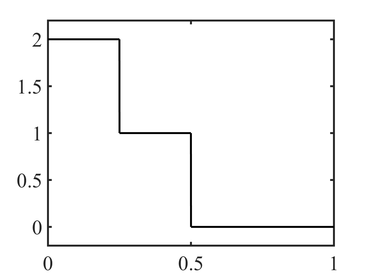
u0​(x)={2x<0.2510.25⩽x<0.50x⩾0.5.\displaystyle u_{0}(x)=\begin{cases}2&\quad x<0.25\\ 1&\quad 0.25\leqslant x<0.5\\ 0&\quad x\geqslant 0.5.\end{cases} (6.2)

We use the Godunov scheme, i.e. the monotone scheme (2.6) with Godunov flux function (3.14), and a CFL number of 0.30.3. The exact solution is

u⁡(x,t)={2x<0.25+1.5​t10.25+1.5​t⩽x<0.5+0.5​t0x⩾0.5+0.5​t\displaystyle u(x,t)=\begin{cases}2&\quad x<0.25+1.5t\\ 1&\quad 0.25+1.5t\leqslant x<0.5+0.5t\\ 0&\quad x\geqslant 0.5+0.5t\\ \end{cases}

for t<0.25t<0.25 and

u⁡(x,t)={2x<3/8+t0x⩾3/8+t\displaystyle u(x,t)=\begin{cases}2&\quad x<3/8+t\\ 0&\quad x\geqslant 3/8+t\\ \end{cases}

for t⩾0.25t\geqslant 0.25. At t=0.25t=0.25 the two shocks interact. The initial condition is plotted in Figure 2(a). In Figure 2(b)–(c) we see the exact solution and the numerical approximation before (t=0.15t=0.15) and after (t=0.3t=0.3) shock interaction. Tables 6.1 and 6.2 show the observed rate of convergence of the numerical approximation before and after the shock interaction; it is clear that the W1W_{1} error is O⁡(Δ​x2)O({\Delta x}^{2}), as claimed. The L1L^{1} error is O⁡(Δ​x)O({\Delta x}), as was shown in [16].

Refer to caption
(a) Initial condition.
Refer to caption
(b) Solution at t=0.15t=0.15.
Refer to caption
(c) Solution at t=0.3t=0.3.
Figure 2: The initial condition (6.2) and the exact solution (solid curve) and numerical approximation (dashed curve) of (6.1) before and after shock interaction. The color coding is the same as in Figure 1.
nn L1L^{1} L1L^{1} OOC W1W_{1} W1W_{1} OOC
3232 4.078×10−24.078\times 10^{-2} 1.775×10−31.775\times 10^{-3}
6464 2.735×10−22.735\times 10^{-2} 0.5770.577 6.523×10−46.523\times 10^{-4} 1.4451.445
128128 1.604×10−21.604\times 10^{-2} 0.7700.770 2.063×10−42.063\times 10^{-4} 1.6611.661
256256 8.478×10−38.478\times 10^{-3} 0.9200.920 5.699×10−55.699\times 10^{-5} 1.8561.856
512512 4.419×10−34.419\times 10^{-3} 0.9400.940 1.452×10−51.452\times 10^{-5} 1.9731.973
10241024 2.121×10−32.121\times 10^{-3} 1.0591.059 3.632×10−63.632\times 10^{-6} 1.9991.999
20482048 1.060×10−31.060\times 10^{-3} 1.0011.001 9.081×10−79.081\times 10^{-7} 2.0002.000
40964096 5.341×10−45.341\times 10^{-4} 0.9890.989 2.270×10−72.270\times 10^{-7} 2.0002.000
Table 6.1: Convergence rates for the Godunov scheme before the shock interaction, t=0.15t=0.15
nn L1L^{1} L1L^{1} OOC W1W_{1} W1W_{1} OOC
3232 2.848×10−22.848\times 10^{-2} 8.644×10−48.644\times 10^{-4}
6464 1.986×10−21.986\times 10^{-2} 0.5200.520 2.208×10−42.208\times 10^{-4} 1.9691.969
128128 6.780×10−36.780\times 10^{-3} 1.5501.550 3.955×10−53.955\times 10^{-5} 2.4812.481
256256 3.646×10−33.646\times 10^{-3} 0.8950.895 8.788×10−68.788\times 10^{-6} 2.1702.170
512512 1.176×10−31.176\times 10^{-3} 1.6321.632 1.892×10−61.892\times 10^{-6} 2.2152.215
10241024 9.863×10−49.863\times 10^{-4} 0.2540.254 5.291×10−75.291\times 10^{-7} 1.8381.838
20482048 3.710×10−43.710\times 10^{-4} 1.4111.411 1.182×10−71.182\times 10^{-7} 2.1632.163
40964096 2.255×10−42.255\times 10^{-4} 0.7180.718 3.308×10−83.308\times 10^{-8} 1.8371.837
Table 6.2: Convergence rates for the Godunov scheme after the shock interaction, t=0.3t=0.3

Tables 6.3 and 6.4 show the convergence rate of the second- and third-order ENO-schemes using third-order Runge-Kutta time integration and, in space, the Godunov flux with second- and third-order ENO reconstructions at the cell boundaries. Although the existence of discrete shocks has not been proven for higher-order schemes such as the second- and third-order ENO-schemes, we also observe a first-order convergence rate in the L1L^{1}-norm and a second-order rate in the W1W_{1}-distance, as shown in Tables 6.3 and 6.4.

nn L1L^{1} L1L^{1} OOC W1W_{1} W1W_{1} OOC
3232 2.125×10−22.125\times 10^{-2} 5.080×10−45.080\times 10^{-4}
6464 1.032×10−21.032\times 10^{-2} 1.0421.042 1.480×10−41.480\times 10^{-4} 1.7791.779
128128 5.307×10−35.307\times 10^{-3} 0.9600.960 3.824×10−53.824\times 10^{-5} 1.9531.953
256256 2.604×10−32.604\times 10^{-3} 1.0271.027 9.684×10−69.684\times 10^{-6} 1.9821.982
512512 1.492×10−31.492\times 10^{-3} 0.8040.804 2.432×10−62.432\times 10^{-6} 1.9941.994
10241024 6.553×10−46.553\times 10^{-4} 1.1871.187 5.965×10−75.965\times 10^{-7} 2.0272.027
20482048 3.319×10−43.319\times 10^{-4} 0.9810.981 1.496×10−71.496\times 10^{-7} 1.9951.995
40964096 1.628×10−41.628\times 10^{-4} 1.0281.028 3.783×10−83.783\times 10^{-8} 1.9841.984
Table 6.3: Convergence rates for the second-order ENO scheme with Godunov flux at t=0.15t=0.15
nn L1L^{1} L1L^{1} OOC W1W_{1} W1W_{1} OOC
3232 1.568×10−21.568\times 10^{-2} 3.454×10−43.454\times 10^{-4}
6464 6.516×10−36.516\times 10^{-3} 1.2671.267 8.128×10−58.128\times 10^{-5} 2.0872.087
128128 3.528×10−33.528\times 10^{-3} 0.8850.885 2.104×10−52.104\times 10^{-5} 1.9501.950
256256 1.696×10−31.696\times 10^{-3} 1.0561.056 5.286×10−65.286\times 10^{-6} 1.9931.993
512512 9.825×10−49.825\times 10^{-4} 0.7880.788 1.329×10−61.329\times 10^{-6} 1.9921.992
10241024 4.078×10−44.078\times 10^{-4} 1.2691.269 3.186×10−73.186\times 10^{-7} 2.0612.061
20482048 2.205×10−42.205\times 10^{-4} 0.8870.887 8.219×10−88.219\times 10^{-8} 1.9551.955
40964096 1.060×10−41.060\times 10^{-4} 1.0561.056 2.065×10−82.065\times 10^{-8} 1.9931.993
Table 6.4: Convergence rates for the third-order ENO scheme with Godunov flux at t=0.15t=0.15

7 Conclusion and outlook

With decreasing initial data consisting of a finite number of piecewise constants, we show that any monotone, W1W_{1}-contractive finite volume scheme will converge to the exact solution of (1.1) at a rate of Δ​x2{\Delta x}^{2} in the Wasserstein distance, both before and after shock interaction. The proof of the main result relies on the existence of discrete shocks and on the W1W_{1}-contractivity of the scheme. In Section 3.3 we show that the Lax–Friedrichs, Engquist–Osher and Godunov schemes are W1W_{1}-contractive, but a general result for all monotone schemes is ongoing work.

In addition to illustrating the main theorem in this paper, the numerical results in Section 6 show a second-order convergence rate in W1W_{1} for both the second- and third-order ENO schemes in the MUSCL formulation. Fan [4] has established existence of discrete shocks (for Dk​λD^{k}\lambda rational) for certain second-order MUSCL schemes. This suggests that it might be possible to prove existence of discrete shocks for a more general class of schemes and thus extend the main result of this paper.

Our analysis only applies to monotone schemes, and to an admittedly simple class of entropy solutions. Nonetheless, the main result, together with the numerical results for the higher-order ENO schemes, strongly suggest that measuring the approximation error in the W1W_{1}-distance may be the path to proving higher-order convergence rates. However, numerical evidence show that the O⁡(Δ​x)O(\Delta x) convergence rate obtained by Nessyahu, Tadmor and Tassa [9] is optimal for general Lip+\mathrm{Lip}^{+}-bounded initial data. Hence, it is necessary to use (formally) higher-order methods in order to tackle general initial data. The W1W_{1}-convergence rates of (formally) second- and higher-order schemes for more general initial data will be investigated further.

Finally, we mention that although the W1W_{1}-distance is easily defined also in several (spatial) dimensions, there are currently no results on the W1W_{1}-convergence of schemes for multi-dimensional conservation laws.

References

  • [1] B. Cockburn and P.-A. Gremaud. A priori error estimates for numerical methods for scalar conservation laws. Part I: The general approach. Math. Comp., 65:533–573, 1996.
  • [2] B. Enquist and S. Osher. One-side difference approximations for nonlinear conservation laws. Math. Comp., 36:321–351, 1981.
  • [3] H. Fan. Existence and uniqueness of traveling waves and error estimates for Godunov schemes of conservation laws. Math. Comp., 67:87–109, 1998.
  • [4] H. Fan. Existence of discrete shock profiles of a class of monotonicity preserving schemes for conservation laws. Math. Comp., 70:1043–1069, 2000.
  • [5] E. Godlewski and P.-A. Raviart. Hyperbolic systems of conservation laws. Ellipses, 1991.
  • [6] G. Jennings. Discrete Shocks. Comm. Pure Appl. Math., 27:25–37, 1974.
  • [7] N. N. Kuznetsov. Accuracy of some approximate methods for computing the weak solutions of a first-order quasi-linear equation. USSR Computational Mathematics and Mathematical Physics, 16(6):105–119, 1976.
  • [8] H. Nessyahu and E. Tadmor. The convergence rate of approximate solutions for nonlinear scalar conservation laws. SIAM J. Numer. Anal., 29:1505–1519, 1992.
  • [9] H. Nessyahu, E. Tadmor, and T. Tassa. The convergence rate of Godunov type schemes. SIAM J. Numer. Anal., 31:1–16, 1994.
  • [10] H. Nessyahu and T. Tassa. Convergence Rate of Approximate Solutions to Conservation Laws with Initial Rarefactions. SIAM J. Numer. Anal, 31:628–654, 1993.
  • [11] S. T. Rachev and R. M. Shortt. Duality theorems for Kantorovich-Rubinstein and Wasserstein functionals. Dissertationes Mathematicae, 299, 1990.
  • [12] F. Sabac. The Optimal Convergence Rate of Monotone Finite Difference Methods for Hyperbolic Conservation Laws. SIAM J. Numer. Anal., 34(6):2306–2318, 1997.
  • [13] D. Serre. L1-stability of nonlinear waves in scalar conservation laws. In C. Dafermos and E. Feireisl, editors, Handbook of Differential Equations. Evolutionary Equations, vol. 1. Elsevier, 2004.
  • [14] D. Serre. Discrete shock profiles: existence and stability. In P. Marcati, editor, Hyperbolic systems of balance laws. Springer-Verlag, 2007.
  • [15] E. Tadmor. Local Error Estimates for Discontinuous Solutions of Nonlinear Hyperbolic Equations. SIAM J. Numer. Anal., 28(4):891–906, 1991.
  • [16] Z.-H. Teng and P. Zhang. Optimal L1-Rate of Convergence for The Viscosity Method and Monotone Scheme to Piecewise Constant Solutions with Shocks. SIAM J. Numer. Anal., 34:959–978, 1997.
  • [17] C. Villani. Topics in Optimal Transportation. AMS, 2003.