A Spectral Series Approach to High-Dimensional Nonparametric Regression
Abstract
A key question in modern statistics is how to make fast and reliable inferences for complex, high-dimensional data. While there has been much interest in sparse techniques, current methods do not generalize well to data with nonlinear structure. In this work, we present an orthogonal series estimator for predictors that are complex aggregate objects, such as natural images, galaxy spectra, trajectories, and movies. Our series approach ties together ideas from manifold learning, kernel machine learning, and Fourier methods. We expand the unknown regression on the data in terms of the eigenfunctions of a kernel-based operator, and we take advantage of orthogonality of the basis with respect to the underlying data distribution, , to speed up computations and tuning of parameters. If the kernel is appropriately chosen, then the eigenfunctions adapt to the intrinsic geometry and dimension of the data. We provide theoretical guarantees for a radial kernel with varying bandwidth, and we relate smoothness of the regression function with respect to to sparsity in the eigenbasis. Finally, using simulated and real-world data, we systematically compare the performance of the spectral series approach with classical kernel smoothing, k-nearest neighbors regression, kernel ridge regression, and state-of-the-art manifold and local regression methods.
keywords
[class=MSC] 62G08keywords
high-dimensional inference, orthogonal series regression, data-driven basis, Mercer kernel, manifold learning, eigenmapsDepartment of Statistics, Carnegie Mellon University, USA.
??
Department of Statistics, Federal University of São Carlos, Brazil.
??
1 Introduction
A challenging problem in modern statistics is how to handle complex, high-dimensional data. Sparsity has emerged as a major tool for making efficient inferences and predictions for multidimensional data. Generally speaking, sparsity refers to a situation where the data, despite their apparent high dimensionality, are highly redundant with a low intrinsic dimensionality. In our paper, we use the term “sparse structure” to refer to cases where the underlying distribution places most of its mass on a subset of of small Lebesgue measure. This scenario includes, but is not limited to, Riemannian submanifolds of , and high-density clusters separated by low-density regions. In applications of interest, observable data often have (complex) sparse structure due to the nature of the underlying physical systems. For example, in astronomy, raw galaxy spectra are of dimension equal to the number of wavelength measurements , but inspection of a sample of such spectra will reveal clear, low-dimensional features and structure resulting from the shared physical system that generated these galaxies. While the real dimensionality of data is much smaller than , the challenge remains to exploit this when predicting, for example, the age, composition, and star formation history of a galaxy.
In its simplest form, low-dimensional structure is apparent in the original coordinate system. Indeed, in regression, much research on “large p, small n” problems concerns variable selection and the problem of recovering a “sparse” coefficient vector (i.e., a vector with mostly zeros) with respect to the given variables. Such approaches include, for example, lasso-type regularization [51], the Dantzig selector [9], and RODEO [28]. There are also various extensions that incorporate lower-order interactions and groupings of covariates [57, 61, 37] but, like lasso-type estimators, they are not directly applicable to the more intricate structures observed in, e.g., natural images, spectra, and hurricane tracks.
At the same time, there has been a growing interest in statistical methods that explicitly consider geometric structure in the data themselves. Most traditional dimension-reducing regression techniques, e.g., principal component regression (PCR; [26]) partial least squares (PLS; [55]) and sparse coding [35], are based on linear data transformations and enforce sparsity (with respect to the or norm) of the regression in a rotated space. More recently, several authors [7, 2, 10] have studied local polynomial regression methods on non-linear manifolds. For example, Aswani et al. [2] propose a geometry-based regularization scheme that estimates the local covariance matrix at a point and then penalizes regression coefficients perpendicular to the estimated manifold direction. In the same spirit, Cheng and Wu [10] suggest first reducing the dimensionality to the estimated intrinsic dimension of the manifold, and then applying local linear regression to a tangent plane estimate. Local regression and manifold-based methods tend to perform well when there is a clear submanifold but these approaches are not practical in higher dimensions or when the local dimension varies from point to point in the sample space. Hence, existing nonparametric models still suffer when estimating unknown functions (e.g., density and regression functions) on complex objects , where is large.
Much statistical research has revolved around adapting classical methods, such as linear, kernel-weighted, and additive models to high dimensions. On the other hand, statisticians have paid little attention to the potential of orthogonal series approaches. In low dimensions, orthogonal series is a powerful nonparametric technique for estimating densities and regression functions. Such methods are fast to implement with easily interpretable results, they have sharp optimality properties, and a wide variety of bases allows the data analyst to model multiscale structure and any challenging shape of the target function [16]. As a result, Fourier series approaches have dominated research in signal processing and mathematical physics. This success, however, has not translated to more powerful nonparametric tools in dimensions of the order of or ; in fact, extensions via tensor products (as well as more sophisticated adaptive grid or triangulation methods; see [31] and references within) quickly become unpractical in dimensions .
In this work, we will build on ideas from harmonic analysis and spectral methods to construct nonparametric methods for estimating unknown functions in high-dimensional spaces with non-standard data objects (such as images, spectra, and distributions) that possess sparse nonlinear structure. We derive a Fourier-like basis of that adapts to the intrinsic geometry of the underlying data distribution , and which is orthonormal with respect to rather than the Lebesgue measure of the ambient space. The empirical basis functions are then used to estimate functions on complex data ; such as, for example, the regression function of a response variable on an object . Because of the adaptiveness of the basis, there is no need for high-dimensional tensor products. Moreover, we take advantage of the orthogonality property of the basis for fast computation and model selection. We refer to our approach as spectral series as it is based on spectral methods (in particular, diffusion maps [13, 11, 29] and spectral connectivity analysis [30]) and Fourier series. Sections 2.1-2.3 describe the main idea of the series method in a regression setting.
Our work generalizes and ties together ideas in classical smoothing, kernel machine learning [44, 45, 14], support vector machines (SVMs; [49]) and manifold regularization [6] without the many restrictive assumptions (fixed kernel, exact manifold, infinite unlabeled data and so on) seen in other works. There is a large literature on SVMs and kernel machine learning that use similar approximation spaces as us, but it is unclear whether and how those procedures adapt to the structure of the data distribution. Generally, there is a discrepancy between theoretical work on SVMs, which assume a fixed RKHS (e.g., a fixed kernel bandwidth), and applied SVM work, where the RKHS is chosen in a data-dependent way (by, e.g., decreasing the kernel bandwidth for larger sample sizes ). Indeed, issues concerning the choice of tuning parameters, and their relation to the data distribution , are considered to be open problems in the mainstream RKHS literature. The manifold regularization work by Belkin et al. [6] addresses adaptivity to sparse structure but under restrictive assumptions, such as the existence of a well-defined submanifold and the presence of infinite unlabeled data.
Another key difference between our work and kernel machine learning is that we explicitly compute the eigenfunctions of a kernel-based operator and then use an orthogonal series approach to nonparametric curve estimation. Neither SVMs nor manifold regularizers exploit orthogonality relative to . In our paper, we point out the advantages of an orthogonal series approach in terms of computational efficiency (such as fast cross-validation and tuning of parameters), visualization, and interpretation. SVMs can sometimes have a “black box feel,” whereas the spectral series method allows the user to directly link the data-driven Fourier-like eigenfunctions to the function of interest and the sample space. Indeed, there is a dual interpretation of the computed eigenfunctions: (i) They define new coordinates of the data which are useful for nonlinear dimensionality reduction, manifold learning, and data visualization. (ii) They form an orthogonal Hilbert basis for functions on the data and are a means to nonparametric curve estimation via the classical orthogonal series method, even when there is no clearly defined manifold structure. There is a large body of work in the machine learning literature addressing the first perspective; see, e.g., Laplacian maps [3], Hessian maps [15], diffusion maps [13], Euclidean Commute Time maps [41], and spectral clustering [46]. In this paper, we are mainly concerned with the second view, i.e., that of estimating unknown functions on complex data objects and understanding the statistical properties of such estimators.
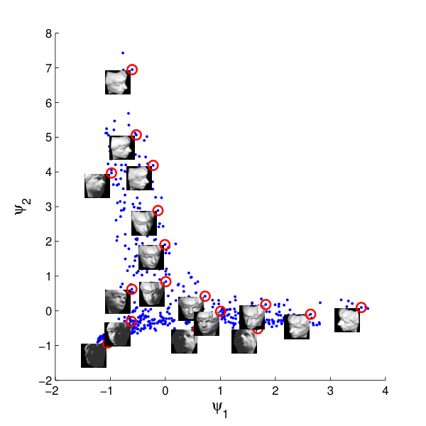
Fig. 1, for example, shows a 2D visualization of the Isomap face data using the eigenvectors of a renormalized Gaussian kernel as coordinates (Eq. 4). Assume we want to estimate the pose of the faces. How does one solve a regression problem where the predictor is an entire image? Traditional methods do not cope well with this task while our spectral series approach (Eq. 1 with estimated eigenfunctions as a basis) can use complex aggregate objects (e.g., images, spectra, trajectories, and text data) as predictors, without an explicit dimension reduction step. Note that the eigenvectors capture the pose and other continuous variations of an image fairly well, and that the regression appears to vary smoothly in sample space. We will return to the face pose estimation problem in Sec. 6.1. We will also discuss the theoretical properties of a spectral series estimator of the regression function in Sec. 5, including the connection between smoothness and efficient estimators.
Our paper has the following aims:
- (i)
Unifying. To generalize and connect ideas in kernel machine learning, manifold learning, spectral methods and classical smoothing, without the many restrictive assumptions (fixed kernel, exact manifold, infinite unlabeled data, low dimension) seen in other works.
- (ii)
Theoretical. To present new theoretical results in the limit of the kernel bandwidth that shed light on why RKHS/SVM methods often are so successful for complex data with sparse structure (Theorem 14 and Corollary 16), and to link smoothness of the regression with respect to to the approximation error of spectral series (Theorem 10).
- (iii)
Experimental. To systematically compare the statistical as well as the computational performance of spectral series and other methods using simulated and real-world data. Competing estimators include classical kernel smoothing, k-nearest neighbors (kNN) regression, regularization in RKHS, and recent state-of-the-art manifold and local regression methods. We ask questions such as: Do the methods scale well with increasing dimension and increasing sample size ? What is the estimated loss and what is the computational time?
The paper is organized as follows. In Sec. 2, we describe the construction of the spectral series method, including details on how to estimate relevant quantities from empirical data and how to tune model parameters. Sec. 3 discusses the connection to related work in machine learning and statistics. In Sections 4 and 5, we discuss the choice of kernel, and provide theoretical guarantees on the spectral series method. Finally, in Sec. 6, we compare the performance of spectral series and other nonparametric estimators for a wide variety of data sets.
2 Orthogonal Series Regression
2.1 General Formulation
In low dimensions, orthogonal series has proved to be a powerful technique for nonparametric curve estimation [16]. In higher dimensions, there is the question of whether one can find an appropriate basis and actually construct a series estimator that performs well. The general set-up of an orthogonal series regression is otherwise simple: Let be an iid sample from a distribution with compact support . Suppose we have a real-valued response
where is an unknown function, and denotes iid random noise with mean zero and variance . Our goal is to estimate the regression function in situations where is large and the data have sparse (i.e., low-dimensional) structure.
Let be an orthonormal basis of some appropriate Hilbert space with inner product and norm . We consider estimators of the form
| (1) |
where is a smoothing parameter, and and , in the general case, are data-based estimators of the basis functions and the expansion coefficients .
2.2 What Basis?
A challenging problem is how to choose a good basis. The standard approach in nonparametric curve estimation is to choose a fixed known basis for, say, , such as a Fourier or wavelet basis. There is then no need to estimate basis functions. In theory, such an approach can be extended to, eg., by a tensor product,11 1 Traditional orthogonal series estimators require tensor products in . For instance, if , then it is common to choose a basis of the form where , and and are bases for functions in . but tensor-product bases, as well as more sophisticated adaptive grid or triangulation methods (see [31] and references within), quickly become unusable for even as few as dimensions.
What basis should one then choose when the dimension is large, say, ? Ideally, the basis should be able to adapt to the underlying structure of the data distribution. This means: The basis should be orthogonal with respective to the distribution that generates the data, as opposed to the standard Lebesgue measure of the ambient space; the basis vectors should be concentrated around high-density regions where most of the “action” takes place; and the performance of the final series estimator should depend on the intrinsic rather than the ambient dimension of the data. In what follows, we present a spectral series approach where the unknown function is expanded into the estimated eigenfunctions of a kernel-based integral operator. As we shall see, the proposed estimator has many of the properties listed above.
2.3 Construction of Adaptive Basis
Our starting point is a symmetric and positive semi-definite (psd) so-called Mercer kernel . These kernels include covariance functions and polynomial kernels, but we are in this work primarily interested in local, radially symmetric kernels ,22 2 Depending on the application, one can replace the Euclidean distance with a dissimilarity measure that better reflects the distance between two data objects and . where is a parameter that defines the scale of the analysis, and the elements are positive and bounded for all . To simplify the theory, we renormalize the kernel according to
| (2) |
where . This normalization is common in spectral clustering because it yields eigenvectors that act as indicator functions of connected components [53, Section 3.2]. The same normalization is also implicit in traditional Nadaraya-Watson kernel smoothers, which compute the local average at a point by weighting surrounding points by .
We will refer to in Eq. 2 as the diffusion kernel. The term “diffusion” stems from a random walks view over the sample space [32, 30]: One imagines a Markov chain on with transition kernel . Starting at x, this chain moves to points close to , giving preference to points with high density . The chain essentially encodes the “connectivity” of the sample space relative to , and it has a unique stationary distribution given by
where as For finite , the stationary distribution is a smoothed version of .
In our regression setting, we seek solutions from a Hilbert space associated with the kernel . Following [30], we define a “diffusion operator” — which maps a function to a new function — according to
| (3) |
The operator has a discrete set of non-negative eigenvalues with associated eigenfunctions , which we for convenience normalize to have unit norm. These eigenfunctions have two very useful properties: First, they are orthogonal with respect to the density-weighted inner product
that is,
Second, they also form a set of oscillatory functions which are concentrated around high-density regions. By construction, is a constant function, and the higher-order eigenfunctions are increasingly oscillatory. Generally speaking, is the smoothest function relative to , subject to being orthogonal to for .
Interpretation. The diffusion operator and its eigenfunctions contain information about the connectivity structure of the sample space. There are two ways one can view the eigenfunctions :
- (i)
The eigenfunctions define new coordinates of the data. If the data represent high-dimensional complex objects, there is often no simple way of ordering the data. However, by a so-called “eigenmap”
(4) one can transform the data into an embedded space where points that are highly connected are mapped close to each other [29]. The eigenmap can be used for data visualization as in Fig. 1 and Fig. 6. If we choose , then we are effectively reducing the dimensionality of the problem by mapping the data from to .
- (ii)
The eigenfunctions form a Hilbert basis for functions on the data. More specifically, the set is an orthogonal basis of . The value of this result is that we can express most physical quantities that vary as a function of the data as a series expansion of the form .
In this work, we study the second point of view and its implications on nonparametric estimation in high dimensions.
2.4 Estimating the Regression Function from Data
In practice, of course, we need to estimate the basis and the projections from data. In this section, we describe the details.
Given , we compute a row-stochastic matrix , where
| (5) |
for . The elements can be interpreted as transition probabilities for a Markov chain over the data points (i.e., this is the discrete analogue of Eq. 2 and a diffusion over ). Let . The Markov chain has a unique stationary measure given by , where the th element
| (6) |
is a kernel-smoothed density estimate at the th observation.
To estimate the eigenfunctions of the continuous diffusion operator in Eq. 3, we first calculate the eigenvalues and the associated (orthogonal) eigenvectors of the symmetrized kernel matrix , where
| (7) |
We normalize the eigenvectors so that , and define the new vectors for and . By construction, it holds that the ’s and ’s are eigenvalues and right eigenvectors of the Markov matrix :
| (8) |
where
| (9) |
Note that the -dimensional vector can be regarded as estimates of at the observed values . In other words, let
| (10) |
for . We estimate the function at values of not corresponding to one of the ’s using the so-called Nyström method. The idea is to first rearrange the eigenfunction-eigenvalue equation as
and use the kernel-smoothed estimate
| (11) |
for .
Our final regression estimator is defined by Eq. 1 with the estimated eigenvectors in Eq. 11 and expansion coefficients computed according to
| (12) |
Remark 1 (Semi-Supervised Learning, SSL).
The spectral series framework naturally extends to semi-supervised learning (SSL) [60] where in addition to the “labeled” sample there are additional “unlabeled” data; i.e., data where the covariates but not the labels are known. Typically , as collecting data often is less costly than labeling them. By including unlabeled examples (drawn from the same distribution ) into the kernel matrix , we can improve our estimates of , and . The summation in Equations 9 and 11 will then be over all observations, while Eq. 12 remains the same as before. See e.g. [34, 58] for SSL with Laplacian eigenmaps in the limit of infinite unlabeled data, i.e., in the limit .
2.5 Loss Function and Tuning of Parameters
We measure the performance of an estimator via the loss function
| (13) |
To choose tuning parameters (such as the kernel bandwidth and the number of basis functions ), we split the data into a training and a validation set. For each choice of and a sufficiently large constant , we use the training set and Eqs. 11-12 to estimate the eigenvectors and the expansion coefficients . We then use the validation set to compute the estimated loss
| (14) |
for different values of . We choose the (, )-model with the lowest estimated loss on the validation set.
The computation for fixed and different is very fast. Due to orthogonality of the basis, the estimates and depend on but not on .
2.6 Scalability
The spectral series estimator is faster than most traditional approaches in high dimensions. Once the kernel matrix has been constructed, the eigendecomposition takes the same amount of time for all values of .
In terms of scalability for large data sets, one can dramatically reduce the computational cost by implementing fast approximate eigendecompositions. For example, the Randomized SVD by Halko et al. [22] cuts down the cost from to roughly with little impact on statistical performance (see Fig. 9). According to Halko et al., these randomized methods are especially well-suited for parallel implementation, which is a topic we will explore in future work.
3 Connection to Other Work
3.1 Linear Regression with Transformed Data
One can view our series model as a (weighted) linear regression after a data transformation , where are the first eigenvectors of the diffusion operator . By increasing , the dimension of the feature space, we achieve more flexible, fully nonparametric representations. Decreasing adds more structure to the regression, as dictated by the eigenstructure of the data.
Eq. 12 is similar to a weighted least squares (WLS) solution to a linear regression in but with an efficient orthogonal series implementation and no issues with collinear variables. Define the matrix of predictors,
| (15) |
and introduce the weight matrix
| (16) |
where and are estimated from data (Equations 6 and 10). Suppose that , where , , and the random vector represents the errors. By minimizing the weighted residual sum of squares
| (17) |
we arrive at the WLS estimator
| (18) |
where the matrix puts more weight on observations in high-density regions. This expression is equivalent to Eq. 12.
Note that thanks to the orthogonality property , model search and model selection are feasible even for complex models with very large . This is in clear contrast with standard multiple regression where one needs to recompute the estimates for each model with a different , invert the matrix , and potentially deal with inputs (columns of the design matrix ) that are linearly dependent.
Remark 2 (Heteroscedasticity).
More generally, let be a non-negative function rather than a constant, and let be iid realizations of a random variable with zero mean and unit variance. Consider the regression model . We can handle heteroscedastic errors by applying the same framework as above to a rescaled regression function .
3.2 Kernel Machine Learning and Regularization in RKHS
Kernel-based regularization methods use similar approximation spaces as us. In kernel machine learning [45, 14], one often considers the variational problem
| (19) |
where is a convex loss function, is a penalty parameter, and is the Reproducing Kernel Hilbert Space (RKHS) associated with a symmetric positive semi-definite kernel .33 3 To every continuous, symmetric, and positive semi-definite kernel is associated a unique RKHS [1]. This RKHS is defined to be the closure of the linear span of the set of functions with the inner product satisfying the reproducing property for all . Penalizing the RKHS norm imposes smoothness conditions on possible solutions. Now suppose that
where the RKHS inner product is related to the -inner product according to Eq. 19 is then equivalent to considering eigen-expansions
and seeking solutions to where the hypothesis space
| (20) |
is a ball of the RKHS with radius , and the RKHS norm is given by .
Here are some key observations:
(i) The above setting is similar to ours. The regularization in Eq. 19 differentially shrinks contributions from higher-order terms with small values. In spectral series, we use a projection (i.e., a basis subset selection) method, but the empirical performance is usually similar.
(ii) There are some algorithmic differences, as well as differences in how the two regression estimators are analyzed and interpreted. In our theoretical work, we consider Gaussian kernels with flexible variances; that is, we choose the approximation spaces in a data-dependent way (cf. multi-kernel regularization schemes for SVMs [56]) so that the estimator can adapt to sparse structure and the intrinsic dimension of the data. Most theoretical work in kernel machine learning assume a fixed RKHS.
(iii) There are also other differences. Support Vector Machines [49] and other kernel-based regularization methods (such as splines, ridge regression and radial basis functions) never explicitly compute the eigenvectors of the kernel. Instead, these methods rely on the classical Representer Theorem [54] which states that the solution to Eq. 19 is a finite expansion of the form . The original infinite-dimensional variational problem is then reduced to a finite-dimensional optimization of the coefficients . In a naive least-squares implementation, however, one has to recompute these coefficients for each choice of the penalty parameter , which can make cross-validation cumbersome. In our spectral series approach, we take advantage of the orthogonality of the basis for fast model selection and computation of the parameters. As in spectral clustering, we also use eigenvectors to organize and visualize data that can otherwise be hard to interpret.
3.3 Manifold Regularization and Semi-Supervised Learning
Our spectral series method is closely related to Laplacian-based regularization: In [6], Belkin et al. extend the kernel-based regularization framework to incorporate additional information about the geometric structure of the marginal . Their idea is to add a data-dependent penalty term to Eq. 19 that controls the complexity as measured by the geometry of the distribution. Suppose that one is given labeled data as well as unlabeled data , where in general . (The limit corresponds to having full knowledge of .) Under the assumption that the support of is a compact submanifold of , the authors propose minimizing a graph-Laplacian regularized least squares function
| (21) |
where are the edge weights in the graph, and the last Laplacian penalty term favors functions for which is close to when and are connected with large weights.
Note that the eigenbasis of our row-stochastic matrix minimizes the distortion in Eq. 21 if you regard the entries of as the weights [3]. Indeed, the eigenvector minimizes the term subject to being orthogonal to for . Hence, including a Laplacian penalty term is comparable to truncating the eigenbasis expansion in spectral series. Moreover, the semi-supervised regularization in Eq. 21 is similar to a semi-supervised version of our spectral series approach, where we first use both labeled and unlabeled data and a kernel with bandwidth to compute the eigenbasis, and then extend the eigenfunctions according to Eq. 11 via a (potentially wider) kernel with bandwidth . The main downside of the Laplacian-based framework above is that it is hard to analyze theoretically. As with other kernel-based regularizers, the method also does not explicitly exploit eigenvectors and orthogonal bases.
4 Choice of Kernel
In the RKHS literature, there is a long list of commonly used kernels. These include, e.g., the Gaussian kernel , polynomial kernels [52], and the thin-plate spline kernel [20]. In our numerical experiments (Sec. 6), we will consider both Gaussian and polynomial kernels, but throughout the rest of the paper, we will primarily work with the (row-normalized) Gaussian kernel. There are several reasons for this choice:
- (i)
- (ii)
The eigenfunctions of the Gaussian kernel are simultaneously concentrated in time (i.e., space) and frequency, and are particularly well-suited for estimating functions that are smooth with respect to a low-dimensional data distribution.
The following two examples illustrate some of the differences in the eigenbases of Gaussian and polynomial kernels:
Example 3.
Suppose that is a uniform distribution on the real line. Fig. 2, left, shows the eigenfunctions of a third-order polynomial kernel . These functions are smooth but have large values outside the support of . Contrast this eigenbasis with the eigenfunctions in Fig. 2, right, of a Gaussian kernel. The latter functions are concentrated on the support of and are orthogonal on as well as on .
Example 4.
Consider data around a noisy spiral:
where is a uniform random variable, and and are normally distributed random variables. The eigenfunctions of a polynomial kernel do not adapt well to the underlying distribution of the data. Fig. 3, left, for example, is a contour plot of the Nyström extension of the fourth empirical eigenvector of a third-order polynomial kernel. In contrast, the eigenfunctions of a Gaussian diffusion kernel vary smoothly along the spiral direction, forming a Fourier-like basis with orthogonal eigenfunctions that concentrate around high-density regions; see Fig. 3, right.
In high dimensions, Gaussian extensions can be seen as a generalization of prolate spheroidal wave functions [12]. Prolates were originally introduced by Slepian and Pollack as the solution to the problem of simultaneously and optimally concentrating a function and its Fourier content (see [48] for a fascinating recount of this development in Fourier analysis and modeling). The band-limited functions that maximize their energy content within a space domain are extensions of the eigenfunctions of the integral operator of a Bessel kernel restricted to [12, Section 3.1]. In high dimensions, Bessel and Gaussian kernels are equivalent [43], suggesting that the eigenfunctions of the Gaussian kernel are nearly optimal.
However, although Gaussian kernels have many advantages, they may not always be the best choice in practice. Ultimately, this is determined by the application and by what the best measure of similarity between two data points would be. Our framework suggests a principled way of selecting the best kernel for regression: Among a set of reasonable candidate kernels, choose the estimator with the smallest empirical loss according to Eq. 14. We will, for example, use this approach in Sec. 6 to choose the optimal degree for a set of polynomial kernels of the form .
Normalization of Local Kernels. In the RKHS literature, it is standard to work with “unnormalized” kernels. In spectral clustering [53], on the other hand, researchers often use the “stochastic” and “symmetric” normalization schemes in Eq. 5 and Eq. 7, respectively. We have found (Sec. 6) that the exact normalization often has little effect on the performance in regression. Nevertheless, we choose to use the row-stochastic kernel for reasons of interpretation and analysis: First, the limit of the bandwidth is well-defined, and there is a series of works on the convergence of the graph Laplacian to the Laplace-Beltrami operator on Riemannian manifolds [11, 5, 24, 47, 19]. Fourier functions originate from solving a Laplace eigenvalue problem on a bounded domain; hence, the eigenfunctions of the diffusion operator can be seen as a generalization of Fourier series to manifolds.
Moreover, the row-stochastic kernel yields less variable empirical functions than the unnormalized or symmetric forms. As an illustration, consider the noisy spiral data in Example 4. Fig. 4 shows the estimated projections onto the spiral direction of the eigenfunctions of the symmetric and the stochastic forms; see the left and right plots, respectively. The eigenfunctions are clearly smoother in the latter case. By construction, the empirical eigenfunctions of the symmetric operator are orthogonal with respect to the empirical distribution , whereas the estimated eigenfunctions of the stochastic operator are orthogonal with respect to the smoothed data distribution . The kernel bandwidth defines the scale of the analysis.
5 Theory
In this section, we derive theoretical bounds on the loss (Eq. 13) of a series regression estimator with a radial kernel for a standard fixed RKHS setting (Theorem 13), as well as a setting where the kernel bandwidth varies with the sample size (Theorem 14). We also further elaborate on the connection between spectral series and Fourier analysis by generalizing the well-known link between Sobolev differentiable signals and the approximation error in a Fourier basis.
Using the same notation as before, let
where and . We write
and refer to the two terms as “bias” and “variance”. Hence, we define the integrated bias and variance
and
and bound the two components separately. Our assumptions are:
(A1) has compact support and bounded density , .
(A2) The weights are positive and bounded; that is, ,
where and are constants that do not depend on .
(A3) The psd operator has nondegenerate eigenvalues; i.e.,
(A4) For all and , there exists some constant (not depending on ) such that
where and .
Without loss of generality, we assume that the eigenfunctions are estimated using an unlabeled sample that is drawn independently from the data used to estimate the coefficients . This is to simplify the proofs and can always be achieved by splitting the data in two sets.
5.1 Bias
A key point is that the approximation error of the regression depends on the smoothness of relative to . Here we present two different calculations of the bias based on two related notions of smoothness. The first notion is standard in the kernel literature and is based on RKHS norms. The second notion is based on our diffusion framework and can be seen as a generalization of Sobolev differentiability.
Method 1: Smoothness measured by RKHS norm.
Let where is a strictly positive number. Under previous assumptions, this kernel is symmetric and psd with a unique RKHS which we denote by . A standard way to measure smoothness of a function in a RKHS is through the RKHS norm (see, e.g., [33]). One can then define function classes
where is a positive number dependent on .
Proposition 5.
Assume , where . Then,
For fixed , contains “smoother” functions for smaller values of .
Method 2: Smoothness measured by diffusion operator.
Alternatively, let
| (22) |
where is the identity. The operator has the same eigenvectors as the differential operator . Its eigenvalues are given by where are the eigenvalues of . Define the functional
| (23) |
which maps a function into a non-negative real number. For small , measures the variability of the function with respect to the distribution . The expression is a variation of the graph Laplacian regularizers popular in semi-supervised learning [59]. In fact, a Taylor expansion yields where is the gradient operator and is the psd Laplace operator in . In kernel regression smoothing, the extra term is considered an undesirable extra bias, called design bias. In classical regression, it is removed by using local linear smoothing [17], which is asymptotically equivalent to replacing the original kernel by the bias-corrected kernel [11].
The following result bounds the approximation error of an orthogonal series expansion of . The bound is consistent with Theorem 2 in [58], which applies to the more restrictive setting of SSL with infinite unlabeled data and . Our result holds for all and and does not assume unlimited data.
Proposition 6.
For ,
| (24) | |||
where is the eigenvalue of .
Smoothness and Sparsity
In the limit , we have several interesting results, including a generalization of the classical connection between Sobolev differentiability and the error decay of Fourier approximations [31, Section 9.1.2] to a setting with adaptive bases and high-dimensional data. We denote the quantities derived from the bias-corrected kernel by , , and so forth.
Definition 7.
(Smoothness relative to P) A function is smooth relative to if
where is the stationary distribution of the random walk on the data as . The smaller the value of , the smoother the function.
Lemma 8.
For functions whose gradients vanish at the boundary,
This is similar to the convergence of the (un-normalized) graph Laplacian regularizer to the density-dependent smoothness functional [8].
Next we will see that smoothness relative to (Definition 7) and sparsity (with respect to the norm) in the eigenbasis of the diffusion operator (Definition 9 below) are really the same thing. As a result, we can link smoothness and sparsity to the rate of the error decay of the eigenbasis approximation.
Definition 9.
(Sparsity in ) A set of real numbers lies in a Sobolev ellipsoid if for some number . For a given basis , let
where . Functions in are sparse in . The larger the value of , the sparser the representation.
Theorem 10.
Assume that are the eigenvectors of with eigenvalues for some . Let . Then, the following two statements are equivalent:
- 1.
(smoothness relative to P)
- 2.
(sparsity in ).
Furthermore, sparsity in (or smoothness relative to P) implies
The rate of the error decay depends on the dimension of the data. We will address this issue in Sec. 5.3.
5.2 Variance
The matrix (defined in Eq. 5) can be viewed as a perturbation of the integral operator due to finite sampling. To estimate the variance, we bound the difference , where are the eigenvectors of , and are the Nyström extensions (Eq. 11) of the eigenvectors of . We adopt a strategy from Rosasco et al. [40], which is to introduce two new integral operators that are related to and but both act on an auxiliary44 4 This auxiliary space only enters the intermediate derivations and plays no role in the error analysis of the algorithm itself. RKHS of smooth functions (see Appendix A.2 for details). As before, we write to indicate that we let the kernel bandwidth depend on the sample size .
Proposition 11.
Let and as . Under assumptions (A1)-(A4) and ,
where and
Proposition 12.
Let and . Under (A1)-(A4) and for , it holds that
where .
5.3 Total Loss
Fixed Kernel
In kernel machine learning, it is standard to assume a fixed RKHS , e.g., with norm and a fixed kernel with a bandwidth not dependent on . From Propositions 5 and 12 and under assumptions (A1)-(A4), we then have the following result:
Theorem 13.
Assume with finite norm; i.e., for some constant . Then,
| (25) |
where .
The problem is that , , and the eigenvalues , all depend on . This dependence is complicated and poorly understood. Hence, in what follows, we will instead of the RKHS norm use an alternative measure of smoothness based on the diffusion operator (Method 2 in Sec. 5.1). This simplifies the theory and will allow us to analyze the dependence of the series estimator on tuning parameters and sparse structure.
Kernel with Decreasing Bandwidth
Consider now a Gaussian kernel with a bandwidth that decreases with increasing . From Propositions 6 and 12 and under assumptions (A1)-(A4), we have the following results:
Theorem 14.
Let and as . Then, for ,
| (26) |
where , is the eigenvalue of , , and .
Corollary 15.
Assume that and that the kernel is corrected for bias. Then, for and ,
| (27) |
where is the eigenvalue of , , and .
Some comments on these results: The first term in Eqs. 25-27 corresponds to the approximation error of the estimator and decays with . The second and third terms correspond to the variance. Note that the variance term is the same as the variance of a traditional orthogonal series estimator in one dimension only; in dimensions, the variance term for a traditional tensor product basis is where is the number of components in the th direction [16]. Hence, there is a considerable gain in using an adaptive bias, but we incur an additional variance term from estimating the basis.55 5 In an SSL setting (Remark 1), this extra estimation error vanishes in the limit of infinite unlabeled data.
If we balance the two -terms in Eq. 27, we get a bandwidth of . With this choice of and by ignoring terms of lower order, the rate becomes
| (28) |
Finally, if we apply the results in [11, 18, 19, 40] to general Riemannian manifolds (see, for example, [25, 36, BerrySauer:2016] for kernel density estimation on manifolds), and use that the eigenvalues of the Laplace-Beltrami operator on an -dimensional Riemannian manifold are [42], we obtain the following corollary:
Corollary 16.
We make the following observations for a spectral series estimator with flexible kernel bandwidth:
- (i)
Adaptiveness to Low-Dimensional Structure. If the data in has intrinsic dimension , then the rate above is a significant improvement of the minimax rate for a nonparametric regressor in . Our estimator automatically adapts to sparse structure and does not require the knowledge of or an estimated in practice. The optimal error rate is achieved when the smoothing parameters and are properly selected for the given , and the amount of smoothing is in practice chosen by cross-validation as in Sec. 2.5.
- (ii)
Minimax Optimality. In a semi-supervised learning setting, the estimation error of the basis vanishes in the limit of infinite unlabeled data. The loss then reduces to
(29) which is minimized by taking . At the minimum, we achieve the rate
the minimax rate for a nonparametric estimator of Sobolev smoothness in , where . The latter result is also, up to a logarithmic term, in agreement with [58].
6 Numerical Examples
Finally, we use data with complex dependencies to compare the spectral series approach with classical kernel smoothing, k-nearest neighbors (kNN) regression, regularization in RKHS, and recent state-of-the-art manifold and local regression methods.
In our experiments, we split the data into three sets for training, validation, and testing, respectively. For the manifold regression estimators from Aswani et al [2] and Cheng et al. [10], we use the authors’ codes with built-in cross-validation. For all other estimators, we tune parameters according to Sec. 2.5. To assess the final models, we compute the estimated loss and standard error on the test data.66 6 The estimated standard error of is , where is the empirical variance of on the test set.
6.1 Estimating Pose Using Images of Faces
In our first example, we consider images of artificial faces from the Isomap database [50].77 7 www.isomap.stanford.edu/datasets.html There are a total of gray-scale images rendered with different orientation and lighting directions. Fig. 1 shows a visualization of these data where we use the first two non-trivial eigenvectors of the Gaussian diffusion kernel as coordinates (i.e., Eq. 4 with the approximate eigenvectors from Eq. 11).
Our goal is to estimate the horizontal left-right pose of each face. We compare several different approaches to regression:
(i) As a baseline, we choose the classical Nadaraya-Watson estimator with a Gaussian smoothing kernel (NW) and the k-nearest neighbors regression estimator (kNN). The latter estimator is known to be minimax optimal with respect to local intrinsic dimension [27].
(ii) For the spectral series method (Series), we implement the Gaussian kernel (Series-radial) and polynomial kernels of different degrees . We treat as a tuning parameter and we denote the polynomial kernel with the smallest estimated loss by Series-polyBest. Note that choosing (Series-poly1) is equivalent to a linear regression on eigenvectors computed with PCA.
(iii) We also implement the RKHS method in Sec. 3.2 for the same set of kernels as Series. For a squared-error loss, Eq. 19 reduces to an infinite-dimensional, generalized ridge regression problem [23, Section 5.8.2]. Hence, we use the term kernel ridge regression (KRR) and denote the estimators by KRR-radial and KRR-poly.
(iv) The last group of estimators include recent manifold and local regression methods [2, 10]88 8 For code, go to www.eecs.berkeley.edu/~aaswani/EDE_Code.zip and http://www.math.princeton.edu/~hauwu/regression.zip.: locOLS is a local ordinary least squares, locRR is a local ridge regression, locEN is a local elastic net, locPLS is a local partial least squares, locPCR is a local principal components regression, NEDE is the nonparametric exterior derivative estimator, NALEDE is the nonparametric adaptive lasso exterior derivative estimator, NEDEP is the nonparametric exterior derivative estimator for the “large p, small n” case, and NALEDEP is the nonparametric adaptive lasso exterior derivative estimator for the “large p, small n” case. The last 4 regression estimators (NEDE, NALEDE, NEDEP, NALEDP) pose the regression as a least-squares problem with a term that penalizes for the regression vector lying in directions perpendicular to an estimated manifold; see [2] for details. In our comparison, we also include MALLER [10] which first estimates the local dimension of the data and then performs local linear regression on a tangent plane estimate.
Manifold and local regression methods, unlike Series, quickly become computationally intractable in high dimensions. Hence, to be able to compare the different methods, we follow Aswani et al. [2] and rescale the Isomap images from from down to pixels in size. This reduces the number of covariates from to . In other words, we regress the left-right pose (our response) on the rescaled image (our predictor). We use 50% of the data for training, 25% for validation and 25% for testing. All covariates are normalized to have mean 0 and standard deviation 1.
Table 1 and Fig. 5 summarize the results of the final (cross-validated) estimators. The approaches that have best performance are Series-radial and KRR-radial. As expected, Series and KRR estimators yield similar losses. A first-order polynomial kernel, i.e., a global principal component regression with Series- or KRR-poly1, performs worse than NW and kNN. Higher-order polynomial kernels (with degree resulting in the smallest loss) as well as the manifold and local regression estimators (in particularly, NEDE and MALLER) improve the NW and kNN results but Series-radial and KRR-radial are still the best choices in terms of statistical and computational performance.
| Method | Loss (SE) |
|---|---|
| NW | 1.71 (0.23) |
| kNN | 1.74 (0.21) |
| Series-poly1 | 2.96 (0.40) |
| Series-polyBest (q=2) | 0.22 (0.04) |
| Series-radial | 0.16 (0.04) |
| KRR-poly1 | 2.95 (0.41) |
| KRR-polyBest (q=2) | 0.22 (0.05) |
| KRR-radial | 0.15 (0.04) |
| Method | Loss (SE) |
|---|---|
| locOLS | 0.65 (0.17) |
| locRR | 0.46 (0.16) |
| locEN | 0.47 (0.16) |
| locPLS | 0.65 (0.21) |
| locPCR | 0.95 (0.20) |
| NEDE | 0.44 (0.14) |
| NALEDE | 0.46 (0.14) |
| NEDEP | 0.81 (0.31) |
| NALEDEP | 0.85 (0.33) |
| MALLER | 0.24 (0.06) |
6.2 Estimating Redshift Using SDSS Galaxy Spectra
In the following (high-dimensional) example, we predict the redshift of galaxies from high-resolution measurements of their emission spectra. Our initial data sample consists of galaxy spectra from ten arbitrarily chosen spectroscopic plates of SDSS DR6.99 9 http://www.sdss.org/dr6/algorithms/redshift_type.html We preprocess and remove spectra according to the three cuts described in [38]. The final sample consists of high-resolution spectra with flux measurements at wavelengths. We renormalize each spectra so that it has unit norm. Our goal is to predict a galaxy’s redshift where the predictor is an entire spectrum . Fig. 6a shows an example of a SDSS spectrum. Fig. 6b shows a low-dimensional visualization of the full data set when using the first few vectors of the diffusion basis as coordinates. Each point in the plot represents a galaxy, and the color codes for the SDSS spectroscopic redshift. The redshift (the response ) appears to vary smoothly with the eigencoordinates.
For the regression, we use 50% of the data for training, 25% for validation and 25% for testing. Due to the high dimension of the predictor (), we are unable to implement the computationally intensive manifold and local regression estimators from [2]. Table 2 and Fig. 7 summarize the results for the other approaches to regression. Series and KRR are essentially equivalent in terms of performance, and as before, the radial kernel (Series-radial and KRR-radial) yields the smallest estimated loss. For these data, a linear dimensionality reduction with PCA (series-poly1) improves upon the NW and kNN regression results. MALLER and higher-order polynomials (with degrees 5 and 6) perform better than PCA, but Series-radial still has the smallest estimated loss. Moreover, MALLER is much slower than Series: the former estimator takes 34 minutes on a 2.70GHz Intel Core i7-4800MQ, whereas Series with cross-validation takes less than a minute.
| Method | Loss (SE) |
|---|---|
| NW | 6.13 (1.47) |
| kNN | 6.37 (1.52) |
| Series-poly1 | 5.13 (0.47) |
| Series-polyBest (q=5) | 3.22 (0.32) |
| Series-radial | 2.77 (0.33) |
| KRR-poly1 | 5.01 (0.49) |
| KRR-polyBest (q=6) | 3.05 (0.33) |
| KRR-radial | 2.84 (0.33) |
| Method | Loss (SE) |
|---|---|
| locOLS | – |
| locRR | – |
| locEN | – |
| locPLS | – |
| locPCR | – |
| NEDE | – |
| NALEDE | – |
| NEDEP | – |
| NALEDEP | – |
| MALLER | 3.11 (0.38) |
6.3 Scalability
Increasing Dimension
In terms of computational speed, the spectral series estimator has a clear competitive edge in high dimensions relative local regression procedures and a least-squares (LS) implementation of Eq. 19 that does not take advantage of orthogonal bases (see, e.g., [4, p. 215] for a LS implementation of SSL learning on manifolds). We illustrate the differences with a one-dimensional manifold embedded in dimensions. Let where the points lie on a unit circle in , and is the angle corresponding to the position of . For simplicity, we simulate data uniformly on the circle; i.e., we let .
Figure 8 summarizes the results. In terms of estimated loss (left panel), Series performs better than MALLER, and it has a statistical performance similar to the least-squares implementation of kernel ridge regression (KRR-LS). As predicted by the theory, the loss of Series does not depend on the ambient dimension . Moreover, the computational time of Series is nearly constant as a function of the dimension (right panel). KRR-LS is slower than Series,1010 10 Cross-validation of Series is fast due to the orthogonality of the basis. If we compute the expansion coefficients (Eq. 12) for all , then we do not need to recompute these coefficients for other models with the same kernel and components in the series expansion. The least squares implementation of Eq. 19, on the other hand, requires recomputing the expansion coefficients for each choice of the smoothing parameter . and MALLER becomes computationally intractable as increases. For and , each fit with MALLER takes an average of 354 seconds (6 minutes) on an Intel i7-4800MQ CPU 2.70GHz processor, compared to 72 seconds for Series.
Increasing Sample Size
Here we revisit the redshift prediction problem in Sec. 6.2 using galaxy spectra from SDSS DR 12.1111 11 http://www.sdss.org/dr12/ We increase the size of the training set for a fixed number of validation spectra and test spectra. Fig. 9 indicates massive payoffs in implementing Randomized SVD (Series RSVD) for large data sets; see discussion in Sec. 2.6. Even without parallelization, we are able to cut down the computational time with a factor of 15 (right panel) with almost no decrease in statistical performance (left panel). The run time for SVD and KRR-LS when the sample size n=11200 (and the dimension ) is about 5 hours on an Intel i7-4800MQ CPU 2.70GHz processor. With Randomized SVD, the same regression takes about 20 minutes.
7 Discussion
Our spectral series method can handle complex high-dimensional data objects in many settings where traditional nonparametric methods either perform poorly or are computationally intractable. The series method offers a compression of the data in terms of Fourier coefficients; it is computationally efficient (with regards to the dimension and size of the sample), and it returns orthogonal basis functions that adapt to low-dimensional structure in the data distribution. As a result, there is no need for cumbersome tensor products in high dimensions.
Our work shows that for a Gaussian kernel with a flexible bandwidth, the computed eigenfunctions form a Fourier-like orthogonal basis for expressing smoothness relative to the underlying data distribution. More precisely, if a function is smooth with respect to the data distribution, then it is sparse in the eigenbasis with respect to the norm, and vice versa (Theorem 10). Indeed, in the limit of the sample size , spectral series with a Gaussian kernel can be seen as a generalization of Fourier series to high dimensions and sparse structure (Sec. 4).
The two main theorems 13 and 14 provide theoretical bounds on the loss of the final regression estimator for a standard fixed RKHS setting as well as a setting where the kernel bandwidth varies with the sample size . We show that spectral series regression with a Gaussian kernel is adaptive to intrinsic dimension when the bandwidth (Corollary 16). In the case of a submanifold with dimension embedded in , the convergence rate of the estimator depends on the manifold dimension rather than the ambient dimension . The adaption occurs automatically and does not involve manifold estimation. Unlike [7], there is also no need to estimate the dimension of the manifold. We have found that unless the goal is manifold estimation, there is little advantage in using manifold and local linear regression methods. Such methods quickly become computationally intractable in high dimensions without a prior dimension reduction. On the other hand, the computational speed of spectral series does not depend on the ambient or intrinsic dimension of the data. Moreover, it is unclear how manifold-based methods behave in more complex settings where there is sparse structure (e.g., high-density regions and clusters) but no well-defined submanifold.
Because of the close connection between spectral series and SVMs, we expect that our new findings (regarding adaptiveness, choice of kernel and the bandwidth) will apply to kernel-based regularized empirical risk minimizers as well. Indeed, our empirical results (Tables 1 and 2) confirm that the performance of KRR using a Gaussian kernel with a flexible bandwidth is similar to that of spectral series regression. This suggests that one can exploit the advantages of spectral series in terms of interpretation, visualization, and analysis without any real down-sides. In the process of analyzing the performance of the spectral series estimator, we shed light on the empirical success of SVMs for sparse data, and we unify ideas from Fourier analysis, kernel machine learning and spectral clustering.
Future work includes deriving tighter bounds for the convergence rate of spectral series and kernel-based empirical regularizers. We believe that our estimated rates are on the conservative side as our derivations assume that the eigenvectors need to be accurately estimated. Empirical experiments, however, indicate that spectral series with approximate eigenvectors already outperform the -nearest neighbor estimator which is minimax optimal with respect to local intrinsic dimension [27]. In a separate paper, we will discuss extensions of spectral series to estimating other unknown functions (e.g., conditional densities, density ratios and likelihoods) for high-dimensional complex data and distributions. Another interesting research question is whether one can further improve the performance of spectral series approaches by adaptive basis selection and nonlinear estimators that threshold the series expansion coefficients as in wavelet thresholding [31].
In the online supplementary materials, we include sample R code for the spectral series estimator. This code has however not been optimized for speed, as we will leave the large-scale deployment on parallel platforms to future work.
8 Acknowledgments
We are grateful to Ronald R. Coifman and Larry Wasserman for the original discussions that led to this work. We would also like to thank Peter Freeman, Cosma Shalizi and Ryan Tibshirani for insightful comments on the manuscript. This work was partially supported by the Estella Loomis McCandless Professorship, Conselho Nacional de Desenvolvimento Científico e Tecnológico (grant 200959/2010-7), Fundação de Amparo à Pesquisa do Estado de São Paulo (2014/25302-2), and NSF DMS-1520786.
References
- [1] Aronszajn, N. (1950). Theory of reproducing kernels. Transactions of the American Mathematical Society 68(3), 337–404.
- [2] Aswani, A., P. Bickel, and C. Tomlin (2011). Regression on manifolds: Estimation of the exterior derivative. Annals of Statistics 39(1), 48–81.
- [3] Belkin, M. and P. Niyogi (2003). Laplacian eigenmaps for dimensionality reduction and data representation. Neural Computation 6(15), 1373–1396.
- [4] Belkin, M. and P. Niyogi (2005a). Semi-supervised learning on Riemannian manifolds. Machine Learning 56, 209–239.
- [5] Belkin, M. and P. Niyogi (2005b). Towards a theoretical foundation for Laplacian-based manifold methods. In Proc. Conf. on Learning Theory, Volume 3559, pp. 486–500.
- [6] Belkin, M., P. Niyogi, and V. Sindhwani (2006). Manifold regularization: A geometric framework for learning from labeled and unlabeled examples. Journal of Machine Learning Research 7, 2399–2434.
- [7] Bickel, P. J. and B. Li (2007). Local polynomial regression on unknown manifolds. In IMS Lecture Notes–Monograph Series, Complex Datasets and Inverse Problems, Volume 54, pp. 177–186. Institute of Mathematical Statisitcs.
- [8] Bousquet, O., O. Chapelle, and M. Hein (2003). Measure based regularization. In Adv. in Neural Inf. Processing Systems.
- [9] Candès, E. and T. Tao (2005). The Dantzig selector: statistical estimation when p is much larger than n. Ann. Stat..
- [10] Cheng, M. Y. and H. T. Wu (2013). Local linear regression on manifolds and its geometric interpretation. Journal of the American Statistical Association 108, 1421–1434.
- [11] Coifman, R. and S. Lafon (2006a). Diffusion maps. Applied and Computational Harmonic Analysis 21, 5–30.
- [12] Coifman, R. and S. Lafon (2006b). Geometric harmonics. Applied and Computational Harmonic Analysis 21, 31–52.
- [13] Coifman, R., S. Lafon, A. Lee, M. Maggioni, B. Nadler, F. Warner, and S. Zucker (2005). Geometric diffusions as a tool for harmonics analysis and structure definition of data: Diffusion maps. Proc. of the National Academy of Sciences 102(21), 7426–7431.
- [14] Cucker, F. and D. Zhou (2007). Learning Theory: An Approximation Theory Viewpoint. Cambridge University Press.
- [15] Donoho, D. and C. Grimes (2003, May). Hessian eigenmaps: new locally linear embedding techniques for high-dimensional data. Proc. of the National Academy of Sciences 100(10), 5591–5596.
- [16] Efromovich, S. (1999). Nonparametric Curve Estimation: Methods, Theory and Application. Springer.
- [17] Fan, J. (1993). Local linear regression smoothers and their minimax efficiencies. Annals of Statistics 21, 196–216.
- [18] Giné, E. and A. Guillou (2002). Rates of strong uniform consistency for multivariate kernel density estimators. Ann Inst. H. Poincar 38, 907–921.
- [19] Giné, E. and V. Koltchinskii (2006). Empirical graph Laplacian approximation of Laplace-Beltrami operators: Large sample results. In High Dimensional Probability: Proceedings of the Fourth International Conference, IMS Lecture Notes, pp. 1–22.
- [20] Girosi, F., M. Jones, and T. Poggio (1995). Regularization theory and neural network architectures. Neural Computation 7, 219–269.
- [21] Grigor’yan, A. (2006). Heat kernels on weighted manifolds and applications. Cont. Math. 398, 93–191.
- [22] Halko, N., P. G. Martinsson, and J. A. Tropp (2011). Finding structure with randomness: Probabilistic algorithms for constructing approximate matrix decompositions. SIAM Review 53(2), 217–288.
- [23] Hastie, T., R. Tibshirani, and J. Friedman (2009). The Elements of Statistical Learning (Second ed.). Springer.
- [24] Hein, M., J.-Y. Audibert, and U. von Luxburg (2005). Intrinsic dimensionality estimation of submanifolds in . In Proc. of the 22nd Int’l Conf on Machine learning.
- [25] Henry, G. and D. Rodriguez (2009). Kernel density estimation on riemannian manifolds: Asymptotic results. Journal of Mathematical Imaging and Vision 34(3), 235–239.
- [26] Jolliffe, I. T. (2002). Principal Component Analysis. Springer.
- [27] Kpotufe, S. (2011). k-NN regression adapts to local intrinsic dimension. In Advances in Neural Information Processing Systems 24, pp. 729–737. The MIT Press.
- [28] Lafferty, J. and L. Wasserman (2008). Rodeo: Sparse, greedy nonparametric regression. Annals of Statistics 36(1), 28–63.
- [29] Lafon, S. and A. Lee (2006). Diffusion maps and coarse-graining: A unified framework for dimensionality reduction, graph partitioning, and data set parameterization. IEEE Trans. Pattern Anal. and Mach. Intel. 28, 1393–1403.
- [30] Lee, A. and L. Wasserman (2010). Spectral connectivity analysis. Journal of the American Statistical Association 105(491), 1241–1255.
- [31] Mallat, S. (2009). A Wavelet Tour of Signal Processing (3rd ed.). Academic Press.
- [32] Meila, M. and J. Shi (2001). A random walks view on spectral segmentation. In Proc. Eighth International Conference on Artificial Intelligence and Statistics.
- [33] Minh, H. Q., P. Niyogi, and Y. Yao (2006). Mercer’s theorem, feature maps, and smoothing. In Learning Theory, 19th Annual Conference on Learning Theory.
- [34] Nadler, B., A. Srebro, and X. Zhou (2009). Semi-supervised learning with the graph laplacian: The limit of infinite unlabelled data.
- [35] Olshausen, B. A. and D. J. Field (1996). Emergence of simple-cell receptive field properties by learning a sparse code for natural images. Nature 381(6583), 607–609.
- [36] Ozakin, A. and A. Gray (2009). Submanifold density estimation. In Adv. in Neural Inf. Processing Systems, pp. 1375–1382.
- [37] Ravikumar, P., J. Lafferty, H. Liu, and L. Wasserman (2009). Sparse additive models. Journal of the Royal Statistical Society, Series B 71(5), 1009–1030.
- [38] Richards, J. W., P. E. Freeman, A. B. Lee, and C. M. Schafer (2009). Exploiting low-dimensional structure in astronomical spectra. Astrophysical Journal 691, 32–42.
- [39] Rosasco, L., M. Belkin, and E. D. Vito (2008). A note on perturbation results for learning empirical operators. CSAIL Technical Report TR-2008-052, CBCL-274, Massachusetts Institute of Technology.
- [40] Rosasco, L., M. Belkin, and E. D. Vito (2010). On learning with integral operators. Journal of Machine Learning Research 11, 905–934.
- [41] Saerens, M., F. Fouss, L. Yen, and P. Dupont (2004). The principal components analysis of a graph, and its relationships to spectral clustering. In Proceedings of the 15th European Conference on Machine Learning (ECML 2004). Lecture Notes in Artificial Intelligence, pp. 371–383. Springer-Verlag.
- [42] Safarov, Y. and D. Vassiliev (1996). The Asymptotic Distribution of Eigenvalues of Partial Differential Operators, Volume 155 of Translations of Mathematical Monographs. American Mathematical Society.
- [43] Schoenberg, I. J. (1938). Metric spaces and completely monotone functions. Annals of Mathematics 39(4), 811–841.
- [44] Schölkopf, B., A. Smola, and K. R. Müller (1997). Kernel principal component analysis. In Artificial Neural Networks - ICANN’97, pp. 583–588. Springer.
- [45] Schölkopf, B. and A. J. Smola (2001). Learning with Kernels. MIT Press.
- [46] Shi, T., M. Belkin, and B. Yu (2009). Data spectroscopy: Eigenspaces of convolution operators and clustering. The Annals of Statistics 37(6B), 3960–3984.
- [47] Singer, A. (2006). From graph to manifold Laplacian: The convergence rate. Applied and Computational Harmonic Analysis 21, 128–134.
- [48] Slepian, D. (1983). Some comments on fourier analysis, uncertainty and modeling. SIAM Review 25(3), 379–393.
- [49] Steinwart, I. and A. Christmann (2008). Support Vector Machines. Springer.
- [50] Tenenbaum, J. B., V. de Silva, and J. C. Langford (2000). A Global Geometric Framework for Nonlinear Dimensionality Reduction. Science 290(5500), 2319–2323.
- [51] Tibshirani, R. (1996). Regression shrinkage and selection via the lasso. Journal of the Royal Statistical Society, Series B, Methodological 58, 267–288.
- [52] Vapnik, V. (1996). Statistical Learning Theory. Wiley.
- [53] von Luxburg, U. (2007). A tutorial on spectral clustering. Statistics and Computing 17(4), 395–416.
- [54] Wahba, G. (1990). Spline Models for Observational Data. SIAM.
- [55] Wold, S., M. Sjöström, and L. Eriksson (2001). PLS-regression: a basic tool of chemometrics. Chemometrics and intelligent laboratory systems 58, 109–130.
- [56] Wu, Q., Y. Ying, and D.-X. Zhou (2007). Multi-kernel regularized classifiers. Journal of Complexity 23, 108–134.
- [57] Yuan, M. and Y. Lin (2006). Model selection and estimation in regression with grouped variables. Journal of the Royal Statistical Society, Series B 68(1), 49–67.
- [58] Zhou, X. and N. Srebro (2011). Error analysis of Laplacian eigenmaps for semi-supervised learning. In Proceedings of the Fourteenth International Conference on Artificial Intelligence and Statistics, Volume 15, pp. 892–900.
- [59] Zhu, X., Z. Ghahramani, and J. Lafferty (2003). Semi-supervised learning using gaussian fields and harmonic functions. In ICML-03, 20th International Conference on Machine Learning.
- [60] Zhu, X. and A. B. Goldberg (2009). Introduction to semi-supervised learning. Synthesis lectures on artificial intelligence and machine learning 3(1), 1–130.
- [61] Zou, H. and T. Hastie (2005). Regularization and variable selection via the elastic net. Journal of the Royal Statistical Society, Series B 67(2), 301–320.
A Proofs for Bounds on the Regression Estimator
We start by stating some useful lemmas.
Lemma 17.
[11, Proposition 3] For and ,
If is a compact submanifold of , then is the psd Laplace-Beltrami operator of defined by , where are the normal coordinates of the tangent plane at .
Lemma 18.
,
Proof.
,
where . ∎
Lemma 19.
For ,
Proof.
From the orthogonality property of the basis functions , we have that
The result follows from Lemma 18. ∎
Lemma 20.
Proof.
Lemma 21.
, it holds that
Proof.
Let and . According to Chebyshev’s inequality, for any ,
Hence, for any ,
where we in the last inequality apply the Cauchy-Schwarz inequality. Under assumption (A4), we conclude the result of the lemma. ∎
A.1 Bias
Proof of Proposition 5. Let be the eigenfunctions of the symmetric operator . It follows from Mercer’s theorem that
If , then we can bound the bias with respect to the eigenbasis :
By construction,
and
Thus,
The result follows from Lemma 19.
A.2 Variance
Let be an auxiliary RKHS of smooth functions; we use the term “auxiliary” to denote that the space only enters the intermediate derivations and plays no role in the error analysis of the algorithm itself. We define the two integral operators where
and is the reproducing kernel of . Define the operator norm where . Now suppose the weight function is sufficiently smooth with respect to (Assumption 1 in [40]); this condition is for example satisfied by a Gaussian kernel on a compact support . By Propositions 13.3 and 14.3 in [40], we can then relate the functions and , respectively, to the eigenfunctions and of and . We have that
| (30) |
for some constants and . According to Theorem 6 in [39] for eigenprojections of positive compact operators, it holds that
| (31) |
where is proportional to the eigengap . As a result, we can bound the difference by controlling the deviation .
We choose the auxiliary RKHS to be a Sobolev space with a sufficiently high degree of smoothness (see below for details). Let denote the Sobolev space of order with vanishing gradients at the boundary; that is, let
where is the weak partial derivative of with respect to the multi-index , and is the space of square integrable functions with respect to the Lebesgue measure. Let be the set of uniformly bounded, three times differentiable functions with uniformly bounded derivatives whose gradients vanish at the boundary. Now consider and choose large enough so that for all and . Under assumptions (A1)-(A4), we derive the following result:
Lemma 22.
Let and . Then where
Proof.
Uniformly, for all , and all in the support of ,
where From [18],
Hence,
Next, we bound . We have
Now, expand where and is between and . So,
By an application of Talagrand’s inequality to each term, as in Theorem 5.1 of [19], we have
Thus,
The Sobolev space is a Hilbert space with respect to the scalar product
We have that
for some constant . Hence,
∎
Proof of Proposition 11. From Eqs. 30-31, we have that
for some constant that does not depend on .
The result follows from Lemma 22.
Lemma 23.
,
Proof.
Proof of Proposition 12. Let . Write
We bound the contribution to from each of these two terms separately:
By using Cauchy’s inequality and Proposition 11, we have that