Computing Reduced Order Models via Inner-Outer Krylov Recycling in Diffuse Optical Tomography11 1 This material is based upon work supported by the National Science Foundation under Grants No. NSF-DMS 1025327, NSF DMS 1217156 and 1217161, NSF-DMS 0645347, and NIH R01-CA154774.
Abstract
In nonlinear imaging problems whose forward model is described by a partial differential equation (PDE), the main computational bottleneck in solving the inverse problem is the need to solve many large-scale discretized PDEs at each step of the optimization process. In the context of absorption imaging in diffuse optical tomography, one approach to addressing this bottleneck proposed recently (de Sturler, et al, 2015) reformulates the viewing of the forward problem as a differential algebraic system, and then employs model order reduction (MOR). However, the construction of the reduced model requires the solution of several full order problems (i.e. the full discretized PDE for multiple right-hand sides) to generate a candidate global basis. This step is then followed by a rank-revealing factorization of the matrix containing the candidate basis in order to compress the basis to a size suitable for constructing the reduced transfer function. The present paper addresses the costs associated with the global basis approximation in two ways. First, we use the structure of the matrix to rewrite the full order transfer function, and corresponding derivatives, such that the full order systems to be solved are symmetric (positive definite in the zero frequency case). Then we apply MOR to the new formulation of the problem. Second, we give an approach to computing the global basis approximation dynamically as the full order systems are solved. In this phase, only the incrementally new, relevant information is added to the existing global basis, and redundant information is not computed. This new approach is achieved by an inner-outer Krylov recycling approach which has potential use in other applications as well. We show the value of the new approach to approximate global basis computation on two DOT absorption image reconstruction problems.
keywords
Krylov recycling, diffuse optical tomography, model order reduction, nonlinear inverse problemAMS
65F10, 65F221 Introduction
Nonlinear inverse problems are becoming ubiquitous but remain very expensive to solve, including medical image reconstruction, identification of anomalous regions such as unexploded ordinance, land mines, and contaminant plumes in the subsurface. In inverse problems we recover an image of an unknown quantity of interest inside a given medium, such as the light absorption coefficient in human tissue, using a mathematical model, the forward model, that relates the image of the unknown quantity to the measured data. In this paper, we consider the problem of imaging in diffuse optical tomography (DOT), where the forward model is a large-scale, discretized, partial differential equation describing the photon fluence/flux through tissue. Other imaging problems (e.g. electrical impedance/resistance tomography, hydraulic tomography) are similar in that the forward problems are described by PDEs.
The need to solve these large-scale, forward problems many times to recover two or three-dimensional images represents the largest computational impediment to effective, practical use of DOT. To this end, the use of reduced order modeling in the context of DOT imaging was considered in [13]. The key observation in that work is that function evaluations for the underlying optimization problem (which requires solving for the parameters defining the parametric level set image) may be viewed as transfer function evaluations along the imaginary axis, which motivates the use of system-theoretic model order reduction methods. Specifically, interpolatory parametric reduced models as surrogates for the full forward model were used. In the DOT setting, such surrogate models were found to approximate both the cost functional and the associated Jacobian with very little loss of accuracy while at the same time drastically reducing the cost of the overall inversion process.
Nevertheless, difficulties remain. In order to determine the global basis to be used for the interpolatory projection, several large-scale linear systems must still be solved. Because of the structure and size of the systems, the solves are typically done iteratively [9]. In recent work [2, 16, 17], the authors investigate the use of Krylov subspace recycling for these systems to generate the model-order reduction (MOR) basis. Recycling for shape based inversion for DOT was investigated in [21], but the goal was solving the sequence of systems in the inversion process, rather than for use in computing global basis matrices for use with MOR.
In the present work, we present several computational advances for applying MOR to this inverse problem, but note that the results are applicable in a more general interpolatory MOR setting. The paper is organized as follows. In Section 2, we give the system theoretic notation, introduction to DOT, and relevant information on computing reduced order models. In Section 3, we show that in a particular geometry and discretization, the transfer function may be reformulated as a transfer function for a slightly smaller symmetric problem. In Section 4, we consider innovations in leveraging Krylov recycling techniques to reduce the total amount of computation for the reduced global basis matrix by eliminating redundant information dynamically. An analysis is given in Section 5. Numerical results are given in Section 6 and conclusions and future work are outlined in Section 7.
2 Background
We begin by describing the forward model for DOT. Then, we express the forward problem in the systems theoretic notation that we will use throughout the paper. The first two sections borrow heavily from the presentation in our previous paper [13]. The third subsection gives background on the generation of the reduced transfer function, in preparation for the presentation of our new techniques for computing the reduced model global projection bases given in Sections 3 and 4.
2.1 The DOT Problem
Our image domain is a rectangular slab, , with the top () and bottom () surfaces denoted by and , respectively. We use a diffusion model for the photon flux/fluence [6] driven by an input light source . The input light source is one out of a set of possible sources that are each physically stationary. This means there are functions, , such that for selected . Additionally the observations are made with a limited number of detectors observations. We use to denote the presumed stationary observations located on the bottom surface. Using these definitions, the model for the diffusion and absorption of light is described via
| (1) | ||||
| (2) | ||||
| (3) | ||||
| (4) |
(see [6, p. R56]). Here, the vector refers to spatial location, is a constant defining the particular diffusive boundary reflection (see [6, p.R50]), and and denote diffusion and absorption coefficients, respectively. Also, denotes the outward unit normal and is the speed of light in the medium.
The inverse problem consists of utilizing observations, , made when the system is illuminated by a variety of source signals, , to more accurately determine and . For purposes of this work, we assume the diffusivity is known (a common assumption in DOT breast tissue imaging) and that only the absorption field, , must be recovered. We also assume that the absorption field, , although unknown, is expressible in terms of a finite set of parameters, . We will assume that parametric level sets (PaLS), developed in [1] and used in the context of DOT imaging in [13], have been used for . The inverse problem is often solved by moving to the frequency domain and using frequency domain data (e.g. data using frequency modulated light). However, we adopt the approach in [13] of reformulating the forward problem in dynamical systems notation before moving to the frequency domain, so that we can see how to employ model reduction in the context of solving the inverse problem.
The discretization of (1)-(4) can be done by finite element or finite difference techniques. This gives the following differential-algebraic system,
| (5) |
where denotes the discretized photon flux, is the vector of detector outputs, constitutes a set of quadrature rules with the approximate photon flux; the columns of are discretizations of the source “footprints” for ; with and discretizations of the diffusion and absorption terms, respectively ( inherits the absorption field parametrization, ). is singular due to the inclusion of the discretized Robin condition (2) as an algebraic constraint. This fact will become important in Section 3.
Let , , and denote the Fourier transforms of , , and , respectively. Taking the Fourier transform of (5) and rearranging, we get
| (6) |
where , and is known as the frequency response of the dynamical system defined in (5), though we will often refer to it as the transfer function11 1 In describing linear dynamical systems, usually the transfer function is used where and is not restricted to the imaginary axis. Here, though, the measurements are made only on the imaginary axis and it is enough to take with ..
For any absorption field, , associated with , the vector of (estimated) observations for the input source at frequency , as predicted by the forward model in the frequency domain, will be denoted as . Stacking the predicted observation vectors for all sources and frequencies, we obtain
| (7) |
which is a (complex) vector of dimension . We construct the corresponding empirical data vector, , from acquired data. The optimization problem that must be solved is
| (8) |
We note that mathematically, what was just described is equivalent to the usual approach for DOT imaging using frequency modulated data. What is different is using the dynamical systems interpretation, as was developed in [13], so that we can leverage efficiencies from a systems theoretic perspective on solving the parametric inversion problem.
2.2 A systems theoretic perspective on parametric inversion
From (6) and (7), it follows that a single evaluation of involves computing (for all and )
| (9) |
where is the frequency response defined in (6) and where is the column of the identity matrix; i.e., excites the source location. The key observation is that as a result, an objective function evaluation at parameter vector requires solving the block linear systems
| (10) |
Here,
It is important to note that each column of the matrix is, in our application, a multiple of the column of the identity matrix, corresponding to the source location.
To solve the nonlinear inverse problem (8) for the parameters, the Jacobian is constructed using an adjoint-type (or co-state) approach that exploits the fact that the number of detectors is roughly equal to the number of sources, as discussed in [19] and [26, p. 88]. Using (6) and (9) and differentiating with respect to the th component of ,
| (11) |
where, for each and any we can compute from
| (12) |
Here, the columns of also correspond to columns of the identity matrix, with a non-zero entry appearing at the th detector location.
The matrices need to be computed only once for all parameters. Except for the cost of computing (which was completed already for the function evaluation), the computational cost of evaluating the Jacobian at a parameter vector, for all , consists mainly of the cost of computing the solution to the block systems (12).
2.3 Global Basis Computation
As done in [13] for the DOT problem, we therefore seek a surrogate function that is much cheaper to evaluate, yet provides a high-fidelity approximation to over parameters and frequencies of interest. The frequencies are dictated to us by the experimental set-up. The parameters of interest are those which would be chosen by the optimization routine if it were run using the full order model. Likewise, we require that is much cheaper to evaluate and that over the same range of arguments.
The surrogate parametric model is obtained using projection (see [10, 13]). Suppose and full rank matrices and are given. Assuming the full state evolves near the -dimensional subspace , one has . If we enforce a Petrov-Galerkin condition we obtain a reduced system with the reduced matrices given by
| (13) |
The reduced transfer function is then . The goal is to choose so that the transfer function evaluated at (likewise the Jacobian) will match (or be close to) the reduced transfer function evaluated at those parameters and frequencies of interest.
Referring to (10), we let
| (14) |
Then, ideally, we define to correspond to the left singular vectors corresponding to the non-zero singular values of the matrix . Similar steps are applied to construct from via (12) for and . Taking the exact left singular vectors for non-zero singular values to define both ensures [8] that the corresponding reduced transfer function will match the transfer function evaluation at every for and . A similar result holds for the respective derivative computations.
The one-sided global basis approach, which is used in the context of DOT in [13], refers to using and in (13). Clearly, if are symmetric (Hermitian), the reduced counterparts defined in (13) are also symmetric (Hermitian). For the use of model reduction in other optimization and inverse problem applications, we refer the reader to [5, 20, 22, 3, 4, 15, 7, 11, 28] and the references therein.
In the preceding description, we have assumed (as elsewhere in the literature), that several full order problems for the () have been solved prior to selecting the global basis. In the context of solving our inverse problem, however, we do not a priori pick parameter values, but rather use the parameter sequence defined at the start of the optimization to construct from the required full order model (FOM) solves. It was observed in [13] for our DOT application that then the singular values of () fall off by several orders of magnitude. Thus, truncated SVDs are used to obtain the which are subsequently concatenated to form one large projection matrix . This means that in first solving for all the , we must have computed redundant information that we subsequently must squeeze out through via SVDs on the concatenated matrices. The purpose of this paper is to construct an approximate symmetric global basis matrix without first solving each linear system in 10 and 12 so that we can also avoid the additional post processing step of computing truncated SVDs.
First, however, we show in §3 how we can capitalize on the structure of the system matrix in our case to design a ROM scheme on a slightly different system matrix/variables. Then in Section 4 we exploit this property to develop a particularly efficient algorithm and corresponding analysis for generating columns of the projection matrix .
3 Rewriting Transfer Function and Derivatives
In this section, we show that the structure of the linear system allows us to express the transfer function in terms of a symmetric positive definite matrix. This leads to a more efficient method for generating the global basis, and is of benefit in some theoretical arguments.
We follow the same discretization as in [21], in which we use second order centered differences away from the boundary, and first order discretization to implement the Robin boundary condition. The matrix appearing in the definition of the full order transfer function (6) in the 2D case, has the following block structure:
| (15) |
where we have ordered the unknowns such that the boundary unknowns (lexicographically ordered) appear first, followed by lexicographical ordering of internal points.
Furthermore, regarding the blocks in (15),
- •
is an invertible diagonal matrix,
- •
has at most one nonzero per row, and these occur only in the first and last columns,
- •
, although it has different entries, has the same sparsity pattern as .
We note that the matrix is not symmetric; however, as is shown in [21], the Schur complement (for the case), which is given by , is symmetric and positive definite. We will now investigate why this fact is particularly useful with regard to specification of the transfer function.
3.1 Transfer Function Revisited
The columns of and are scaled columns from an identity matrix. Since sources and detectors appear on the boundary, this means that partitioning conformably with as in (15) we obtain
Since the sources and detectors are not co-located, it follows that .
Let us assume for ease of exposition that in (15) above. In this case, it is the inverse of that appears in the definition of the transfer function. Let the matrix have the following block structure:
From , we have the following three expressions that will be helpful in rewriting the transfer function and in computing corresponding measurement derivatives:
| (16) |
| (17) |
| (18) |
It is straightforward to show that
Now , where is the discretization of the Laplacian at the internal nodes multiplied by the (constant) diffusion coefficient, and is a non-negative diagonal matrix. Thus is SPD, so we express it in terms of its eigendecomposition, , so that
by the Sherman-Morrison-Woodbury formula.
Since the sources and detectors are not co-located, and because is diagonal, it follows that
Importantly, the structure of the matrices involved means that and maintain the same structure as and : namely, they contain multiples of columns of the identity matrix, so those matrices can be considered as ‘effective’ sources and receivers.
Using a similar argument, it is also straightforward to show that if ,
This means that the transfer function (for the 0 frequency case) is in fact expressed using an SPD matrix to represent the system matrix (complex symmetric if is non-zero).
3.2 Systems Theoretic Interpretation
Even though the new expression in the last section was derived from matrix analysis, there is also a systems theoretic interpretation that will lead to the same expression.
Specifically, using the same reordering of unknowns as in the previous section, we observe that the singular matrix has the structure
so that the system is a differential-algebraic system and, due to the structure of , of index 1. If we partition the state vector conformably with the matrices , and , then becomes
| (19) | |||||
| (20) |
If we solve for in (19) and plug the result into (20) and rearrange, we obtain
Now the same calculations in the previous subsection lead us to
Posing the two previous equations in the Fourier domain yields the transfer function
This manipulation here corresponds to decomposing the transfer function of a DAE as the sum of the strictly proper part and polynomial part. A satisfactory reduced model should match the polynomial component exactly. In the interpolatory MOR setting, this means that the strictly proper part of the reduced transfer function interpolates that of the full-order model. For details on interpolatory MOR of DAEs, we refer the reader to [18]. For the DOT problem we consider here, this derivation illustrates that the transfer function of the index-1 DAE does not contain any polynomial part and is strictly proper.
3.3 Derivative Computation Revisited
Again using for simplicity, define the matrix
We use the “vec” command to map a matrix in to a vector in by unstacking the columns of the argument from left to right. Note that the vector gives the column of the Jacobian matrix. Using ( 10 - 12), we can write
This calculation can be carried out with only reference to , as follows.
Since the boundary terms have no absorption, then under the same finite difference discretization scheme and ordering of unknowns as before,
for a diagonal matrix Thus,
Now using (17) and (18), we have
| (22) |
This means that the necessary derivatives, for the 0 frequency case, can be computed from the same SPD matrix as the transfer function.
3.4 A New View on Generating the ROM
We have expressed the original transfer function and corresponding derivatives in terms of an SPD (for ) matrix of size . So, we look for a ROM corresponding to this slightly smaller system matrix and its system variables.
Following the discussion in Section 2 of the one-sided global basis projection approach, we need and we define22 2 The as we generate it will typically not have orthonormal columns, hence the need to specify .
| (23) |
so, the reduced transfer function is .
Since is SPD we do not need to solve the forward and adjoint problems separately to generate . Instead, we can solve
| (24) |
for appropriate choices of parameters , and frequencies .
For the remainder of the paper, we will assume that only data for has been provided. This helps with the remaining exposition of our new approach. Indeed, only results for the zero frequency case are provided in [13]. Moreover, treatment of non-zero is not a trivial extension of the algorithm provided, and in the interest of both paper focus and space, we relegate extensions for non-zero to forthcoming work.
The objective in reduced order modeling is to create a surrogate transfer function, , that provides a high-fidelity approximation to as well as ensuring . The following theorem, which follows from [8], shows how to construct to guarantee this for the symmetric DOT-PaLs in the zero frequency case.
Theorem 1.
Suppose is continuously differentiable in a neighborhood of . Let both and be invertible. If and are in , then the reduced parametric model satisfies and .
In accordance with the discussion at the end of §2.3, the approach to obtaining for the solution to the DOT problem would consist of the following steps. Note that what follows is the approach of [13], but modified for our newly formulated transfer function representation.
On the one hand, we need to compute each , because we need this to compute function and Jacobian evaluations at steps through of the optimization problem. Clearly, as these are large and sparse systems with SPD matrices, we should employ a Krylov subspace algorithm to solve the individual systems. On the other hand, for suitable , some of the information that we generate and put into the concatenated matrix is redundant (or nearly so), as evidenced by the rapid decay of the singular values of the concatenated matrix. This means in terms of generating a global basis matrix , we have computed information that we don’t really need (adding to the cost) and we thus incur the cost of the postprocessing via rank-revealing information.
Therefore, in the next section, we propose a method that is iterative in nature and which has the two-fold advantage of minimizing the work for computing only what we need, in terms of a) approximating the where it’s needed for the optimization, b) generating an approximate global basis matrix by augmenting an initial estimate with only the most non-redundant information. The second part means we eliminate the need for step 3 above in the process for computing , because we build up to have columns as we go, rather than overbuild and and then compress to terms.
4 Inner-Outer Krylov Recycling
Summarizing the previous section, we see that with , , , the relevant information for generating the basis comes from the systems
| (25) |
for several values of in order to determine the global basis. (Note that the matrix has a new definition from that of Section 2.) Moreover, since
| (26) |
the changes to the matrix as a function of parameter are restricted to the diagaonal.
Recycling for a sequence of systems of the form (25) was shown to be efficient in [21] in the context of optimization for shape parameters in diffuse optical tomographic imaging. In that work, the authors solve (25) for all parameters selected during the course of the optimization, using different recycle spaces for each right-hand side. However, the focus of this paper is different since we not only want to solve the (shorter) sequence of full order problems efficiently, we need to construct this global basis, and we want to do it in such a way that near redundant information is detected on the fly. In this section, we first cover the basic information about recycling for a single system, then introduce our new inner-outer recycling method which avoids adding nearly redundant information to and having to discard it (through a rank-revealing factorization) afterwards.
4.1 Recycling Basics
For this discussion, consider the linear system , with symmetric and . Let , be given such that and . The approximate solution in that minimizes the 2-norm of the residual is
| (27) |
which yields the residual that is orthogonal to . If this solution is not adequate, we expand the subspace as follows [12]. Let be the normalized initial residual. We use a Lanczos recurrence with and to generate the recurrence relation33 3 We note that the matrix in the recurrence is formally equivalent to , but the right-most projector is suppressed for clarity.
| (28) |
where is tridiagonal, since is symmetric. Next, we compute the approximate solution in that minimizes the 2-norm of the residual, , as follows:
where denotes the first Cartesian basis vector in and . The minimization in (4.1) corresponds to a small least squares problem, whose solution requires only the QR decomposition of the submatrix , which can be easily updated from the QR decomposition at step . The block nature of the system means that the solution can be obtained by a three-step process: find that solves the projected minimization problem
compute that satisfies (4.1), set . In reality, is computed via short term recurrences (MINRES), so the are not explicitly stored (see also [27, 23]).
4.2 Global Basis Construction
We start by trying to kill two birds with one stone: if we have an estimate of the global basis matrix , we can investigate its use as a candidate recycling space. If the basis can be improved, we have more full order systems to solve and we should consider solving the remaining systems by recycling. However, may already have too many columns for it to prove computationally feasible to use as a recycle space.
4.2.1 Recycling on the Updated Equations
To keep the notation simple and consistent with the previous subsection, let be fixed and set , , and . Next, assume , find the QR factorization , and then set44 4 In practice, is formed without inverting explicitly. , so that .
According to the previous recycling discussion, the optimal solution in is , and the initial residual is . If this initial residual is small in a relative sense, then there is no need to go further, we need no iteration. If the initial residual is not small enough, then according to the previous section, we should expand the search space by running Lanczos to form a basis for the Krylov subspace generated by the projected matrix and projected right-hand side . With this basis in the columns of , we find a an approximate solution in . However, unless the number of columns in , hence , is relatively small, we cannot afford to do this, because the reorthogonalization is too expensive! Moreover, this presupposes that we actually need to find an approximation to directly. In fact, as far as updating our global basis approximation is concerned, we need only information that is not already reconstructable from .
An important fact comes to light if we decompose using the orthogonal projector :
| (44) |
The vector is the correction to the initial guess . So, to obtain the incremental information to construct the global basis matrix, we should consider an iterative solution to (44). As we have one such system for right-hand sides , and a squence of these as we iterate over the parameters, we can employ a recycling type of approach, if we choose our recycle space carefully.
Specifically, suppose is not already suitably small, so we want to solve (44), or alternatively, we want to find
for suitable subspace 55 5 Note that should not be , as then the solution is zero.. We cannot afford to use all the columns of as a recycle space in generating a to use, because of the cost of the orthogonalization against . Instead, we will use a subset of the columns for right-hand side to be the recycle space, which we’ll immediately need to expand.
Specifically, this amounts to finding , , and such that , where . Now we use where the are the Lanczos vectors for (compare to (28)).That is, we want to solve
Importantly, this choice for gives . Thus, we observe . Next we use the Lanczos recurrence with and to generate the recurrence relation
| (45) |
Now are found by (compare to (4.1)) solving
Hence, , where and is generated by a short term recurrence. So . Since , the relevant incremental information about that cannot already be expressed using the columns of is . Therefore, we extend the global basis with this vector. We repeat this process for any for which the initial residual is not already small enough66 6 The integer for which the solution estimate is good enough will vary depending on the system – that is, – but for ease in notation we have omitted the subscript on .. At most, for a fixed , we have added columns to , but in theory, we may add substantially fewer.
Now we consider the remaining issues: a) what to use as the initial guess to the global basis and b) how to choose the individual columns to specify the when we do need to solve (44).
4.2.2 Identifying the Recycling Spaces
In [21] when working on a different parametric inverse model problem for DOT, the authors observed that a good recycle subspace for one right-hand side did not necessarily make a good recycle space for the next right-hand side. Instead, they employed a different recycle space for each right-hand side in the sequence, with the caveat that the recycle spaces did have a common subspace pertaining to a specific (approximate) invariant subspace. That invariant subspace corresponded to the smallest eigenvalues, because that subspace remained relatively unchanged through the optimization process.
Even though in the present paper we are using a different image parameterization than what was used in [21], we also observe that the invariant subspace due to the smallest several eigenvalues for the remains unchanged. Thus, we adopt the same approach here. We use a different recycle space for each right-hand side, but seed each with the same invariant subspace, plus right-hand-side specific information.
First, we compute (approximate) eigenvectors of that correspond to the smallest eigenvalues. The small eigenvalues of the matrices remain close from one system to the next suggesting that the corresponding invariant subspaces also remain close. We refer the reader to [21] for more details and theory. We have found experimentally that eigenvectors is sufficient for the invariant subspace, while keeping the recycle space small. So, we set to contain (estimates of) those 10 vectors. Spending the computational resources to get an accurate invariant subspace so that it can be deflated from the right-hand side has been observed to be worthwhile in other large-scale applications, such as QCD, as well [25, 24].
Initially, we let and . Note that has the initial solutions to all the right-hand sides, while has only the solution from the right-hand side. If we find that is not suitably small, perform the recycling outlined above on (44), and we update both and with . The is appended to every time we need to do recycling, while it is only appended to if we are working on the right-hand side. This ensures that contains information pertinent to the entire system, while is kept small.
4.3 The Algorithm
Algorithm 2 describes our dynamic process. Details on efficient implementation of various steps in the algorithm will be addressed in the next section.
5 Algorithm Analysis
Algorithm 2 given in the previous section describes how we solve the sequence of systems while generating the approximate global basis. Our approach not only solves the sequence of systems efficiently but also builds the reduced global basis with only non-redundant information, therefore eliminating unnecessary solves as well as the need for an expensive SVD and a corresponding ad hoc approach for truncation. Additionally, we can keep the cost down by exploiting the fact that we update and one column at a time.
Next, we explain how our approach differs from [13]. We also show that it is different from simply applying the recycling as in [21] to solve the systems and then doing an SVD to get the global basis.
5.1 System Solves
Our new approach is an improvement over Algorithm 1. To see this, we consider implementation of Step 1. To find the , one can of course use MINRES directly for each right-hand side. Alternatively, one can use recycling with the for the respective right-hand side, across all the systems77 7 This is essentially the approach in [21], with recycle spaces having common invariant subspace information but tailored to the particular right-hand side. But they do further tuning of the recycle spaces to account for where one is in the optimization process.. The recycling would consist of generating as a basis for , with the intent of approximating over .
In contrast, in our new approach, we solve (44). Now is generated as a basis for . The two Krylov spaces differ in the two approaches by the right-hand sides. Also, we want to approximate , with rather than . A further numerical comparison is provided in Section (6.3)
It should be clear that recycling using must have some advantage over not recycling at all. In the first place, since contains an approximate invariant subspace, MINRES convergence on the projected systems would behave as if part of the spectrum has been deflated.
Additionally, the right-hand sides of (44) are residuals that have been already made small across spectral components other than just those included in the invariant subspace, since these residuals are ’s orthogonalized against the entire , not just the (much smaller) . An argument for why is small in norm follows along the lines of subsection in [21], and assumes that is small over the invariant subspace of corresponding to the smallest eigenvalues (smooth modes), and makes use of the fact that the columns of are relatively smooth. If we assume that the values of absorption in our object and in the background are known and optimize only for the shape parameters, is both diagonal, possibly low rank, with smooth modes made small by the operator.
We claim that using space instead of the (expensive) does not require many more iterations.
5.2 Global Basis
It is natural to ask why is a good global basis for the ROM problem. In addition to solution information, our contains an (approximate) invariant subspace corresponding to the smoothest modes for . By Theorem in [21], we know that if the changes to are concentrated over the high frequency modes, the invariant subspace consisting of eigenvectors corresponding to the smallest eigenvalues (low frequency modes) remain close. The are expected to be smooth. From a ROM standpoint, it would only be helpful to include this information in if we expect the solutions to be well represented in terms of the smooth modes. Figure 1 shows, in log scale, the absolute values of the coefficients of the solutions in the directions of for Experiment in Section 6. Note that these solutions were not used to build . You can see that the solutions have large components in the directions of the invariant subspace of , as well as the corresponding column of .

5.3 Implementation Issues
In subsection 4.3, we gave an algorithm for constructing a global basis using the full order model solves using recycling. We will now discuss the cost of Algorithm 2 and how adding one column at a time to and helps to keep the cost down.
We will assume that is a matrix of columns containing a basis for the invariant subspace of corresponding to the smallest eigenvalues and that is known. Note that , can be precomputed off-line and can be reused for other experiments. Again, we will use the fact (see (26)) that , where the first term in the sum is fixed and .
Let’s consider solving system using Algorithm 2. In Algorithm 2 line 2, . We can precompute and save the products and , so only updating by and is required.
Next, in line 2 we need to compute the QR factorization of . We will compute this in a way that does not require full re-orthogonalization each time it is repeated. First, partition , where the first block corresponds to the number of columns of . Next compute, . Then, compute . So, . It follows that a QR factorization is
We call , noting that need not be applied explicitly. Now we have , and has orthonormal columns.
Suppose we do recycling for system and right-hand side . In Algorithm 2 line 2, we need . We have already formed this product above, so we just have to select the right columns of . Moreover, the QR factorization of is computed from and . All we need to compute is and then normalize it. The normalization constant becomes the lower right corner component of the upper triangular matrix.
Next, we solve the projected problem with MINRES and append the solution, , to and . We will check to see if the newly enlarged is sufficient to represent the solution for the second right-hand side. In order to do this, we compute
Since already has orthogonal columns, we need only to compute
where , so we have .
For a recycle solve for right-hand side 2, we follow the same procedure. For additional right-hand sides, only incremental new calculations are needed.
6 Numerical Results
We present two experiments on a mesh (which gives us degrees of freedom) for the forward problem. We use sources and detectors in the model, meaning that in (25) will have 64 columns. The image space is parameterized using parametric level sets (PaLS) (see [1] for details). We use compactly supported radial basis functions to define the PaLS image, which results in a total of 100 parameters for the optimization problem (8).
The ground truth images for Experiments 1 and 2 are given in Figure 3(a) and 4(a), respectively. We note that these images cannot be exactly reconstructed via the image space parameterization we are using. Thus, we avoid the so-called inverse crime. To obtain the noisy data we added 1%, noise to the simulated true measured data in each of our experiments.
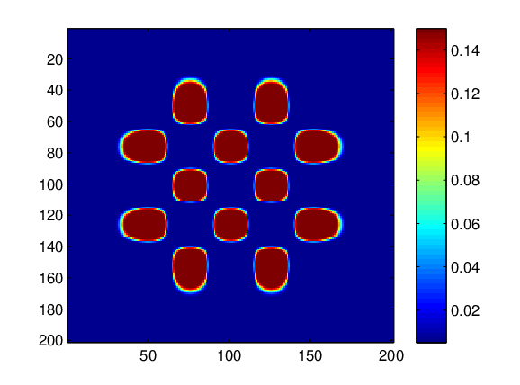
We solve the optimization problems using the TREGS [14] algorithm. We stop the optimization when the residual norm falls below 1.1 times the noise level. We report and compare the results for two cases in each experiment. First, we report results assuming that the full order problem was used to compute the function and Jacobian evaluation at each step. Then we report results using the ROM to replace the function and Jacobian evaluation. Figure 2 gives the absorption image using the initial set of parameters. We used systems for each experiment to create the reduced order model space. The tolerance in line 11 of Algorithm 1 was set to be . All of the experiments were run using a laptop with a GHz processor and GB RAM using MATLAB R2014a.
6.1 Experiment 1
In Experiment , we needed to solve large, single right-hand side systems to generate what we needed to construct the global basis matrix (note that the 64 of these corresponding to could have been pre-computed off-line). Including the additional eigenvectors of that were used as the first 10 columns of , has 197 columns and thus the reduced model has order . Therefore, the reduced models require solutions to linear systems of size rather than for the full order model.
The optimization using the full order model for Experiment required function evaluations and Jacobian evaluations. In comparison, the optimization run using the reduced order model, once it’s been generated, for function and Jacobian evaluations required function evaluations and Jacobian evaluations, indicating that using a ROM in place of FOM does not greatly impact convergence rate of the optimization. The bottom line is that solving the optimization using the full order model requires the solution of 1440 systems of size . On the other hand, solving using our approach requires solution of 187 systems of size , which are used to construct during the first few optimization steps. The remainder of the work is in solving systems of size until the convergence tolerance for the optimization is achieved.
Figure 3 shows the reconstructions for Experiment . Figure 1 also includes the number of (unpreconditioned) MINRES iterations for each experiment with and without recycling. Although the tables only show a sample of results, it is clear that the iterations decrease from one right-hand side to the next, and system to system, using our approach. The jump in number of iterations for right-hand-side comes from the fact that we concatenated and to form one right-hand-side for the symmetric transfer function, so the 33rd right-hand side corresponds to the first column in .


| Experiment 1 | Experiment 2 | ||||
| System | RHS | MINRES Its | MINRES Its | MINRES Its | MINRES Its |
| with Recycling | with Recycling | ||||
| 1 | 1 | 463 | 140 | 470 | 127 |
| 20 | 541 | 52 | 506 | 53 | |
| 32 | 487 | 0 | 493 | 0 | |
| 33 | 467 | 124 | 470 | 120 | |
| 53 | 528 | 57 | 514 | 48 | |
| 64 | 489 | 0 | 494 | 0 | |
| 2 | 1 | 474 | 118 | 501 | 124 |
| 20 | 513 | 35 | 545 | 38 | |
| 32 | 497 | 0 | 526 | 5 | |
| 33 | 474 | 105 | 500 | 132 | |
| 53 | 526 | 37 | 567 | 127 | |
| 64 | 497 | 0 | 532 | 0 | |
6.2 Experiment 2
In Experiment , a total , 40401 x 40401 single-right-hand side systems were solved to compute our global basis. The reduced order model has order . Therefore, the reduced models require solutions to linear systems of size rather than for the full order model. The optimization using the full order model required function evaluations and Jacobian evaluations. The optimization run using our reduced order model took function evaluations and Jacobian evaluations to converge to our stopping criterion, so again, there is no negative impact on convergence rate by replacing the FOM with the ROM. The difference in the total number of large (40401 x 40401) single-right-hand side systems that need to be solved, though, is even more pronounced in this example than in the last: 6,528 are needed for the FOM approach vs. only 188 for the ROM approach. Moreover, the work involved in solving for the latter systems is reduced, since MINRES requires fewer iterations due to the recycling.
Figure 4 shows the reconstructions for Experiment . Again, Figure 1 shows the number of unpreconditioned MINRES iterations for each experiment with and without our inner-outer recycling approach.


6.3 Value of Inner-Outer Recycling
There is a significant benefit to using two levels of recycling information. To see this, consider Algorithm 1 to construct the global basis. We could solve the full order model systems in Step 1 (e.g. systems in 25) with the unpreconditioned MINRES recycling approach in [21]. It is important to note that the recycle spaces would be different than those used in our new method. Furthermore, in the new method we solve the correction equations (44) as opposed to solving (25). For , the recycle spaces for the [21] approach do not incorporate information from other systems corresponding to other right-hand sides. In contrast, since we augment from information about right-hand side , we update . The update in then causes updates to , which are the right-hand sides in (44).
Table 2 compares the recycling of [21] with our new approach. The results show that with our approach, the number of iterations and the relative residuals decrease as you move from one right-hand-side to the next and also as you move from system to system. The jump at right-hand-side is due to the fact that you are moving to the second half of the concatenated right-hand-sides, so these correspond to solving the adjoint problem. Using the approach in [21], however, does not speed up convergence across right-hand-sides. In our approach, the reduced global basis, , is already constructed when we are done with the full order model solves. We note there is a big difference in total number of MINRES iterations to squeeze all information from systems and . It took our approach iterations, while it took iterations for the recycling method in [21].
| Our Approach | Recycling from [21] | ||||
|---|---|---|---|---|---|
| System | RHS | Its | Initial Relative Residual | Its | Initial Relative Residual |
| 1 | 1 | 140 | 7.523115e-05 | 140 | 7.523329e-05 |
| 20 | 52 | 1.077645e-06 | 185 | 6.584893e-04 | |
| 32 | 0 | 8.866398e-08 | 152 | 1.164802e-04 | |
| 33 | 124 | 4.776975e-05 | 127 | 5.213653e-05 | |
| 53 | 57 | 1.692149e-06 | 191 | 6.114295e-04 | |
| 64 | 0 | 9.960690e-08 | 151 | 1.450962e-04 | |
| 2 | 1 | 118 | 4.673235e-05 | 131 | 5.091877e-05 |
| 20 | 35 | 6.653493e-07 | 190 | 6.171251e-04 | |
| 32 | 0 | 8.754708e-08 | 153 | 1.051619e-04 | |
| 33 | 105 | 2.588292e-05 | 129 | 3.388392e-05 | |
| 53 | 37 | 8.454303e-07 | 188 | 6.405050e-04 | |
| 64 | 0 | 7.960101e-08 | 151 | 9.958796e-05 | |
7 Conclusions and Future Work
First, we established that our transfer function at zero frequency for DOT could be re-written in terms of a SPD matrix. Then, we developed an inner-outer Krylov recycling approach to update the global basis matrix relative to our new formulation of the transfer function. Two numerical experiments illustrate the success in using the ROM in place of the FOM during the optimization.
In this paper, we only considered the frequency case. It is non-trivial to extend the algorithm to the case when is non-zero, and it is therefore the subject of a forthcoming paper.
Clearly, the performance of our method depends on the values of some parameters, such as the residual tolerance and the number of systems . We found, for example, that if we dropped the tolerance slightly, the number of system solves, and therefore the reduced model order, was even further reduced, without too much degradation in the reconstruction. Likewise, using a larger value of gave slightly larger reduced order models, but with no improvement in the quality of the reconstruction. The trade-offs in performance due to these selections are currently under investigation. Finally, preliminary results indicate that solving the systems corresponding to different right-hand sides in a different ordering may also have an impact on the model order, and we will continue to investigate this phenomenon.
References
- [1] A. Aghasi, E. Miller, and M. E. Kilmer. Parametric level set methods for inverse problems. SIAM Journal on Imaging Science, 4:618–650, 2011.
- [2] K. Ahuja, E. de Sturler, and P. Benner. Recycling bicgstab with an applicaiton to parametric model order reduction. SIAM J. Sci. Comput., 37:S429–S446, 2015.
- [3] H. Antil, M. Heinkenschloss, and R. H. W. Hoppe. Domain decomposition and balanced truncation model reduction for shape optimization of the Stokes system. Optimization Methods and Software, 26(4–5):643–669, 2011.
- [4] H. Antil, M. Heinkenschloss, R. H. W. Hoppe, C. Linsenmann, and A. Wixforth. Reduced order modeling based shape optimization of surface acoustic wave driven microfluidic biochips. Mathematics and Computers in Simulation, 82(10):1986–2003, 2012.
- [5] E. Arian, M. Fahl, and E. Sachs. Trust-region proper orthogonal decomposition models by optimization methods. In Proceedings of the 41st IEEE Conference on Decision and Control, pages 3300–3305, Las Vegas, NV, 2002. IEEE.
- [6] S. R. Arridge. Optical tomography in medical imaging. Inverse Problems, Vol. 16:R41–R93, 1999.
- [7] O. Bashir, K. Willcox, O. Ghattas, B. van Bloemen Waanders, and J. Hill. Hessian-based model reduction for large-scale systems with initial condition inputs. International Journal for Numerical Methods in Engineering, 73(6):844–868, 2008.
- [8] U. Baur, C. Beattie, P. Benner, and S. Gugercin. Interpolatory projection methods for parameterized model reduction. SIAM Journal on Scientific Computing, 33:2489–2518, 2011.
- [9] C. Beattie, S. Gugercin, and S. Wyatt. Inexact solves in interpolatory model reduction. Linear Algebra and its Applications, 2011. Appeared on-line as doi:10.1016/j.laa.2011.07.015.
- [10] P. Benner, S. Gugercin, and K. Willcox. A survey of projection-based model reduction methods for parametric dynamical systems. SIAM Review, 57(4):483–531, 2015.
- [11] L. Borcea, V. Druskin, A. V. Mamonov, and M. Zaslavsky. A model reduction approach to numerical inversion for a parabolic partial differential equation. arXiv preprint arXiv:1210.1257, 2012.
- [12] E. de Sturler. Nested Krylov methods based on GCR. J. Comput. Appl. Math., 67(1):15–41, 1996.
- [13] E. de Sturler, S. Gugercin, M. E. Kilmer, S. Chaturantabut, C. Beattie, and M. O’Connell. Nonlinear parametric inversion using interpolatory model reduction. SIAM J. Sci. Comput., 37, 2015.
- [14] E. de Sturler and M. E. Kilmer. A regularized Gauss-Newton trust region approach to imaging in diffuse optical tomography. SIAM Journal on Scientific Computing, 33:3057 – 3086, 2011.
- [15] V. Druskin, V. Simoncini, and M. Zaslavsky. Solution of the time-domain inverse resistivity problem in the model reduction framework Part I. One-dimensional problem with SISO data. SIAM Journal on Scientific Computing, 35(3):A1621–A1640, 2013.
- [16] L. Feng, P. Benner, and J. G. Korvink. Parametric model order reduction accelerated by subspace recycling. In Proceedings of the 48th IEEE Conference on Decision and Control. IEEE, IEEE, 2009.
- [17] L. Feng, P. Benner, and J. G. Korvink. Subspace recycling accelerates the parametric macromodeling of MEMS. Int. J. Numer. Methods Eng., 94:84–110, 2013.
- [18] S. Gugercin, T. Stykel, and S. Wyatt. Model reduction of descriptor systems by interpolatory projection methods. SIAM Journal on Scientific Computing, 35(5):B1010–B1033, 2013.
- [19] E. Haber, U. M. Ascher, and D. Oldenburg. On optimization techniques for solving nonlinear inverse problems. Inverse Problems, 16:1263–1280, 2000.
- [20] M. Hinze and S. Volkwein. Proper orthogonal decomposition surrogate models for nonlinear dynamical systems: Error estimates and suboptimal control. In Dimension Reduction of Large-Scale Systems, pages 261–306. Springer, 2005.
- [21] M. Kilmer and E. de Sturler. Recycling subspace information for diffuse optical tomography. SIAM Journal on Scientific Computing, 27(6):2140–2166, 2006.
- [22] K. Kunisch and S. Volkwein. Proper orthogonal decomposition for optimality systems. ESAIM: Mathematical Modelling and Numerical Analysis, 42(1):1–23, 1 2008.
- [23] L. A. M. Mello, E. de Sturler, G. H. Paulino, and E. C. N. Silva. Recycling Krylov subspaces for efficient large-scale electrical impedance tomography. Computer Methods in Applied Mechanics and Engineering, 199:3101–3110, 2010.
- [24] A. Stathopoulos, A. M. Abdel-Rehim, and K. Orginos. Deflation for inversion with multiple right-hand sides in QCD. Journal of Physics: Conference Series 180, 2009.
- [25] A. Stathopoulos, A. M. Abdel-Rehim, and W. Wilcox. Deflated bicgstab for linear equations in QCD. pages 026/1–026/7, 2007. Proceedings of Science LAT2007.
- [26] C. R. Vogel. Computational Methods for Inverse Problems. SIAM, Philadelphia, 2002.
- [27] S. Wang, E. de Sturler, and G. Paulino. Large-scale topology optimization using preconditioned Krylov subspace methods with recycling. International Journal for Numerical Methods in Engineering, 69:2441–2461, 2007.
- [28] Y. Yue and K. Meerbergen. Accelerating optimization of parametric linear systems by model order reduction. SIAM Journal on Optimization, 23(2):1344–1370, 2013.