Economics; econophysics, financial markets, business and management Interdisciplinary applications of physics Networks and genealogical trees
Market correlation structure changes around the Great Crash
Abstract
We perform a comparative analysis of the Chinese stock market around the occurrence of the 2008 crisis based on the random matrix analysis of high-frequency stock returns of 1228 stocks listed on the Shanghai and Shenzhen stock exchanges. Both raw correlation matrix and partial correlation matrix with respect to the market index in two time periods of one year are investigated. We find that the Chinese stocks have stronger average correlation and partial correlation in 2008 than in 2007 and the average partial correlation is significantly weaker than the average correlation in each period. Accordingly, the largest eigenvalue of the correlation matrix is remarkably greater than that of the partial correlation matrix in each period. Moreover, each largest eigenvalue and its eigenvector reflect an evident market effect, while other deviating eigenvalues do not. We find no evidence that deviating eigenvalues contain industrial sectorial information. Surprisingly, the eigenvectors of the second largest eigenvalues in 2007 and of the third largest eigenvalues in 2008 are able to distinguish the stocks from the two exchanges. We also find that the component magnitudes of the some largest eigenvectors are proportional to the stocks’ capitalizations.
pacs
89.65.Ghpacs
89.20.-apacs
89.75.Hc1 Introduction
Financial markets evolve in a self-organized manner with the interacting elements forming complex networks at different levels, including international markets [1, 2, 3, 4], individual markets [5, 6, 7, 8], and security trading networks [9, 10, 11, 12, 13, 14, 15, 16]. There are well-documented stylized facts of stock return time series within individual markets unveiled by the random matrix theory (RMT) analysis [6, 17]: (1) The largest eigenvalue reflects the market effect such that its eigenportfolio returns are strongly correlated with the market returns; (2) Other largest eigenvalues contain information of industrial sectors; and (3) The smallest eigenvalues embed stock pairs with large correlations. However, for stock exchange index returns [1] and housing markets [18, 19], the largest eigenvalues can be used to extract geographic traits. Moreover, the signs of eigenvector components contain information of local interactions [20, 21, 18].
Financial crises occur more frequently than people usually expect, during which financial markets experience abrupt regime changes like phase transitions [22, 23]. The market correlation structure changes around financial crashes. The average correlation after the critical point of crash is higher than that before the crash [17, 3, 24]. Also, the correlation network becomes more connected after the crash [25]. It is natural that the absorption ratio of the largest eigenvalue serves as a measure of systemic risk [26].
On the other hand, the partial correlation analysis, which is a powerful tools for investigating the intrinsic correlation between two time series effected by common factors [27], has been applied to financial markets [17, 28, 29, 18, 30, 31, 32, 19]. An intriguing feature is that the partial correlation analysis is able to identify influences among different time series [30].
Applying the random matrix theory analysis to the 1-min high-frequency returns of Chinese stocks, we investigate in this work the correlation structure changes around the breakout of the Great Crash at the end of 2007 [33]. We focus on unveiling the information contents embedded in the deviating eigenvalues and their associated eigenvectors of the raw and partial correlation matrices. Novel results are found.
2 Data sets
We investigate the 1-min return time series of 489 A-share stocks traded on the Shenzhen Stock Exchange (SZSE) and 739 A-share stocks traded on the Shanghai Stock Exchange (SHSE) in 2007 and 2008, totally 1228 stocks, which were kindly provided by RESSET (http://resset.cn/). These stocks are chosen such that they have been listed before 2007 and had at least 180 trading days in each year.
The SZSE stocks belong to 16 industrial sectors including manufacturing (C, 306, 62.58%), real estate (K, 39, 7.98%), wholesale and retail industry (F, 39, 7.98%), electric power, heat, gas and water production and supply (D, 26, 5.32%), transport, storage and postal service (G, 14, 2.86%), mining (B, 11, 2.25%), information transmission, software and information technology services (I, 10, 2.04%), and 9 other industries. The SHSE stocks belong to 18 industrial sectors including manufacturing (C, 397, 53.72%), wholesale and retail industry (F, 74, 10.01%), real estate (K, 54, 7.31%), transport, storage and postal service (G, 47, 6.36%), electric power, heat, gas and water production and supply (D, 41, 5.55%), mining (B, 23, 3.11%), information transmission, software and information technology services (I, 21, 2.84%), and 11 other industries.
The 1-min logarithmic returns of stock are calculated as follows
| (1) |
where denotes the price of stock at time and . The returns are calculated at the intraday manner and no overnight returns are considered.
3 Distributions of correlation coefficients and partial correlation coefficients
For each year, 2007 or 2008, we calculate the correlation coefficient between the returns of stock and stock , which form the correlation matrix , as follows:
| (2) |
where and are the standard deviations of and . It is common that the 1-min trading time sequences of stock and stock do not overlap. Under such circumstance, we discard those times appeared in only one stock. For two arbitrary return time series and , we can extract their idiosyncratic components by removing a common collective component and calibrating the following simple univariate factor model:
| (3) |
where is the 1-min return time series of the Shanghai Stock Exchange Composite Index (SSCI). The partial correlation coefficient between and with respect to is defined as the correlation coefficient between the two residuals and :
| (4) |
where and are the standard deviations of and . We denote the partial correlation matrix. Simple algebraic manipulations result in the following equation [27, 29]
| (5) |
where () is the correlation coefficient between () and .

Fig. 1 illustrates that the distributions and of correlation coefficients and partial correlation coefficients in 2007 and 2008. The overwhelming majority of are positive and the distributions are rightly skewed. The average correlation coefficient in 2007 () is slightly smaller than that in 2008 (), implying that the Chinese stock market was in high risk and this systemic risk is higher in the panic bearish period than in the mania bullish period. The average correlation coefficients of 1-min returns are significantly smaller than those of daily returns (about 0.35) [34, 24], which is due to the fact that high-frequency returns are more noisy. The maximum correlation coefficient is 0.314 in 2007 and 0.386 in 2008.
After removing the influence of SSCI, the distributions and become narrower with the average partial correlation coefficients closer to 0 when compared with and , the bulk parts with of the two distributions almost overlap, and the discrepancy between the two distributions and becomes much smaller. It suggests that the discrepancy between and is mainly caused by a market effect. We further observe that there are more negative partial correlation coefficients in 2007 and more positive partial correlation coefficients in 2008. However, the proportions are low.
4 Distributions of eigenvalues
For the correlation matrix and the partial correlation matrix, we can determine their eigenvalues and the associated eigenvectors. When the observed time series have zero mean and unit variance, in the limit , where is fixed, the random matrix theory predicts that the distribution of eigenvalues can be expressed as [35, 36]
| (6) |
for , where and are respectively given by
| (7) |
which predicts a finite range of eigenvalues determined by the ratio .
There are stocks in our sample. For the raw and partial correlation matrices in 2007, and thus . We obtain that and . For the raw and partial correlation matrices in 2008, and thus . We obtain that and . These characteristic values are summarized in Table 1. Note that the results are essentially the same if we construct the random matrix from shuffled return time series [37, 18].
| 0.728 | 1.315 | 130.8 | 27.04% | 3.75% | |
| 0.731 | 1.311 | 148.9 | 28.34% | 2.20% | |
| 0.728 | 1.315 | 41.89 | 15.39% | 7.00% | |
| 0.731 | 1.311 | 41.90 | 14.01% | 5.94% |
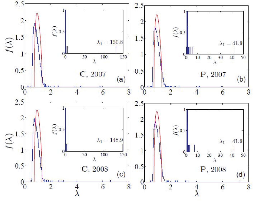
To identify that the estimated cross-correlations between stock returns are not a result of randomness, we compare in Fig. 2 the empirical eigenvalue distributions of the raw and partial correlation matrices and with the RMT prediction given by Eq. (6). It is somewhat “trivial” to observe that all the empirical eigenvalue distributions deviate significantly from the RMT prediction.
For the raw correlation matrices , there are 46 eigenvalues (3.75%) exceeding in 2007 and 27 eigenvalues (2.20%) exceeding in 2008. However, the largest eigenvalue in 2008 is greater than in 2007. Since is a measure of systemic risk [26], we argue that the Chinese stock market has a higher systemic risk in 2008 than in 2007. Moreover, the largest eigenvalue captures 11.6% of the variations in the return time series in 2007 and 12.1% of the variations in 2008. We also find that 332 eigenvalues (27.04%) are less than in 2007 and 348 eigenvalues (28.34%) are less than in 2008. All these deviating eigenvalues and the associated eigenvectors might contain significant economic information.
For the partial correlation matrices , there are 86 eigenvalues (7.00%) exceeding in 2007 and 73 eigenvalues (5.94%) exceeding in 2008. Surprisingly, the largest eigenvalue in 2008 is almost equal to in 2007, indicating that the higher systemic risk in 2008 was mainly introduced by the co-movements of stocks. In addition, the largest eigenvalue accounts for about 3.4% of the variations in the return residual time series in 2007 and 2008. We also find that 189 eigenvalues (15.39%) are less than in 2007 and 172 eigenvalues (14.01%) are less than in 2008. Overall, after removing the influence of SSCI, the eigenvalue distribution becomes much closer to the RMT prediction.


5 Eigenvectors of the largest eigenvalues
We now turn to unveil the economic information embedded in the first few largest eigenvalues of each matrix. Fig. 3 shows the associated eigenvectors of the five largest eigenvalues of the raw and partial correlation matrices in 2007 and 2008. Strikingly, there are no significant differences between the two eigenvectors associated with the -th largest eigenvalue of the raw and partial correlation matrices in a given year. However, we observe significant differences for the eigenvectors in different years. We thus focus on the discussions of the raw correlation matrices below.
| 2007 | 2008 | |||||
|---|---|---|---|---|---|---|
| SZSE | 93.86% | 0 | 49.64% | 34.77% | ||
| SHSE | 6.14% | 100% | 50.36% | 65.23% | ||
| SZSE | 35% | 45% | 3.79% | 78.28% | ||
| SHSE | 65% | 55% | 96.21% | 21.72% | ||
The most intriguing pattern is observed in the eigenvector of the second largest eigenvalue in 2007 and in the eigenvector of the third largest eigenvalue in 2008. In the eigenvector of 2007, 93.86% of the positive components correspond to SZSE stocks and 6.14% to SHSE stocks, while all the negative components are associated with SHSE stocks, as shown in Table 2. In the eigenvector of 2008, 3.79% of the positive components correspond to SZSE stocks and 96.21% to SHSE stocks, while 78.28% of the negative components are associated with SZSE stocks. Therefore, the component signs of in 2007 and in 2008 are able to distinguish SZSE stocks from SHSE stocks. This feature is not clearly observed for other eigenvectors. For instance, in the eigenvector of 2008, half of the positive components come from SZSE stocks and 1/3 of the negative components from SZSE stocks.
6 Market effect
The deviating eigenvalues capture the collective behaviors of different groups of stocks and in particular the largest eigenvalue usually reflects the market effect [7]. The characteristic of a market effect is the eigenvector of the largest eigenvalue has roughly equal components on all of the stocks, showing a nice linear relationship between the returns of the eigenportfolio constructed from and of the market index [17]. Usually, other deviating eigenvalues do not reflect a market effect but the comovement of stocks in the same industrial sector [17], the same traits shared by stocks [34], or geographic localization [38]. However, it is also possible that other deviating eigenvalues also reflect a market effect, such as the USA housing market [18].
For each eigenvector associated with eigenvalue , we construct its eigenportfolio, whose returns are calculated by
| (8) |
where , and denotes the projection of the return time series on the eigenvector . The return time series of the SSCI, of the first eigenportfolio and of the second eigenportfolio of the partial correlation matrices are plotted in Fig. 4(a,c,e) for 2007 and in Fig. 4(b,d,f) for 2008. The results are almost the same for the raw correlation matrices, which is natural due to the similarity of corresponding eigenvectors of and shown in Fig. 3. It is found that is quite similar to in each year, while is very different from .

Fig. 4(g-j) present the scatter plots of market returns against the eigenportfolio returns () constructed from . We find that there is no linear dependence between and . No linear dependence is observed either for with (not shown in Fig. 4). In contrast, there is a nice linear dependence between and in each year. The slope is 0.815 in 2007 and 0.733 in 2008. For , the slope is in 2007 and in 2008. These observations suggest that the largest eigenvalue quantifies a common influence on all stocks, while the rest of deviating eigenvalues contain no information about such a market effect.
The results for the raw correlation matrices are well established for diverse stock markets, especially on the daily level [17, 34]. However, the results for the partial correlation matrices are somewhat surprising. It was expected that the largest eigenvalue is no longer associated with the market, since the effect of the index has been removed [28]. According to our results, this natural conjecture is surprisingly not true. On the contrary, similar phenomena were observed for daily stock returns [39].
7 Eigenvector components and stocks’ market capitalizations
We checked the components of eigenvectors associated with the smallest eigenvalues. There are a few components whose magnitudes are significantly greater than the averages. However, we did not observe solid evidence that the correlations of the corresponding return time series of these components are among the largest, which is different from the U.S. stock market [17] and the global crude oil market [38].


(a)
(b)
(c)
(d)
(e)
(f)
We investigated the relationship between the eigenvector components and stocks’ market capitalizations. Fig. 5 illustrates the results for , and of the raw correlation matrix. The results for the partial correlation matrices are similar, as elaborated by the eigenvectors in Fig. 3. The eigenvector components of are positively correlated with the corresponding capitalizations, as shown in Fig. 5(a) and (b). For other largest eigenvalues, such positive correlations between the component magnitudes and capitalizations are observed for positive components or negative components. These findings suggest that stocks with low volatility and high liquidity exhibit high magnitudes of the eigenvector components.
8 Conclusion
We have conducted a comparative analysis of the information contents embedded in the largest eigenvalues of the raw and partial correlation matrices constructed from the 1-min high-frequency returns of Chinese stocks in 2007 and 2008. We identified market correlation structure changes around the Great crash in several aspects. In addition, although the correlation coefficient distributions and the largest eigenvalues of the raw and partial correlation matrix are significantly different in each period, the eigenvectors of the raw and partial correlation matrices in each period are strikingly similar. We found that the largest eigenvalue of each matrix reflects the whole market mode. It is found that the eigenvectors of the second largest eigenvalues in 2007 and of the third largest eigenvalues in 2008 are able to distinguish the stocks from the two exchanges, which are different from the cases of the U.S.A. stock market [17] and the Chinese stock market when daily returns are analyzed [34, 24]. We also found that the component magnitudes of the some largest eigenvectors are proportional to the stocks’ capitalizations.
Acknowledgements.
This work was partly supported by the National Natural Science Foundation of China (71532009 and 71131007) and the Fundamental Research Funds for the Central Universities.References
- [1] \NameSong D.-M., Tumminello M., Zhou W.-X. Mantegna R. N. \REVIEWPhys. Rev. E 842011026108.
- [2] \NameKumar S. Deo N. \REVIEWPhys. Rev. E 862012026101.
- [3] \NameNobi A., Maeng S. E., Ha G. G. Lee J. W. \REVIEWJ. Korean Phys. Soc. 622013569.
- [4] \NameNobi A., Lee S. M., Kim D. H. Lee J. W. \REVIEWPhys. Lett. A 27820142482.
- [5] \NameMantegna R. N. \REVIEWEur. Phys. J. B 111999193.
- [6] \NamePlerou V., Gopikrishnan P., Rosenow B., Amaral L. A. N. Stanley H. E. \REVIEWPhys. Rev. Lett. 8319991471.
- [7] \NameLaloux L., Cizeau P., Bouchaud J.-P. Potters M. \REVIEWPhys. Rev. Lett. 8319991467.
- [8] \NameKwapień J. Drożdż S. \REVIEWPhys. Rep. 5152012115.
- [9] \NameJiang Z.-Q. Zhou W.-X. \REVIEWPhysica A 38920104929.
- [10] \NameWang J.-J., Zhou S.-G. Guan J.-H. \REVIEWPhysica A 3902011398.
- [11] \NameSun X.-Q., Cheng X.-Q., Shen H.-W. Wang Z.-Y. \REVIEWPhysica A 39020113427.
- [12] \NameSun X.-Q., Shen H.-W., Cheng X.-Q. Wang Z.-Y. \REVIEWPLoS One 72012e45598.
- [13] \NameWang J.-J., Zhou S.-G. Guan J.-H. \REVIEWNeurocomputing 92201244.
- [14] \NameJiang Z.-Q., Xie W.-J., Xiong X., Zhang W., Zhang Y.-J. Zhou W.-X. \REVIEWQuant. Finance Lett. 120131.
- [15] \NameSun X.-Q., Shen H.-W. Cheng X.-Q. \REVIEWSci. Rep. 420143711.
- [16] \NameLi M.-X., Jiang Z.-Q., Xie W.-J., Xiong X., Zhang W. Zhou W.-X. \REVIEWPhysica A 4192015575.
- [17] \NamePlerou V., Gopikrishnan P., Rosenow B., Amaral L. A. N., Guhr T. Stanley H. E. \REVIEWPhys. Rev. E 652002066126.
- [18] \NameMeng H., Xie W.-J., Jiang Z.-Q., Podobnik B., Zhou W.-X. Stanley H. E. \REVIEWSci. Rep. 420143566.
- [19] \NameMeng H., Xie W.-J. Zhou W.-X. \REVIEWInt. J. Mod. Phys. B 2920151550181.
- [20] \NameJiang X.-F. Zheng B. \REVIEWEPL (Europhys. Lett.) 97201248006.
- [21] \NameJiang X.-F., Chen T.-T. Zheng B. \REVIEWSci. Rep. 420145321.
- [22] \NameSornette D. \BookWhy Stock Markets Crash (Princeton University Press, Princeton) 2003.
- [23] \NameSornette D. \REVIEWPhys. Rep. 37820031.
- [24] \NameRen F. Zhou W.-X. \REVIEWPLoS ONE 92014e97711.
- [25] \NameNobi A., Maeng S. E., Ha G. G. Lee J. W. \REVIEWPhysica A 4072014135.
- [26] \NameBillio M., Getmansky M., Lo A. W. Pelizzon L. \REVIEWJ. Financ. Econ. 1042012535.
- [27] \NameBaba K., Shibata R. Sibuya M. \REVIEWAust. N. Z. J. Stat. 462004657.
- [28] \NameKenett D. Y., Shapira Y. Ben-Jacob E. \REVIEWJ. Prob. Stat. 20092009249370.
- [29] \NameKenett D. Y., Tumminello M., Madi A., Gur-Gershgoren G., Mantegna R. N. Ben-Jacob E. \REVIEWPLoS One 52010e15032.
- [30] \NameKenett D. Y., Huang X.-Q., Vodenska I., Havlin S. Stanley H. E. \REVIEWQuant. Finance 152015569.
- [31] \NameUechi L., Akutsu T., Stanley H. E., Marcus A. J. Kenett D. Y. \REVIEWPhysica A 4212015488.
- [32] \NameQian X.-Y., Liu Y.-M., Jiang Z.-Q., Podobnik B., Zhou W.-X. Stanley H. E. \REVIEWPhys. Rev. E 912015062816.
- [33] \NameJiang Z.-Q., Zhou W.-X., Sornette D., Woodard R., Bastiaensen K. Cauwels P. \REVIEWJ. Econ. Behav. Org. 742010149.
- [34] \NameShen J. Zheng B. \REVIEWEPL (Europhys. Lett.) 86200948005.
- [35] \NameEdelman A. \REVIEWSIAM. J. Matrix Anal. & Appl. 91988543.
- [36] \NameSengupta A. M. Mitra P. P. \REVIEWPhys. Rev. E 6019993389.
- [37] \NameZhou W.-X., Mu G.-H. Kertész J. \REVIEWNew J. Phys. 142012093025.
- [38] \NameDai Y.-H., Xie W.-J., Jiang Z.-Q., Jiang G. J. Zhou W.-X. \REVIEWEmpir. Econ. 2016in press.
- [39] \NameSong D.-M. \BookComplexity Researches in Financial Markets Ph.D. thesis East China University of Science and Technology Shanghai (June 2013).