Turbulent reconnection of magnetic bipoles in stratified turbulence
Abstract
We consider strongly stratified forced turbulence in a plane-parallel layer with helicity and corresponding large-scale dynamo action in the lower part and non-helical turbulence in the upper. The magnetic field is found to develop strongly concentrated bipolar structures near the surface. They form elongated bands with a sharp interface between opposite polarities. Unlike earlier experiments with imposed magnetic field, the inclusion of rotation does not strongly suppress the formation of these structures. We perform a systematic numerical study of this phenomenon by varying magnetic Reynolds number, scale separation ratio, and Coriolis number. We focus on the formation of a current sheet between bipolar regions where reconnection of oppositely oriented field lines occurs. We determine the reconnection rate by measuring either the inflow velocity in the vicinity of the current sheet or by measuring the electric field in the reconnection region. We demonstrate that for large Lundquist numbers, , the reconnection rate is nearly independent of in agreement with results of recent numerical simulations performed by other groups in simpler settings.
Keywords:
Magnetohydrodynamics - turbulence - Sun: sunspots - dynamo1 Introduction
The mechanism for the formation of sunspots and active regions is still not understood. One popular model assumes that the solar dynamo generates thin, strong magnetic flux tubes of near the tachocline (D’Silva & Choudhuri, 1993). Part of these tubes can become magnetically buoyant and rise to the surface creating sunspots and active regions (Parker, 1955; Choudhuri et al., 1995); see also Fan (2009) for a review. So far neither numerical (Guerrero & Käpylä, 2011) nor observational (Fan, 2009; Zhao et al., 2013; Getling et al., 2016) studies have confirmed this scenario. Furthermore, the flux tubes are expected to expand as they rise, hence their strength weakens and some sort of re-amplification mechanism must complement this model to match the observational properties of sunspots.
An alternative mechanism for the formation of active regions and sunspots is based on the negative effective (mean-field) magnetic pressure instability (NEMPI). Analytical studies (Kleeorin et al., 1989; Kleeorin et al., 1990; Kleeorin et al., 1993; Kleeorin et al., 1996; Kleeorin & Rogachevskii, 1994; Rogachevskii & Kleeorin, 2007) supported by direct numerical simulations (Brandenburg et al., 2012; Käpylä et al., 2012; Käpylä et al., 2016) have shown that in stratified turbulence in the presence of a background magnetic field the effective magnetic pressure (the sum of turbulent and non-turbulent contributions) can become negative. This effect can give rise to a large-scale instability (Rogachevskii & Kleeorin, 2007; Kemel et al., 2013), i.e., NEMPI, which can lead to the concentration of a weak background magnetic field. Once the field becomes strong enough – more than the local equipartition value – the effective magnetic pressure is no longer negative and NEMPI is not excited. Direct numerical simulations (DNS) of stratified turbulence have demonstrated that NEMPI can produce magnetic field concentrations (Brandenburg et al., 2010; Brandenburg et al., 2011; Kemel et al., 2013; Jabbari et al., 2014) from background magnetic fields that can be either perpendicular or parallel to the density gradient in both spherical and rectangular domains. In the latter case, spot-like structures near the surface (Brandenburg et al., 2013; Brandenburg et al., 2014) are obtained. A further generalization to a two-layer model (Warnecke et al., 2013; Warnecke et al., 2016) with non-helical forcing in the lower layer and no forcing in the upper has been successful in generating bipolar magnetic structures with intriguing dynamical behavior. Furthermore, mean-field simulations have shown that the concentration of a background magnetic field by NEMPI can operate even in the presence of dynamo action (Jabbari et al., 2013).
Nevertheless, there are two limitations to the aforementioned studies: (a) it is necessary to have a weak initial background magnetic field to excite NEMPI, and (b) the maximum strength of the magnetic field in the nonlinear stage of NEMPI can be at most three times larger than the local equipartition value. Mitra et al. (2014) and Jabbari et al. (2015) have circumvented these limitations respectively in their Cartesian and spherical models by using a two-layer arrangement of forced stratified turbulence in which the bottom layer is helically forced and the top layer is non-helically forced. In both of these cases, a large-scale dynamo develops in the bottom layer and provides a background magnetic field that is concentrated by stratified turbulence in the top layer to generate intense magnetic structures of strengths that can be close to five times the equipartition value. It is not clear that NEMPI is the relevant mechanism that gives rise to the magnetic structures observed by Mitra et al. (2014) or Jabbari et al. (2015). Although Mitra et al. (2014) have not measured the effective magnetic pressure, they did detect large-scale downflows at the location of the magnetic flux concentrations. Similar downflows have been found previously in forced turbulence with an imposed vertical field (Brandenburg et al., 2013; Brandenburg et al., 2014), where NEMPI was found to lead to magnetic spot formation. In the work of Jabbari et al. (2015), NEMPI could only be excited in those parts of the domain where the strength of the dynamo-generated field was sufficiently below the equipartition magnetic field. Nevertheless, also in that case formation of spots coincided with downflows.
The purpose of the present study is two-fold. On the one hand, using the model of Mitra et al. (2014), we perform a systematic numerical study of the formation and decay of bipolar regions by varying different parameters of the problem, in particular the magnetic Reynolds number and the scale separation ratio. Furthermore, we study the effects of rotation through the Coriolis term in the same model. As emphasized by Mitra et al. (2014) and Jabbari et al. (2015), the lifetime of the sharp interface between the bipolar regions is much longer than what one estimates from the effects of turbulent diffusion. This suggests that the sharp interface is constantly being maintained by converging flows, which lead to the formation of a current sheet between two polarities and the occurrence of turbulent reconnection.
Magnetic reconnection is a fundamental plasma process that is believed to play an important role in different astrophysical, geophysical, and laboratory plasma phenomena, e.g., solar flares, coronal mass ejections, coronal heating, magnetospheric substorms and tearing mode instabilities in magnetic confinement fusion devices (Priest, 2014; Zweibel & Yamada, 2009; Loureiro et al., 2013). A classical model of reconnection was suggested by Parker (1957) and Sweet (1958); see also their later works (Sweet, 1969; Parker, 1994). According to the Sweet-Parker model, the reconnection rate is proportional to the square root of the magnetic diffusivity of the plasma. This would imply that in the astrophysically relevant limit of very small magnetic diffusivity (or very large Lundquist number) the Sweet-Parker reconnection rate would go to zero. Hence, for reconnection to be relevant in the astrophysical context it is necessary to find models of fast reconnection in which the reconnection rate is independent of Lundquist number in the asymptotic limit of large Lundquist number. Recently, fast reconnection has been studied in DNS of turbulent magnetohydrodynamics (MHD) in both two and three dimensions (Loureiro et al., 2009; Kowal et al., 2009; Huang & Bhattacharjee, 2010; Loureiro et al., 2012; Beresnyak, 2013; Oishi et al., 2015), and at least two competing models: by Lazarian & Vishniac (1999); Eyink et al. (2011) and by Uzdensky et al. (2010); Loureiro et al. (2013) have been proposed, see, e.g., Lazarian et al. (2015) for a review. To investigate the role of magnetic reconnection in our model, we zoom in on the flow around the sharp interface, study the dynamics of the current sheet in this region and measure the reconnection rate to determine which regime of turbulent reconnection is relevant to our system.
2 The model
2.1 Basic equations
To perform DNS of an isothermally stratified layer, we solve the equations for the velocity , the magnetic vector potential , and the density and, in some cases, also in the presence of nonvanishing angular velocity ,
| (1) |
| (2) |
| (3) |
where the operator is the advective derivative, is the traceless rate of strain tensor (the commas denote partial differentiation), is the kinematic viscosity, is the isothermal sound speed, is the vacuum permeability, is the magnetic diffusivity, is the magnetic field, and is the current density.
We perform simulations in a cubic domain of size . This implies that the smallest wavenumber which fits into the box is 1 (). We apply the same boundary condition as Mitra et al. (2014), i.e., we use periodic boundary conditions in the and directions, stress-free perfect conductor boundary conditions at the bottom of the domain, () and stress-free vertical field conditions at the top ().
The stratification is isothermal with constant gravity given by , so the density scale height is . In all the cases considered below we have and . In this setup the density contrast across the domain is . Since we have adopted an isothermal equation of state, there is no possibility of convection. We apply random volume forcing to drive turbulence. It is defined by a function that is -correlated in time and monochromatic in space. It consists of random non-polarized waves whose direction and phase change randomly at each time step. To simulate the two-layer model of Mitra et al. (2014), we define the forcing profile such that we have helical forcing in the lower part of the domain () and non-helical forcing in the upper (). Here, is the position of the border between helical and non-helical forcing; in our model we choose . The helical forcing leads to the generation of a large-scale magnetic field in the lower layer due to dynamo action. The field then diffuses to the upper layer where the magnetic bipolar spots are expected to form. For more details regarding the forcing profile, see Mitra et al. (2014).
This setup is chosen to demonstrate the physical effects in isolation. In particular, the region of the dynamo generating large-scale weakly non-uniform magnetic field is separated from the region where the strongly non-uniform bipolar magnetic region is formed. This arrangement can also mimic a nonuniform spatial distribution of kinetic helicity and effect in the solar convective zone, e.g., the is larger in the deeper parts of the convective zone (Krivodubskii, 1984).
2.2 Parameters of the simulations
To solve Eqs. (1)–(3), we perform DNS with the Pencil Code11 1 https://github.com/pencil-code. It uses sixth-order explicit finite differences in space and a third-order accurate time-stepping method. We use a numerical resolution of mesh points in the , , and directions. We choose our units such that . Our simulations are characterized by the fluid Reynolds number, , and the magnetic Prandtl number, , so the magnetic Reynolds number is . Here, is the forcing wavenumber, which takes a value of in most of our simulations. We also study the case . In all runs we keep, and vary .
As the value of the turbulent velocity is set by the local strength of the forcing, which is uniform, the turbulent velocity is also statistically uniform over depth, and therefore we choose to define as the root-mean-square velocity based on a volume average in the statistically steady state. On the other hand, the density varies over several orders of magnitude as a function of depth and hence we define the mean density as a a horizontally and temporally averaged density at each depth. The magnetic field is expressed in units of the local equipartition value, . Time is measured in turbulent-diffusive times, , where is the estimated turbulent magnetic diffusivity.
Most of the parameters are similar to those of Mitra et al. (2014), but we vary and also consider cases with rotation. We also study the effect of the scale separation ratio, , by changing to investigate its effect on the formation and evolution of bipolar structures. Table 1 shows all runs with their parameters.
We characterize the reconnection of the bipolar magnetic structures by the Lundquist number, :
| (4) |
where is the Alfvén velocity, and is a typical length scale, which is here taken to be the length of the current sheet.
Run D 16 30 0.042 RM0 10 30 0.05 RM1 50 30 0.014 RM1zs 50 30 0.013 RM1k 50 5 0.024 RM2 130 30 0.005 RM3 260 30 0.002 RM4 300 30 0.001

3 Properties of the dynamo
The magnetic field in our model is the result of a large-scale dynamo. We recall that the forcing in the momentum equation is fully helical in the lower of the box and non-helical in the rest. We expect that the dynamo generates an exponentially growing magnetic field during the early phase when the field is weak. The dynamo-generated field has a periodic behavior with dynamo waves propagating in the domain, where the forcing is helical (). To study the dynamo properties, we plot the butterfly diagram in Fig. 1. The upper panel shows the butterfly diagram at and the middle panel presents the same plot for . The speed of upward motion increases as one moves toward the surface for both polarities. The nondimensional growth rate is given as , where , and its value decreases with increasing magnetic Reynolds number (see Table 1 and the lower panel of Fig. 2). The large-scale magnetic field expands upward into the region with non-helical forcing due to turbulent magnetic diffusion. In this region, density is lower, so the field strongly exceeds the equipartition value. Here the field evolution is highly nonlinear and driven by the dynamo wave from beneath.
To measure the period of the dynamo cycle, we plot in the lower panel of Fig. 1 the value of as a function of time for two different depths, (inside the helical region; blue curve) and (near the surface; black curve). In Run D the value of the period is about for . This is consistent with the result of Mitra et al. (2014), where a period of the dynamo wave of was determined.
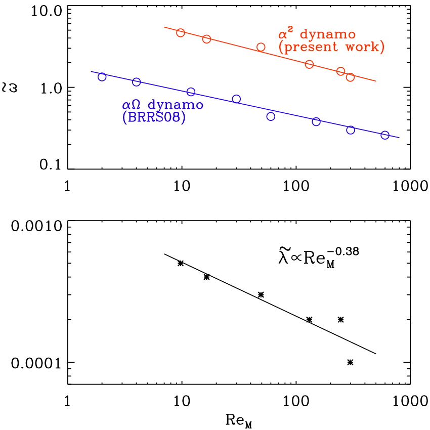
In the upper panel of Fig. 2 we show the dependence of the normalized dynamo frequency, , on the magnetic Reynolds number, . The fit overplotted on the data has the form
| (5) |
Although the large-scale dynamo that develops in this problem is an dynamo, the functional dependence of on is similar to that of a nonlinear dynamo in a Cartesian domain with linear shear (Käpylä & Brandenburg, 2009). In that case, is proportional to the quenched turbulent magnetic diffusivity, . In a separate study of a nonlinear dynamo, is found to be proportional to for (Brandenburg et al., 2008). The prefactor is, however, about 6 times larger in the present case of an dynamo compared to the earlier dynamos, where has been found; cf. Fig. 2. However, for much larger magnetic Reynolds numbers, as well as the growth rate of the large-scale dynamo instability might become independent of . Interestingly, the normalized growth of the dynamo displays a similar dependence on ; see the lower panel of Fig. 2. Specifically, we find .
The cyclic behavior of the dynamo-generated magnetic field is also shown in a series of snapshots in Fig. 3, where we present in the plane at different times. As one can see, dynamo waves propagate toward the surface and the evolution of the polarities is similar.

4 Magnetic structures
As mentioned above, the evolution and formation of the magnetic structures is similar to that of Mitra et al. (2014) and Jabbari et al. (2015). For 10, 16, and 50, bipolar magnetic structures of super-equipartition strength form in about half a turbulent-diffusive time and continue to evolve. For higher , structures form at later times and survive much longer compared to the case with a smaller of 10 or 16. However, the type of structures are otherwise similar for all .


4.1 Production of sharp fronts
In this paper we are interested in the time when structures develop and form “stripy” patterns at the surface (see Figs. 4 and 5). We concentrate on the phase in the evolution when different polarities move close together to form a current sheet between magnetic fields of the opposite polarities. Figure 5 illustrates the time evolution of at the surface (). One can see the formation of a sharp boundary between two polarities in the right column, third panel of this figure (). It is clear from Fig. 5 that the characteristic time of the formation of the elongated structures is of the order of the period of the dynamo wave, i.e., the turbulent-diffusion time (compare this figure with Fig. 3 for instance).
4.2 Relation to downflows
As follows from previous related studies of forced turbulence (Mitra et al., 2014), the magnetic flux concentrations tend to form in regions with downflows. To study this effect we plot in the upper panel of Fig. 7 the large-scale horizontal velocity, (blue arrows), together with a gray-scale representation of at the surface for . Here, denotes Fourier filtering, applied to obtain smoother contours. We see that there are positions where the horizontal velocity around or near the edge of the each spot is high. Furthermore, the horizontal velocity is small where the field is strong, which is consistent with the presence of downflows. This is shown in the lower panel of Fig. 7, where we plot in an plane through . There are indeed clear downflows below the magnetic flux concentration. This is in agreement with previous studies of magnetic field concentrations in one-layer turbulence.


4.3 Scale separation
Previous studies of magnetic flux concentrations in turbulence with weak imposed magnetic field have shown that NEMPI forms magnetic concentrations only when the scale separation ratio, , is about 15 or larger (Brandenburg et al., 2014). Therefore, we perform a simulation with to study whether the formation of structures is still possible in such a model. Figure 8 presents the visualization of at the surface of the box for such a simulation. Surprisingly, in our stratified two-layer forcing model, the bipolar magnetic structures continue to form, and follow a similar evolution as in the case with higher scale separation ratio. The only difference is the time delay in the formation of the first structure and their irregular and fast motions.
The other interesting case is when we apply a forcing profile that is helical in the entire domain (Run RM1zs). In such a system, we expect the formation of a bipolar structure at much earlier times, because the large-scale dynamo is now allowed to work in the entire domain so we should observe propagating dynamo waves at all depths. Our results confirm this already at a time of around , when a magnetic structure develops at the surface and the evolution of the structures occurs faster than in the two-layer simulations.
4.4 Evolution of bipolar structures
To investigate the evolution of the bipolar magnetic structures in more detail, we study the motion in the vicinity of the magnetic structures. In the early stage of the formation of bipolar structures, they tend to have round yin-yang shapes and each polarity rotates clockwise, independently of each other. When the structures move close enough to each other, their motion is no longer independent. After the formation of the elongated structures (see Fig. 5 at and ), one can see an anti-clockwise rotation at the border between opposite polarities (at and in this figure), which tends to break the connection and destroys the elongated structure. We suggest that the clockwise rotation of structures is due to the presence of a strong large-scale magnetic helicity associated with the structure. In other words, the traveling dynamo waves reach the surface and affect the evolution and motion of the magnetic structures. The anti-clockwise rotation, however, might be driven either by some instability, which occurs when opposite magnetic fields come close to each other (e.g., an instability similar to tearing instability during reconnection) or it might be caused by the interaction of two rotating polarities that are now coupled.


4.5 The effect of rotation
In this work we also study the effect of rotation on the formation and the evolution of the magnetic structures. We perform simulations with different Coriolis numbers, , , , and . Table 2 shows the parameters of these runs. Previous studies showed that for larger than 0.1, rotation suppresses the formation of magnetic structures by NEMPI, see Losada et al. (2013) and Jabbari et al. (2014). However, our present study shows that in our two-layer dynamo model, magnetic structures survive for as large as 1.4. It should also be noted that the combination of stratification and rotation leads to the generation of an additional contribution to the kinetic helicity in the system (Krause & Rädler, 1980; Kleeorin & Rogachevskii, 2003; Jabbari et al., 2014). This contribution is either constructive if (producing extra positive helicity) or destructive if (producing negative helicity). This could modify the dynamo action, but in the present case the Coriolis number is still too small for the rotation-induced helicity to be important; see Fig. 5 of Jabbari et al. (2014).
One of the possible reasons for the existence of magnetic structures for moderate rotation rates () is the large-scale dynamo that increases the magnetic flux. Indeed, NEMPI cannot create a new flux, but can only redistribute it by forming magnetic concentrations in certain small regions. Since the dynamo systematically produces new magnetic flux, and NEMPI redistributes it, the magnetic concentrations survive even for a moderate rotation.
Run RM1 0 0 0.0122 R1 0.037 0 0.041 R2 0.37 0 0.040 R3 0.74 0 0.033 R4 0.37 0.040 R5 0.37 0.040 R6 0 0.040 R7 1.4 0 0.015
It turns out that in the presence of rotation with , there is a delay in the formation of bipolar structures and the development of their shape during the early stage. In the case without rotation, the structure has spherical-like shape in the early stage of formation before it becomes elongated. This does not happen at finite rotation with . In the presence of rotation, even in the early stage of bipolar structure formation, it has a random elongated shape, which changes rapidly in time. In the presence of rotation it takes more time for the magnetic structures to become intense and concentrated.
5 Reconnection in the upper layers
The production of sharp fronts can be seen in Figs. 5 and 6, where we plot in two different planes. During the evolution of the magnetic structures, the bipolar regions evolve into stripes of opposite polarities separated by a current sheet; see Fig. 4. In Fig. 9 we zoom in on the sharp front in , where we also see vectors of and in the plane for our reference run. By comparing the field lines with Fig. 10, one can see a similar reconfiguration of magnetic field lines during spot evolution. It is clear from this figure that field lines with opposite signs of are reconnected and a component of the magnetic field is generated.


On a timescale that lies somewhere between the resistive diffusion and Alfvén timescales, magnetic reconnection occurs which causes the magnetic field topology to change and leads to the conversion of magnetic energy to thermal energy, kinetic energy and even particle acceleration; see the sketch in Fig. 10. According to Sweet-Parker theory (Parker, 1957; Sweet, 1958; Sweet, 1969; Parker, 1994), hereafter SP theory, the rate of reconnection, depends on the Lundquist number, :
| (6) |
In the turbulent regime of reconnection, is independent of the Ohmic resistivity (Lazarian & Vishniac, 1999); see also Eyink et al. (2011). This conclusion is supported by numerical simulations (Kowal et al., 2009). According to Lazarian & Vishniac (1999), the upper limit for the reconnection rate is:
| (7) |
where is the Alfvén Mach number.
For large Lundquist numbers, and in the turbulent regime of reconnection, is independent of . This conclusion is confirmed by recent numerical simulations (Loureiro et al., 2009; Huang & Bhattacharjee, 2010). For , the Sweet-Parker current sheet is unstable (Biskamp, 1986; Loureiro et al., 2005; Loureiro et al., 2012; Oishi et al., 2015). For spontaneous magnetic reconnection, according to magnetohydrodynamic numerical simulations (Loureiro et al., 2009; Huang & Bhattacharjee, 2010; Beresnyak, 2013), the rate of the reconnection, , for is of the order of
| (8) |
To determine , one can use two approaches. In one approach, the value of the inflow in the vicinity of the current sheet is measured (as sketched in Fig. 10). For a turbulent plasma, on the other hand, one can use a more general and accurate method. In this approach, one uses Ohm’s law:
| (9) |
so that the rate of the reconnection, , can be determined as , where
| (10) |
and angular brackets denote averaging along the direction (along the largest side of the current sheet, i.e., perpendicular to the current, see Fig. 10). Thus, the method of the determining in numerical simulations is as follows: (i) find the region with the current sheet that is separating magnetic fields of opposite polarities; (ii) use different instants of the formation of the current sheet and determine the value of , the length of the current layer, , in the direction, the Alfvén speed in these instants. Finally, we determine and , and compare these quantities with the obtained value of . We recall that the length of the current sheet enters in the definition , and the time when reaches its maximum value marks the starting time of reconnection.
To determine we use -averaged data, average over the interval , where is the length of the current sheet. Next, we measure the value of as and , while is a point, which is in the vicinity of the current sheet. Figure 10, upper panel, already shows the position of , which is the same for both and .
Run RM0 10 0.97 0.025 0.125 0.04 0.319 0.39 26 0.196 0.127 0.149 0.033 0.104 D1 16 0.65 0.0246 0.12 0.0136 0.231 0.52 28 0.188 0.0589 0.27 0.0101 0.0437 D1 16 0.84 0.0247 0.118 0.0206 0.299 0.4 37 0.165 0.0689 0.156 0.0212 0.0709 D1 16 0.97 0.123 0.104 0.0067 0.169 0.62 104 0.098 0.0397 0.379 0.0075 0.0444 RM1 50 2.87 0.0493 0.115 0.0107 0.228 0.5 187 0.073 0.047 0.254 0.0154 0.068 RM1 50 2.92 0.0493 0.120 0.0151 0.275 0.44 226 0.067 0.055 0.191 0.0211 0.077 RM1 50 2.99 0.0986 0.122 0.0099 0.323 0.38 531 0.043 0.031 0.143 0.0176 0.055 RM1 50 3.04 0.1478 0.126 0.0120 0.395 0.32 973 0.032 0.03 0.102 0.0184 0.047 RM1 50 3.09 0.1971 0.123 0.0108 0.441 0.28 1449 0.026 0.025 0.078 0.0145 0.033 RM1 50 3.16 0.1971 0.117 0.0071 0.435 0.27 1429 0.027 0.016 0.072 0.0093 0.022 RM1 50 3.21 0.5914 0.118 0.0121 0.395 0.3 3893 0.016 0.031 0.089 0.0137 0.035 RM1 50 3.34 1.7987 0.109 0.0061 0.322 0.34 9653 0.010 0.019 0.115 0.0112 0.035 RM1 50 3.46 1.3306 0.103 0.0060 0.239 0.43 5300 0.014 0.025 0.186 0.0092 0.039 RM1 50 3.58 0.9363 0.096 0.0075 0.176 0.55 2747 0.019 0.043 0.298 0.0104 0.059 RM1 50 3.71 0.4435 0.092 0.0053 0.130 0.71 961 0.032 0.041 0.501 0.0043 0.033 RM1 50 3.83 0.3450 0.094 0.0101 0.089 1.06 512 0.044 0.11 1.116 0.0107 0.12 RM2 130 1.6 2.4147 0.092 0.0039 0.183 0.50 22095 0.0067 0.0213 0.253 0.0058 0.032 RM2 130 1.65 1.7987 0.093 0.0089 0.181 0.51 16278 0.0078 0.0492 0.264 0.0094 0.052 RM2 130 1.7 1.4045 0.094 0.0074 0.187 0.50 13132 0.0087 0.0396 0.253 0.0091 0.049 RM2 130 1.75 1.1581 0.091 0.0080 0.194 0.47 11234 0.0094 0.0412 0.220 0.0094 0.049 RM2 130 1.8 0.8131 0.092 0.0080 0.187 0.49 7603 0.0115 0.0428 0.242 0.0094 0.050 RM2 130 1.9 0.5174 0.088 0.0051 0.151 0.58 3906 0.0160 0.0338 0.340 0.0074 0.049 RM3 260 3.04 0.468 0.09 0.005 0.198 0.455 9266 0.011 0.024 0.207 0.005 0.024 RM3 260 3.24 0.665 0.088 0.006 0.178 0.494 11837 0.009 0.033 0.245 0.005 0.028 RM3 260 3.33 2.538 0.086 0.004 0.165 0.521 41877 0.005 0.026 0.272 0.004 0.024 RM3 260 3.43 1.848 0.086 0.005 0.159 0.541 29383 0.006 0.032 0.293 0.003 0.021 RM3 260 3.53 1.010 0.086 0.006 0.154 0.558 15554 0.008 0.035 0.312 0.003 0.021 RM3 260 3.63 0.542 0.087 0.022 0.094 0.926 5094 0.014 0.233 0.857 0.007 0.070
The resulting values of are summarized in Table 3. For comparison, we measure both the velocity using Eq. (10) and the incoming velocity in the vicinity of the current sheet (in the case of a two-dimensional flow in the -plane it is in the direction). We normalize these velocities by , because varies with time (see Fig. 11). In this section, in order to be able to compare the results of different runs, we use for the normalized time, where is the time when the reconnection starts for each individual Run. Figure 11 presents the time evolution of the different quantities in three separate panels: and in the upper panel, and in the middle panel, and finally in the lower panel. The different colors represent different values of . One can see that, does not change strongly with time and changes when is smaller (). This implies that the major change in comes from the change in the length of the current sheet (see the lower panel of Fig. 11).

To check which regime of magnetic reconnection is appropriate, we plot in Fig. 12 as a function of . By comparing the curves for different magnetic Reynolds numbers, , , , it is clear that our data points are consistent with the turbulent regime of reconnection (Loureiro et al., 2009; Huang & Bhattacharjee, 2010; Loureiro et al., 2012; Beresnyak, 2013), where the reconnection rate is nearly independent of . Fig. 13 demonstrates that the reconnection rates obtained from the measurements of and are similar.


The dependence of the reconnection rate on is shown in Fig. 14. To compare the resulting data from our simulations with the model of Lazarian & Vishniac (1999), we also plot the linear fit to the data points in Fig. 14. It is clear that our data points strongly deviate from the predicted line, and are thus inconsistent with Lazarian & Vishniac (1999). However, is weakly dependent on the Ohmic resistivity (see Figs. 12 and 14), in agreement with Lazarian & Vishniac (1999).

6 Conclusions
In the present paper, we have extended the results of Mitra et al. (2014) to higher magnetic Reynolds numbers and have investigated the effects of rotation at different Coriolis numbers. Our results demonstrate that in the two-layer model with helical forcing in the lower part and non-helical forcing in the upper, sharp bipolar spots form at the surface, expand and then develop stripy structures. The observed effects are similar for different values of and . In our present simulations, for as large as 1.4, we still observe the formation of the intense bipolar structures. This value is significantly larger than what was previously obtained in studies of magnetic flux concentrations in rotating turbulence with an imposed weak magnetic field. One of the plausible explanations for this is the large-scale dynamo which increases magnetic flux. By contrast, NEMPI cannot produce new flux, but only redistribute it, forming magnetic concentrations in small regions. Thus, the large-scale dynamo systematically produces new magnetic flux, while NEMPI redistributes it. This could be the reason why the magnetic concentrations survive even for moderate rotation. Although there are dynamo-generated magnetic fields in our simulations, which is more realistic compared to several previous models with an imposed magnetic field, we still observe evidence for downflows at the locations of magnetic structure formation, similar to Brandenburg et al. (2014), Mitra et al. (2014), and Jabbari et al. (2015).
What is surprising is the long lifetime of the resulting bipolar regions, which exceeds several turbulent diffusion times. We suggest that the main reason why these intense magnetic structures survive longer is the magnetic reconnection phenomenon in the vicinity of the current sheet between opposite magnetic polarities. We have determined the reconnection rate for a range of different parameters and have shown that for high Lundquist numbers, , the measured reconnection rate is nearly independent of . This result is consistent with recent numerical simulations in a turbulent regime of reconnection performed by other groups (Loureiro et al., 2009; Huang & Bhattacharjee, 2010; Loureiro et al., 2012; Beresnyak, 2013). The measured reconnection rate is weakly dependent on the Alfvén Mach number, , which is inconsistent with predictions of Lazarian & Vishniac (1999). On the other hand, the reconnection rate is also weakly dependent on the Ohmic resistivity, in agreement with Lazarian & Vishniac (1999).
In the present work, we have also investigated the effects of varying the scale separation ratio, . Contrary to earlier studies of NEMPI, for as small as five, bipolar magnetic structures still form. Our previous studies of an unipolar magnetic concentrations with an imposed weak mean magnetic field have shown that, although the effective magnetic pressure (the sum of turbulent and non-turbulent contributions) becomes negative even for moderate scale separation ratio (about 3–5), the large-scale instability (NEMPI) is excited only if the scale separation ratio is large enough (). This suggests that the phenomenon we find in our DNS cannot be understood solely in terms of NEMPI.
In the more complicated two-layer system with a dynamo-generated magnetic field, two instabilities (dynamo and probably NEMPI or the magnetic buoyancy instability) may be excited. We stress that in both, our two-layer model with dynamo-generated magnetic field and in turbulent systems with an imposed magnetic field where NEMPI is known to be excited, strong density stratification plays an important role. Furthermore, there is evidence for the existence of downflows at the locations of magnetic structures in both systems. However, in our two-layer model the formation of bipolar regions is still observed for smaller scale separation ratios than what was required for a turbulent system with an imposed magnetic field where NEMPI was excited.
The process maintaining the bipolar structures may be related to or associated with NEMPI. It may also be possible that the positive magnetic pressure associated with the strong dynamo-generated magnetic field in nonlinear stage of evolution is responsible for the formation of the sharp interface of the bipolar structures found in the upper layers, where the plasma beta is no longer very large. However, a conclusive answer cannot be given at present. To arrive at a more definitive conclusion regarding the mechanism of bipolar structure formation, it would be desirable to measure the effective magnetic pressure tensors in our two-layer model and to study its parameter dependency in more detail. This requires the development of an adequate test-field method. This is a subject of a separate study.
Acknowledgements
We appreciate valuable advise by Alexander Schekochihin and Nuno Loureiro to study magnetic reconnection in our two-layer system. We also acknowledge valuable discussions with Andrey Beresnyak and Alexandre Lazarian as well as constructive remarks from the referee. This work was supported in part by the Swedish Research Council Grants No. 621-2011-5076 (AB,SJ), 2012-5797 (AB), and 638-2013-9243 (DM), as well as the Research Council of Norway under the FRINATEK grant 231444 (AB, NK, IR). We acknowledge the allocation of computing resources provided by the Swedish National Allocations Committee at the Center for Parallel Computers at the Royal Institute of Technology in Stockholm, the High Performance Computing Center North in Umeå, and the Nordic High Performance Computing Center in Reykjavik.
References
- Beresnyak (2013) Beresnyak, A. 2013, arXiv: 1301.7424.
- Biskamp (1986) Biskamp, D. 1986, Phys. Fluids, 29, 1520
- Brandenburg et al. (2014) Brandenburg, A., Gressel, O., Jabbari, S., Kleeorin, N., & Rogachevskii, I. 2014, A&A, 562, A53
- Brandenburg et al. (2011) Brandenburg, A., Kemel, K., Kleeorin, N., Mitra, D., Rogachevskii, I. 2011, ApJ, 740, L50
- Brandenburg et al. (2012) Brandenburg, A., Kemel, K., Kleeorin, N., Rogachevskii, I. 2012, ApJ, 749, 179
- Brandenburg et al. (2010) Brandenburg, A., Kleeorin, N., & Rogachevskii, I. 2010, Astron. Nachr., 331, 5
- Brandenburg et al. (2013) Brandenburg, A., Kleeorin, N., & Rogachevskii, I. 2013, ApJ, 776, L23
- Brandenburg et al. (2008) Brandenburg, A., Rädler, K.-H., Rheinhardt, M., & Subramanian, K. 2008, ApJ, 687, L49
- Choudhuri et al. (1995) Choudhuri, A. R., Schüssler, M., & Dikpati, M. 1995, A&A, 303, L29
- D’Silva & Choudhuri (1993) D’Silva, S., & Choudhuri, A. R. 1993, A&A, 272, 621
- Eyink et al. (2011) Eyink, G. L., Lazarian, A. & Vishniac E. T. 2011, ApJ, 743, 51
- Fan (2009) Fan, Y. 2009, Living Rev. Solar Phys., 6, 4
- Getling et al. (2016) Getling, A. V., Ishikawa, R., & Buchnev, A. A., 2016, Solar Phys., in press; DOI: 10.1007/s11207-015-0844-3, arXiv:1506.01848
- Guerrero & Käpylä (2011) Guerrero, G. & Käpylä, P. J. 2011, A&A, 533, A40
- Huang & Bhattacharjee (2010) Huang, Y.-M. & Bhattacharjee, A. 2010, Phys. Plasmas, 17, 062104
- Jabbari et al. (2013) Jabbari, S., Brandenburg, A., Kleeorin, N., Mitra, D., & Rogachevskii, I. 2013, A&A, 556, A106
- Jabbari et al. (2014) Jabbari, S., Brandenburg, A., Losada, I. R., Kleeorin, N., & Rogachevskii, I. 2014, A&A, 568, A112
- Jabbari et al. (2015) Jabbari, S., Brandenburg, A., Kleeorin, N., Mitra, D.,& Rogachevskii, I. 2015, ApJ, 805, 166
- Käpylä & Brandenburg (2009) Käpylä, P. J., & Brandenburg, A. 2009, ApJ, 699, 1059
- Käpylä et al. (2012) Käpylä, P. J., Brandenburg, A., Kleeorin, N., Mantere, M. J., & Rogachevskii, I. 2012, MNRAS, 422, 2465
- Käpylä et al. (2016) Käpylä, P. J., Brandenburg, A., Kleeorin, N., Käpylä, M. J., & Rogachevskii, I. 2016, A&A, in press, arXiv:1511.03718
- Kemel et al. (2013) Kemel, K., Brandenburg, A., Kleeorin, N., Mitra, D., & Rogachevskii, I. 2013, Solar Phys., 287, 293
- Kleeorin et al. (1993) Kleeorin, N., Mond, M., & Rogachevskii, I. 1993, Phys. Fluids B, 5, 4128
- Kleeorin et al. (1996) Kleeorin, N., Mond, M., & Rogachevskii, I. 1996, A&A, 307, 293
- Kleeorin & Rogachevskii (1994) Kleeorin, N., & Rogachevskii, I. 1994, Phys. Rev. E, 50, 2716
- Kleeorin & Rogachevskii (2003) Kleeorin, N., & Rogachevskii, I. 2003, Phys. Rev. E, 67, 026321
- Kleeorin et al. (1989) Kleeorin, N.I., Rogachevskii, I.V., & Ruzmaikin, A.A. 1989, Sov. Astron. Lett., 15, 274
- Kleeorin et al. (1990) Kleeorin, N. I., Rogachevskii, I. V., Ruzmaikin, A. A. 1990, Sov. Phys. JETP, 70, 878
- Kowal et al. (2009) Kowal, G., Lazarian, A., Vishniac E. T., & Otmianowska-Mazur, K. 2009, ApJ, 700, 63
- Krause & Rädler (1980) Krause F., Rädler K.-H., 1980, Mean-Field Magnetohydrodynamics and Dynamo Theory. Pergamon, Oxford
- Krivodubskii (1984) Krivodubskii, V. N. 1984, Sov. Astron., 28, 205
- Lazarian & Vishniac (1999) Lazarian, A. & Vishniac E. T. 1999, ApJ, 517, 700
- Lazarian et al. (2015) Lazarian, A., Eyink, G. L., Vishniac, E. T., & Kowal, G. 2015, arXiv:1502.01396
- Losada et al. (2013) Losada, I. R., Brandenburg, A., Kleeorin, N., & Rogachevskii, I. 2013, A&A, 556, A83
- Loureiro et al. (2005) Loureiro, N. F., Cowley, S. C., Dorland, W. D., Haines, M. G. Schekochihin, A. A. 2005, Phys. Rev. Lett., 95, 235003
- Loureiro et al. (2009) Loureiro, N. F., Uzdensky, D. A., Schekochihin, A. A., Cowley, S. C., Yousef, T. A. 2009, MNRAS, 399, L146
- Loureiro et al. (2012) Loureiro, N. F., Samtaney, R., Schekochihin, A. A. & Uzdensky, D. A. 2012, Phys. Plasmas, 19, 042303
- Loureiro et al. (2013) Loureiro, N. F., Schekochihin, A. A., & Uzdensky, D. A. 2013, Phys. Rev. E, 87, 013102
- Mitra et al. (2014) Mitra, D., Brandenburg, A., Kleeorin, N., & Rogachevskii, I. 2014, MNRAS, 445, 761
- Oishi et al. (2015) Oishi, J. S., Mac Low, M.-M., Collins, D. C., & Tamura, M. 2015, ApJ, 806, L12
- Parker (1955) Parker, E. N. 1955, ApJ, 121, 491
- Parker (1957) Parker, E. N. 1957, J. Geophys. Res., 62, 509
- Parker (1994) Parker, E. N., Spontaneous current sheets in magnetic fields: with applications to stellar x-rays (Oxford University Press, USA, 1994)
- Priest (2014) Priest, E., Magnetohydrodynamics of the Sun (Cambridge University Press, New York, 2014)
- Rogachevskii & Kleeorin (2007) Rogachevskii, I., & Kleeorin, N. 2007, Phys. Rev. E, 76, 056307
- Sweet (1958) Sweet, P. A., Proc. IAU Symp. no. 6., p. 123 (1958).
- Sweet (1969) Sweet, P. A. 1969, ARA&A, 7, 149
- Uzdensky et al. (2010) Uzdensky, D. A., Loureiro, N. F., Schekochihin, A. A. 2010, Phys. Rev. Lett., 105, 235002
- Warnecke et al. (2013) Warnecke, J., Losada, I. R., Brandenburg, A., Kleeorin, N., & Rogachevskii, I. 2013, ApJ, 777, L37
- Warnecke et al. (2016) Warnecke, J., Losada, I. R., Brandenburg, A., Kleeorin, N., & Rogachevskii, I. 2016, A&A, in press, arXiv:1502.03799
- Zhao et al. (2013) Zhao, J., Bogart, R. S., Kosovichev, A. G., Duvall, Jr., T. L., & Hartlep, T. 2013, ApJ, 774, L29
- Zweibel & Yamada (2009) Zweibel, E. G., & Yamada, M. 2009, ARA&A, 47, 291