Positivity-preserving discontinuous Galerkin methods with Lax-Wendroff time discretizations
Abstract
This work introduces a single-stage, single-step method for the compressible Euler equations that is provably positivity-preserving and can be applied on both Cartesian and unstructured meshes. This method is the first case of a single-stage, single-step method that is simultaneously high-order, positivity-preserving, and operates on unstructured meshes. Time-stepping is accomplished via the Lax-Wendroff approach, which is also sometimes called the Cauchy-Kovalevskaya procedure, where temporal derivatives in a Taylor series in time are exchanged for spatial derivatives. The Lax-Wendroff discontinuous Galerkin (LxW-DG) method developed in this work is formulated so that it looks like a forward Euler update but with a high-order time-extrapolated flux. In particular, the numerical flux used in this work is a linear combination of a low-order positivity-preserving contribution and a high-order component that can be damped to enforce positivity of the cell averages for the density and pressure for each time step. In addition to this flux limiter, a moment limiter is applied that forces positivity of the solution at finitely many quadrature points within each cell. The combination of the flux limiter and the moment limiter guarantees positivity of the cell averages from one time-step to the next. Finally, a simple shock capturing limiter that uses the same basic technology as the moment limiter is introduced in order to obtain non-oscillatory results. The resulting scheme can be extended to arbitrary order without increasing the size of the effective stencil. We present numerical results in one and two space dimensions that demonstrate the robustness of the proposed scheme.
1 Introduction
1.1 Governing equations
The purpose of this work is to develop a positivity-preserving version of the Lax-Wendroff discontinuous Galerkin method for the compressible Euler equations on unstructured meshes. The compressible Euler equations form a system of hyperbolic conservation law that can be written as follows:
| (1) |
The conserved variables are the mass density, , the momentum density, , and the energy density, ; the primitive variables are the mass density, , the fluid velocity, , and the pressure, . The energy is related to the primitive variables through the equation of state,
| (2) |
where the constant is the ratio of specific heats (aka, the gas constant).
The compressible Euler equations are an important mathematical model in the study of gases and plasma. Attempts at numerically solving the these equations has led to a plethora of important historical advances in the development of numerical analysis and scientific computing (see e.g., [22, 29, 15, 32, 28]).
1.2 Discontinuous Galerkin spatial discretization
The focus of this work is on high-order discontinuous Galerkin (DG) methods, which were originally developed for general hyperbolic conservation laws by Cockburn, Shu, et al. in series of papers [13, 12, 10, 14, 11]. The purpose of this section is to set the notation used throughout the paper and to briefly describe the DG spatial discretization.
Let be a polygonal domain with boundary . The domain is discretized via a finite set of non-overlapping elements, , such that . Let denote the set of polynomials from to with maximal polynomial degree . Let denote the broken finite element space on the mesh:
| (3) |
where is the mesh spacing. The above expression means that has components, each of which when restricted to some element is a polynomial of degree at most and no continuity is assumed across element edges (or faces in 3D).
The approximate solution on each element at time is of the form
| (4) |
where is the number of Legendre polynomials and are the Legendre polynomials defined on the reference element in terms of the reference coordinates . The Legendre polynomials are orthonormal with respect to the following inner product:
| (5) |
We note that independent of , , , and the type of element, the lowest order Legendre polynomial is always . This makes the first Legendre coefficient the cell average:
| (6) |
1.3 Time stepping
The most common approach for time-advancing DG spatial discretizations is via explicit Runge-Kutta time-stepping; the resulting combination of time and space discretization is often referred to as the “RK-DG” method [10]. The primary advantage for this choice of time stepping is that explicit RK methods are easy to implement, they can be constructed to be low-storage, and a subclass of these methods have the so-called strong stability preserving (SSP) property [23], which is important for defining a scheme that is provably positivity-preserving. However, there are no explicit Runge-Kutta methods that are SSP for orders greater than four [26, 36].
The main difficulty with Runge-Kutta methods is that they typically require many stages; and therefore, many communications are needed per time step. One direct consequence of the communication required at each RK stage is that is difficult to combine RK-DG with locally adaptive mesh refinement strategies that simultaneously refine in both space and time.
The key piece of technology required in locally adaptive DG schemes is local time-stepping (see e.g., Dumbser et al. [17]). Local time-stepping is easier to accomplish with a single-stage, single-step (Lax-Wendroff) method than with a multi-stage Runge-Kutta scheme. For these reasons there is interest from discontinuous Galerkin theorists and practitioners in developing single-step time-stepping techniques for DG (see e.g., [43, 34, 18, 19, 42, 16, 21, 20]), as well as hybrid multistage multiderivative alternatives [38].
In this work, we construct a numerical scheme that uses a Lax-Wendroff time discretization that is coupled with the discontinuous Galerkin spatial discretization. In subsequent discussions in this paper we demonstrate the advantages of switching to single-stage and single-stage time-stepping in regards to enforcing positivity on arbitrary meshes.
1.4 Positivity preservation
In simulations involving strong shocks, high-order schemes (i.e. more than first-order) for the compressible Euler equations generally create nonphysical undershoots (below zero) in the density and/or pressure. These undershoots typically cause catastrophic numerical instabilities due to a loss of hyperbolicity. Moreover, for many applications these positivity violations exist even when the equations are coupled with well-understood total variation diminishing (TVD) or total variation bounded (TVB) limiters. The chief goal of the limiting scheme developed in this work is to address positivity violations in density and pressure, and in particular, to accomplish this task with a high-order scheme.
In the DG literature, the most widely used strategy to maintain positivity was developed by Zhang and Shu in a series of influential papers [47, 48, 49]. The basic strategy of Zhang and Shu for a positivity-preserving RK-DG method can be summarized as follows:
- Step 0.
-
Write the current solution in the form
(7) where is yet-to-be-determined. represents the unlimited solution.
- Step 1.
-
Find the largest value of , where , such that satisfies the appropriate positivity conditions at some appropriately chosen quadrature points and limit the solution.
- Step 2.
-
Find the largest stable time-step that guarantees that with a forward Euler time that the cell average of the new solution remains positive.
- Step 3.
-
Rely on the fact that strong stability-preserving Runge-Kutta methods are convex combinations of forward Euler time steps; and therefore, the full method preserves the positivity of cell averages (under some slightly modified maximum allowable time-step).
For a Lax-Wendroff time discretization, numerical results indicate that the limiting found in Step 1 is insufficient to retain positivity of the solution, even for simple 1D advection. Therefore, the strategy we pursue in this work will still contain an equivalent Step 1; however, in place of Step 2 and Step 3 above, we will make use of a parameterized flux, sometimes also called a flux corrected transport (FCT) scheme, to maintain positive cell averages after taking a single time step. In doing so, we avoid introducing additional time step restrictions that often appear (e.g., in Step 2. above) when constructing a positivity-preserving scheme based on Runge-Kutta time stepping.
This idea of computing modified fluxes by combining a stable low-order flux with a less robust high-order flux is relatively old, and perhaps originates with Harten and Zwas and their self adjusting hybrid scheme [25]. The basic idea is the foundation of the related flux corrected transport (FCT) schemes of Boris, Book and collaborators [4, 3, 5, 2], where fluxes are adjusted in order to guarantee that average values of the unknown are constrained to lie within locally defined upper and lower bounds. This family of methods is used in an extensive variety of applications, ranging from seismology to meteorology [46, 27, 50, 44]. A thorough analysis of some of the early methods is conducted in [41]. Identical to modern maximum principle preserving (MPP) schemes, FCT can be formulated as a global optimization problem where a “worst case” scenario assumed in order to decouple the previously coupled degrees of freedom [1]. Here we do not attempt to use FCT to enforce any sort of local bounds (in the sense of developing a shock-capturing limiter), instead we leverage these techniques in order to retain positivity of the density and pressure associated to ; such approaches have recently received renewed interest in the context of weighted essentially non-oscillatory (WENO) methods [45, 30, 9, 8, 39, 6].
To summarize, our limiting scheme draws on ideas from the two aforementioned families of techniques that are well established in the literature. First, we start with the now well known (high-order) pointwise limiting developed for discontinuous Galerkin methods [47, 48, 49], and second, we couple this with the very large family of flux limiters [8, 39, 6]. (developed primarily for finite-difference (FD) and finite-volume (FV) schemes).
1.5 An outline of the proposed positivity-preserving method
The compressible Euler equations (1) can be written compactly as
| (8) |
where the conserved variables are and the flux function is
| (9) |
where and .
The basic positivity limiting strategy proposed in this work is summarized below. Some important details are omitted here, but we elaborate on these details in subsequent sections.
- Step 0.
-
On each element we write the solution as
(10) where is yet-to-be-determined. represents the unlimited solution.
- Step 1.
-
Assume that this solution is positive in the mean. That is, we assume for all that and
(11) A consequence of these assumptions is that .
- Step 2.
-
Find the largest value of , where , such that the density and pressure are positive at some suitably defined quadrature points. This step is elaborated upon in §3.2.
- Step 3.
-
Construct time-averaged fluxes through the Lax-Wendroff procedure. That is, we start with the exact definition of the time-average flux:
(12) and approximate this via a Taylor series expansion around :
(13) All time derivatives in this expression are replaced by spatial derivatives using the chain rule and the governing PDE (8). The approximate time-averaged flux (13) is first evaluated at some appropriately chosen set of quadrature points – in fact, the same quadrature points as used in Step 2 – and then, using appropriate quadrature weights, summed together to define a high-order flux, at both interior and boundary quadrature points. Thanks to Step 2, all quantities of interest used to construct this expansion are positive at each quadrature point.
- Step 4.
-
Time step the solution so that cell averages are guaranteed to be positive. That is, we update the cell averages via a formula of the form
(14) where is an outward-pointing (relative to ) normal vector to edge with the property that is the length of edge , and the numerical flux on edge, , is a convex combination of a high-order flux, , and a low-order flux :
(15) The low-order flux, , is based on the (approximate) solution to the Riemann problem defined by cell averages only, and the “high-order” flux, , is constructed after integrating via Gaussian quadrature the (approximate) Riemann solutions at quadrature points along the edge :
(16) where are the Gaussian quadrature weights for quadrature with points and are the numerical fluxes at each of the quadrature points. Note that this sum has only a single summand in the one-dimensional case. The selection of is described in more detail in §3.2. This step guarantees that the solution retains positivity (in the mean) for a single time step.
- Step 5.
-
Apply a shock-capturing limiter. The positivity-preserving limiter is designed to preserve positivity of the solution, but it fails at reducing spurious oscillations, and therefore a shock-capturing limiter needs to be added. There are many choices of limiters available; we use the limiter recently developed in [31] because of its ability to retain genuine high-order accuracy, and its ability to push the polynomial order to arbitrary degree without modifying the overall scheme.
- Step 6.
-
Repeat all of these steps to update the solution for the next time step.
Each step of this process is elaborated upon throughout the remainder of this paper. The end result is that our method is the first scheme to simultaneously obtain all of the following properties:
- •
High-order accuracy. The proposed method is third-order in space and time, and can be extended to arbitrary order.
- •
Positivity-preserving. The proposed limiter is provably positivity-preserving for the density and pressure, at a finite set of point values, for the entire simulation.
- •
Single-stage, single-step. We use a Lax-Wendroff discretization for time stepping the PDE, and therefore we only need one communication per time step.
- •
Unstructured meshes. Because we use the discontinuous Galerkin method for our spatial discretization and all of our limiters are sufficiently local, we are able to run simulations with DG-FEM on both Cartesian and unstructured meshes.
- •
No additional time-step restrictions. Because we do not rely on a SSP Runge-Kutta scheme, we do not have to introduce additional time-step restrictions to retain positivity of the solution. This differentiates us from popular positivity-preserving limiters based on RK time discretizations [48].
1.6 Structure of the paper
The remainder of this paper has the following structure. The Lax-Wendroff DG (LxW-DG) method is described in §2, where we view the scheme as a method of modified fluxes. The positivity-preserving limiter is described in §3, where the discussion of the limiter is broken up into two parts: (1) the moment limiter (§3.1) and (2) the parameterized flux limiter (§3.2). In §4 we present numerical results on several test cases in 1D, 2D Cartesian, and 2D unstructured meshes. Finally we close with conclusions and a discussion of future work in §5.
2 The Lax-Wendroff discontinuous Galerkin scheme
2.1 The base scheme: A method of modified fluxes
The Lax-Wendroff discontinuous Galerkin (LxW-DG) method [34] serves as the base scheme for the method developed in this work. It is the result of an application of the Cauchy-Kovalevskaya procedure to hyperbolic PDE: we start with a Taylor series in time, then we replace all time derivatives with spatial derivatives via the PDE. Finally, a Galerkin projection discretizes the overall scheme, where a single spatial derivative is reserved for the fluxes in order to perform integration-by-parts.
We review the Lax-Wendroff DG scheme for the case of a general nonlinear conservation law that is autonomous in space and time in multiple dimensions [34]. The current presentation illustrates the fact that Lax-Wendroff schemes can be viewed as a method of modified fluxes, wherein higher-order information about the PDE is directly incorporated by simply redefining the fluxes that would typically be used in an “Euler step.”
We consider a generic conservation law of the form
| (17) |
where the matrix is diagonalizable for every unit length vector and in the domain of interest. Formal integration of (17) over an interval results in an exact update through
| (18) |
where the time-averaged flux [7] is defined as
| (19) |
Moreover, a Taylor expansion of and a change of variables yields
| (20) | ||||
which can be inserted into (18). In a numerical discretization of (18), the Taylor series in (20) is truncated after a finite number of terms.
Remark 1.
2.2 Construction of the time-averaged flux
We now describe how to compute the temporal derivative terms:
| (21) |
that are required to define the time-averaged flux in (20). This discussion is applicable to high-order finite difference methods, finite volume methods (e.g., ADER), as well as discontinuous Galerkin finite element methods.
A single application of the chain rule to compute the time derivative of the flux function yields
| (22) |
where the flux Jacobian is
| (23) |
The matrix-vector products in (22) can be compactly written using the Einstein summation convention (where repeated indices are assumed to be summed over), which produces a vector whose -component is
| (24) |
A second derivative of (22) yields
| (25) |
where is the Hessian with elements given by
| (26) |
Equations (22) and (25) are generic formulae; the equalities are appropriate for any two-dimensional hyperbolic system, and similar identities exist for three dimensions. The first product in the right hand side of (25) is understood as a Hessian-vector product. Scripts that compute these derivatives, as well as the matrix, and Hessian vector products that are necessary to implement a third-order Lax-Wendroff scheme for multidimensional Euler equations can be found in the open source software FINESS [37].
Finally, these two time derivatives are sufficient to construct a third-order accurate method by defining the time-averaged flux through
| (27) |
and then updating the solution through
| (28) |
in place of (18).
2.3 Fully-discrete weak formulation
The final step is to construct a fully discrete version of (28). The LxW-DG scheme follows the following process [38, 24]:
- Step 1.
-
At each quadrature point evaluate the numerical flux, , and then integrate this numerical flux against basis functions to obtain a Galerkin expansion of inside each element.
- Step 2.
-
Using the Galerkin expansions of and , evaluate all required spatial derivatives to construct the time expansion in (27) at each quadrature point.
- Step 3.
-
Multiply (28) by a test function , integrate over a control element , and apply the divergence theorem to yield
(29) where is the outward pointing unit normal to element , which reduces to
(30) by orthogonality of the basis . In practice, both the interior and edge integrals are approximated by appropriate numerical quadrature rules. The flux values, , in the edge integrals still need to be defined.
- Step 4.
-
Along each edge solve Riemann problems at each quadrature point by using the left and right interface values. In this work we use the well-known Lax-Friedrichs flux:
(31) where is an estimate of the maximum global wave speed, is the approximate solution evaluated on the element boundary on the interior side of , and is the approximate solution evaluated on the element boundary on the exterior side of .
2.4 Boundary conditions
In order to achieve high-order accuracy at the boundaries of the computational domain, a careful treatment of the solution in each boundary element is required. In particular, all simulations in this work require either reflective (hard surface) or transparent (outflow) boundary conditions.
Suppose the solution takes on the value
| (32) |
at a quadrature point on the boundary , and we wish to define a boundary value, , on the exterior side of the boundary that yields a flux with one of two desired boundary conditions. This is depicted in Figure 1. Let and be the unit tangent and unit normal vectors to the boundary at the boundary point , respectively. In both the reflective and transparent boundary conditions, we enforce continuity of the tangential components:
| (33) |
The only difference between the two types of boundary conditions we consider lie in the normal direction. We set
| (34) |
where the minus sign corresponds to the reflective boundary condition and the plus sign corresponds to the transparent boundary condition.
From this we can easily write out the full boundary conditions at the point :
| (35) |
where again the minus sign corresponds to the reflective boundary condition and the plus sign corresponds to the transparent boundary condition.
In order to achieve high-order time accuracy we need apply the above boundary conditions to the time derivatives on the boundary:
| (36) |
where all time derivatives must be replaced by spatial derivatives using the PDE.
3 Positivity preservation
The temporal evolution described in the previous section fails to retain positivity of the solution, even in the simple case of linear advection with smooth solutions that are near zero. In fact, in extreme cases the projection of the initial conditions can fail to retain positivity of the solution due to the Gibbs phenomena. The positivity-preserving limiter we present follows a two step procedure:
- Step 1.
-
Limit the moments in the expansion so that the solution is positive at each quadrature point.
- Step 2.
-
Limit the fluxes so that the cell averages retain positivity after a single time step.
We now describe the first of these two steps.
3.1 Positivity at interior quadrature points via moment limiters
This section describes a procedure that implements the following: if the cell averages are positive, then the solution is forced to be positive at a preselected and finite collection of quadrature points. We select only the quadrature points that are actually used in the numerical update; this includes internal Gauss quadrature points as well as face/edge Gauss quadrature points. Unlike other positivity limiting schemes [49, 47] in the SSP Runge-Kutta framework, this step is not strictly necessary to guarantee positivity of the cell average at the next time-step; however, the main reason for applying the limiter at quadrature points is to guarantee that each term in the update is physical, which will reduce the total amount of additional limiting of the cell average updated needed in Section 3.2. The process to maintain positivity at quadrature points is carried out in a series of three simple steps. Because this part of the limiter is entirely local, we focus on a single element , and therefore drop the subscript for ease of notation.
3.1.1 Step 0: Assume positivity of the cell averages.
We assume that the cell averages for the density satisfies , where is a cutoff parameter that guarantees hyperbolicity of the system. In this work, we set in all simulations. Furthermore, we assume that the cell average for the pressure satisfies , where the (average) pressure is defined through the averages of the other conserved quantities in (11). Note that these two conditions are sufficient to imply that the average energy is positive.
3.1.2 Step 1: Enforce positivity of the density.
In this step, we enforce positivity of the density at each quadrature point . Because , there exists a (maximal) value such that
| (37) |
for all quadrature points and all . Note that we drop the subscript that indicates the element number to ease the complexity of notation for the the ensuing discussion.
3.1.3 Step 2: Enforce positivity of the pressure.
Recall that the pressure is defined through the relation (2). We seek to guarantee that for each quadrature point . In place of working directly with the pressure, we observe that it suffices to guarantee that the product of the density and pressure is positive. To this end, we expand the momentum and energy in the same free parameter . Similar to the density in (37), we write the momentum and energy as
| (38) |
We define deviations from cell averages as
| (39) |
and compactly write the expression for the limited variables as the cell average plus deviations:
| (40) |
The product of the density and pressure at each quadrature point is a quadratic function of :
| (41) |
where is defined in (37). After expanding each of these conserved variables in the same scaling parameter , we observe that
| (42) | ||||
where and depend only on the quadrature point and higher-order terms of the expansions of density, energy, and momentum:
| (43) |
The quadratic function defined by (42) is non-negative for at least one value of , namely . However, if (42) is positive at , then we are guaranteed that there exists a that guarantees for all . In particular, we are interested in finding the largest such (i.e., the least amount of damping). Instead of exactly computing the optimal , which could readily be done, but would require additional floating point operations, we make use of the following lemma [39] to find an approximately optimal .
Lemma 1.
The pressure function is a convex function of on . That is,
| (44) |
for all , and .
Proof.
We observe that directly from the definition of the limiter for the conserved variables in (40) that
| (45) |
and therefore
| (46) |
The final inequality follows because for all , and the pressure is a convex function (of the conserved variables) whenever the density is positive. ∎
As a consequence of (44) we can define
| (47) |
which will guarantee that for all . Finally, we define the scaling parameter for the entire cell as
| (48) |
and use this value to limit the higher order coefficients in the Galerkin expansions of the density, momentum, and energy displayed in Eqns. (37) and (38). This definition gives us the property that and at each quadrature point . This process is repeated (locally) in each element in the mesh. As a side benefit to guaranteeing that the density and pressure are positive, we have the following remark.
Remark 2.
If and are positive at each quadrature point, then is also positive at each quadrature point.
Proof.
Divide (42) by and add to both sides. ∎
This concludes the first of two steps for retaining positivity of the solution. We now move on to the second and final step, which takes into account the temporal evolution of the solver.
3.2 Positivity of cell averages via parameterized flux limiters
The procedure carried out for the flux limiter presented in this section is very similar to recent work for finite volume [8] as well as finite difference [39, 6] methods. When compared to the finite difference methods, the main difference in this discussion is that the expressions do not simplify as much because quantities such as the edge lengths must remain in the expressions. This makes them more similar to work on finite volume schemes [8]. Overall however, there is little difference between flux limiters on Cartesian and unstructured meshes, and between flux limiters for finite difference, finite volume (FV), and discontinuous Galerkin (DG) schemes. This is because the updates for the cell average in a DG solver can be made to look identical to the update for a FV solver, and once flux interface values are identified, a conservative FD method can be made to look like a FV solver, albeit with a different stencil for the discretization.
All of the aforementioned papers rely on the result of Perthame and Shu [33], which states that a first-order finite volume scheme (i.e., one that is based on a piecewise constant representation with forward Euler time-stepping) that uses the Lax-Friedrichs (LxF) numerical flux is positivity-preserving under the usual CFL condition. Similar to previous work, we leverage this idea and incorporate it into a flux limiting procedure. Here, the focus is on Lax-Wendroff discontinuous Galerkin schemes.
In this work we write out the details of the limiting procedure only for the case of 2D triangular elements. However, all of the formulas generalize to higher dimensions and Cartesian meshes.
To begin, we consider the Euler equations (1) and a mesh that fits the description given in §1.2. After integration over a single cell, , and an application of the divergence theorem, we see that the exact evolution equation for the cell average of the density is given by
| (49) |
where is the outward pointing (relative to ) unit normal to the boundary of . Applying to this equation a first-order finite volume discretization using the Lax-Friedrichs flux yields
| (50) |
and the Lax-Friedrichs flux is
| (51) |
where is an outward-pointing (relative to ) normal vector to edge with the property that is the length of edge , and the index refers to the solution on edge on the exterior side of . We use a global wave speed , because this flux defines a provably positivity-preserving scheme [33]. Other fluxes can be used, provided they are positivity-preserving (in the mean).
Recall that the update for the LxW-DG method is given in (30). The numerical edge flux, , is based on the temporal Taylor series expansion of the fluxes. The update for the cell averages takes the form:
| (52) |
which in practice needs to be replaced by a numerical quadrature along the edges. Applying Guassian quadrature along each edge produces the following edge value (or face value in the case of 3D):
| (53) |
where and are Gaussian quadrature points and weights, respectively, for integration along edge . This allows us to write the update for the cell average in the Lax-Wendroff DG method in a similar fashion to that of the Lax-Friedrichs solver, but this time we have higher-order fluxes:
| (54) |
Next we define a parameterized flux on edge by
| (55) |
where is as free parameter that is yet to be determined. We also define the quantity, , which by virtue of the positivity of the Lax-Friedrichs method is positive in both density and pressure:
| (56) |
In order to retain a positive density in the high-order update formula, the following condition must be satisfied:
| (57) |
where
| (58) |
Note that a superscript is introduced to the flux function in order to denote the first component of the flux, namely the mass flux. Positivity of the density is achieved if
| (59) |
The basic procedure for positivity limiting is to reduce the values of until inequality condition (59) is satisfied. For a triangular mesh, there are three values of that contribute to each cell. In this case there exists a three-dimensional feasible region that contains all admissible values, one for each , where the new average density, , is positive. Finding the exact boundary of this set is computationally impractical; and therefore, we make an approximation so that the problem becomes much simpler. In particular, we approximate the feasible region by a rectangular cuboid:
| (60) |
where , , and are the three edges that make up element , over which
| (61) |
Once we have determined the feasible region for each element over which the average density, , remains positive, the next step is to rescale each for to also guarantee a positive average pressure, , on the same element:
| (62) |
where for each and for each .
We leave the details of the procedure to determine the feasibility region to the next subsection, in which we also summarize the full algorithm.
3.3 Putting it all together: An efficient implementation of the positivity-preserving limiter
An efficient implementation of the positivity preserving limiter should avoid communication with neighboring cells as much as possible. Indeed, this is one advantage of single-stage, single-step methods such as the Lax-Wendroff discontinuous Galerkin method. In order to avoid additional communication overhead, we suggest the implementation described below.
In the formulas below we make use of the following quantities:
| (63) | ||||
| (64) | ||||
| (65) | ||||
| (66) | ||||
| (67) |
These quantities are illustrated in Figure 2.
(a) (b)
Loop over all elements, :
Loop over all edges, :
- Step 3.
-
For each quadrature point, , on the current edge compute the high-order numerical flux:
(68) where is an estimate of the maximum global wave speed. From these numerical flux values, compute the edge-averaged high-order flux:
(69) where are the weights in the Gauss-Legendre numerical quadrature with points. Still on the same edge, also compute the edge-averaged low-order flux:
(70) Finally, set
(71)
Loop over all elements, :
- Step 4.
-
Let for represent the high-order flux contribution on the three edges of element . We choose a reordering of the indices 1, 2, 3 to the indices , , such that the three flux differences are ordered as follows:
(72) We now define the three values , , and and consider four distinct cases.
- Case 1.
-
If , then
(73) - Case 2.
-
If , then set
(74) - Case 3.
-
If , then set
(75) - Case 4.
-
If , then set
(76)
Note that in each of these cases the ratios used in the relevant formulas are found by setting the positive contributions on the left-hand side of inequality (59) equal to zero, and then solving for the remaining elements. This is equivalent to only looking at the worst case scenario where mass is only allowed to flow out of element .
- Step 5.
-
Define the Lax-Friedrichs average solution:
(77) and do the following.
- (a)
-
Loop over all seven cases, , shown in Figure 3 and for each case construct the average solution:
(78) The seven cases studied here enumerate all of the possible values of , with the exception of , which reduces to updating the element with purely a Lax-Friedrichs flux.
- (b)
-
For each , determine the largest value of such that the average pressure as defined by (11) and based on the average state:
(79) is positive. Note that the average pressure is always positive when , and if the average pressure is positive for , then the average pressure will be positive for any . This is because the pressure is a convex function of .
- (c)
-
Rescale the edge values (when compared to the neighboring elements) based on as follows:
(80) (81) (82)
Loop over all elements, :
- Step 6.
-
For each of the three edges that make up element determine the damping coefficients, for , as follows:
(83) Update the cell averages:
(84) as well as the high-order moments
(85) for , where exact integration is replaced by numerical quadrature.
(a) (b) (c) (d)
(e) (f) (g)
Remark 3.
Extensions to 2D Cartesian, 3D Cartesian, and 3D tetrahedral mesh elements follow directly from what is presented here, and require considering flux values along each of the edges/faces of a given element.
4 Numerical results
4.1 Implementation details
All of the results presented in this section are implemented in the open-source software package dogpack [35]. In addition, the positivity limiter described thus far is not designed to handle shocks, and therefore an additional limiter needs to be applied in order to prevent spurious oscillations from developing (e.g., in problems that contain shocks but have large densities). There are many options available for this step, but in this work, we supplement the positivity-preserving limiter presented here with the recent shock-capturing limiter developed in [31] in order to navigate shocks that develop in the solution. Specifically we use the version of this limiter that works with the primitive variables, and we set the parameter . In our experience, this limiter with these parameters offers a good balance between damping oscillations while maintaining sharply refined solutions. Additionally, we point out that extra efficiency can be realized by locally storing quantities computed for the aforementioned positivity-limiter as well as this shock-capturing limiter.
Unless otherwise noted, these examples use a CFL number of with a order Lax-Wendroff time discretization. All of the examples have the positivity-preserving and shock-capturing limiters turned on.
4.2 One-dimensional examples
In this section we present some standard one-dimensional problems that can be found in [39] and references therein. These problems are designed to break codes that do not have a mechanism to retain positivity of the density and pressure, but with this limiter, we are able to successfully simulate these problems.
4.2.1 Double rarefaction problem
Our first example is the double rarefaction problem that can be found in [47, 48, 39]. This is a Riemann problem with initial conditions given by and . The solution involves two rarefaction waves that move in opposite directions that leave near zero density and pressure values in the post shock regime. We present our solution on a mesh with a course resolution of , as well as a highly refined solution with . Our results, shown in Figure 4, are comparable to those obtained in other works, however the shock-capturing limiter we use is not very diffusive and therefore there is a small amount of oscillation visible in the solution at the lower resolution. However this oscillation vanishes for the more refined solution.
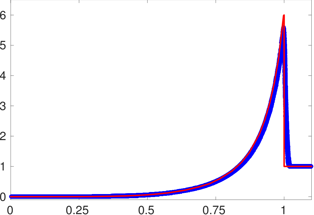
4.3 Sedov blast wave
This example is a simple one-dimensional model of an explosion that is difficult to simulate without aggressive (or positivity-preserving) limiting. The initial conditions involve one central cell with a large amount of energy buildup that is surrounded by a large area of undisturbed air. These initial conditions are supposed to approximate a delta function of energy. As time advances, a strong shock waves emanates from this central region and they move in opposite directions. This leaves the central post-shock regime with near zero density.
The initial conditions are uniform in both density and velocity, with and . The energy takes on the value in the central cell and in every other cell. This problem is explored extensively by Sedov, and in his classical text gives an exact solution that we use to construct the exact solution underneath our simulation [40]. We show our solution in Figure 5, and we point out that our results are quite good especially since we use such a coarse resolution of size .
4.4 Two dimensional examples
Here, we highlight the fact that this solver is able to operate on both Cartesian and unstructured meshes.
4.4.1 Convergence Results
We first verify the high-order accuracy of the proposed scheme. For problems where the density and pressure are far away from zero, the limiters proposed in this work “turn off”, and therefore have no effect on the solution. In order to investigate the effect of this positivity preserving limiter, we simulate a smooth problem where the solution has regions that are nearly zero. This is similar to the smooth test case considered by [47], [39] and [9]. To this end, we consider initial conditions defined by
| (86) |
on a computational domain of . We integrate this problem up to a final time of , and compute -norm errors against the exact solution given by
| (87) |
Results for Cartesian as well as unstructured meshes are presented in Table 1. These indicate that the high-order accuracy of the method is not sacrificed when the limiters are turned on. As a final note, we observe that it appears that in general much higher resolution is required on unstructured meshes before the numerical results enter the asymptotic regime.
| # Cartesian cells | Error | Order | # triangular cells | Error | Order |
|---|---|---|---|---|---|
| — | — | ||||
| — | — | — |
4.4.2 Sedov blast on an unstructured mesh
In this example we implement a two-dimensional version of the Sedov blast wave on the circular domain
The bulk of the domain begins with an undisturbed gas, , with uniform density , and near-zero energy . Only the cells at the center of the domain contain a large amount of energy that approximate a delta function. To simulate this, we introduce a small region at the center of the domain that is radially symmetric (because the simulation should be radially symmetric) of the form
where is a characteristic length of the mesh.
We present results in Figure 6 where we simulate our solution with a total of mesh cells.

4.4.3 Shock-diffraction over a block step: Cartesian mesh
This is a common example used to test positivity limiters [39, 47, 48]. It involves a Mach shock located above a step moving into air that is at rest with and . The domain this problem is typically solved on is . The step is the region . Our boundary conditions are transparent everywhere except above the step where they are inflow and on the surface of the step where we used solid wall. Our initial conditions have the shock located above the step at . The problem is typically run out to , and if a positivity limiter is not used the solution develops negative density and pressure values, which causes the simulation to fail. The solution shown in Figure 7 is run on a Cartesian mesh.
4.4.4 Shock-diffraction over a block step: unstructured mesh
Next, we run the same problem from §4.4.3, but we discretize space using an unstructured triangular mesh with cells. The results are shown in Figure 8, and indicate that the unstructured solver behaves similarly to the Cartesian one.
4.4.5 Shock-diffraction over a degree wedge
This final shock-diffraction test problem is very similar to the previous test problems, however it must be run on an unstructured triangular mesh because the wedge involved in this problem is triangular (with a degree angle) [49]. Our domain for this problem is given by
Again the boundary conditions are transparent everywhere except above the step where they are inflow and on the surface of the step where they are reflective solid wall boundary conditions. In addition, the initial conditions for this problem are also slightly different that those in the previous example. Here, we have a Mach shock located above the step at , and undisturbed air in the rest of the domain with and . This problem is run on an unstructured mesh with a total of cells. These results are presented in Figure 9.
5 Conclusions
In this work we developed a novel positivity-preserving limiter for the Lax-Wendroff discontinuous Galerkin (LxW-DG) method. Our results are high-order and applicable for unstructured meshes in multiple dimensions. Positivity of the solution is realized by leveraging two separate ideas: the moment limiting work of Zhang and Shu [48], as well as the flux corrected transport work of Xu and collaborators [45, 30, 9, 8, 39]. The additional shock capturing limiter, which is required to obtain non-oscillatory results, is the one recently developed by the current authors [31]. Numerical results indicate the robustness of the method, and are promising for future applications to more complicated problems such as the ideal magnetohydrodynamics equations. Future work includes introducing source terms to the solver, as well as pushing these methods to higher orders (e.g., -order), but that requires either (a) an expedited way of computing higher derivatives of the solution, or (b) rethinking how Runge-Kutta methods are applied in a modified flux framework (e.g., [7]).
Acknowledgements.
The work of SAM was supported in part by NSF grant DMS–1216732. The work of JAR was supported in part by NSF grant DMS–1419020.
References
- [1] P. Bochev, D. Ridzal, G. Scovazzi, and M. Shashkov. Formulation, analysis and numerical study of an optimization-based conservative interpolation (remap) of scalar fields for arbitrary Lagrangian-Eulerian methods. J. Comput. Phys., 230(13):5199–5225, 2011.
- [2] D.L. Book. Finite-difference techniques for vectorized fluid dynamics calculations. New York and Berlin, Springer-Verlag, 1981. 233 p, 1, 1981.
- [3] D.L. Book, J.P. Boris, and K. Hain. Flux-corrected transport II: Generalizations of the method. Journal of Computational Physics, 18(3):248–283, 1975.
- [4] J.P. Boris and D.L. Book. Flux-corrected transport. I. SHASTA, A fluid transport algorithm that works. Journal of computational physics, 11(1):38–69, 1973.
- [5] J.P. Boris and D.L. Book. Flux-corrected transport. III. Minimal-error FCT algorithms. Journal of Computational Physics, 20(4):397–431, 1976.
- [6] A.J. Christlieb, X. Feng, D.C. Seal, and Q. Tang. A high-order positivity-preserving single-stage single-step method for the ideal magnetohydrodynamic equations. arXiv preprint arXiv:1509.09208, 2015.
- [7] A.J. Christlieb, Y. Güçlü, and D.C. Seal. The Picard integral formulation of weighted essentially nonoscillatory schemes. SIAM J. Numer. Anal., 53(4):1833–1856, 2015.
- [8] A.J. Christlieb, Y. Liu, Q. Tang, and Z. Xu. High order parametrized maximum-principle-preserving and positivity-preserving WENO schemes on unstructured meshes. J. Comput. Phys., 281:334–351, 2015.
- [9] A.J. Christlieb, Y. Liu, Q. Tang, and Z. Xu. Positivity-preserving finite difference weighted ENO schemes with constrained transport for ideal magnetohydrodynamic equations. SIAM J. Sci. Comput., 37(4):A1825–A1845, 2015.
- [10] B. Cockburn, S. Hou, and C.-W. Shu. The Runge-Kutta local projection discontinuous Galerkin finite element method for conservation laws. IV. The multidimensional case. Math. Comp., 54(190):545–581, 1990.
- [11] B. Cockburn, G.E. Karniadakis, and C.-W. Shu. The development of discontinuous Galerkin methods. In Discontinuous Galerkin methods (Newport, RI, 1999), volume 11 of Lect. Notes Comput. Sci. Eng., pages 3–50. Springer, Berlin, 2000.
- [12] B. Cockburn, S.Y. Lin, and C.-W. Shu. TVB Runge-Kutta local projection discontinuous Galerkin finite element method for conservation laws. III. One-dimensional systems. J. Comput. Phys., 84(1):90–113, 1989.
- [13] B. Cockburn and C.-W. Shu. TVB Runge-Kutta local projection discontinuous Galerkin finite element method for conservation laws. II. General framework. Math. Comp., 52(186):411–435, 1989.
- [14] B. Cockburn and C.-W. Shu. The Runge-Kutta discontinuous Galerkin method for conservation laws. V. Multidimensional systems. J. Comput. Phys., 141(2):199–224, 1998.
- [15] R. Courant, E. Isaacson, and M. Rees. On the solution of nonlinear hyperbolic differential equations by finite differences. Comm. Pure. Appl. Math., 5:243–255, 1952.
- [16] M. Dumbser, D.S. Balsara, E.F. Toro, and C.-D. Munz. A unified framework for the construction of one-step finite volume and discontinuous Galerkin schemes on unstructured meshes. J. Comput. Phys., 227(18):8209–8253, 2008.
- [17] M. Dumbser, M. Käser, and E.F. Toro. An arbitrary high-order discontinuous galerkin method for elastic waves on unstructured meshes-v. local time stepping and p-adaptivity. Geophysical Journal International, 171(2):695–717, 2007.
- [18] M. Dumbser and C.-D. Munz. ADER discontinuous Galerkin schemes for aeroacoustics. Comptes Rendus Mécanique, 333(9):683–687, 2005.
- [19] M. Dumbser and C.-D. Munz. Building blocks for arbitrary high order discontinuous Galerkin schemes. J. Sci. Comput., 27(1-3):215–230, 2006.
- [20] M. Dumbser, O. Zanotti, A. Hidalgo, and D.S. Balsara. ADER-WENO finite volume schemes with space-time adaptive mesh refinement. J. Comput. Phys., 248:257–286, 2013.
- [21] G. Gassner, M. Dumbser, F. Hindenlang, and C.-D. Munz. Explicit one-step time discretizations for discontinuous Galerkin and finite volume schemes based on local predictors. J. Comput. Phys., 230(11):4232–4247, 2011.
- [22] S.K. Godunov. Difference method of computation of shock waves. Uspehi Mat. Nauk (N.S.), 12(1(73)):176–177, 1957.
- [23] S. Gottlieb, C.-W. Shu, and E. Tadmor. Strong stability-preserving high-order time discretization methods. SIAM Rev., 43(1):89–112 (electronic), 2001.
- [24] W. Guo, J.-M. Qiu, and J. Qiu. A new Lax–Wendroff discontinuous Galerkin method with superconvergence. J. Sci. Comput., 65(1):299–326, 2015.
- [25] A. Harten and G. Zwas. Self-adjusting hybrid schemes for shock computations. Journal of Computational Physics, 9(3):568–583, 1972.
- [26] J.F.B.M. Kraaijevanger. Contractivity of Runge-Kutta methods. BIT, 31(3):482–528, 1991.
- [27] D. Kuzmin and R. Löhner, editors. Flux-corrected transport. Scientific Computation. Springer-Verlag, Berlin, 2005. Principles, algorithms, and applications.
- [28] P. Lax and B. Wendroff. Systems of conservation laws. Comm. Pure Appl. Math., 13:217–237, 1960.
- [29] P.D. Lax. Weak solutions of nonlinear hyperbolic equations and their numerical computation. Comm. Pure Appl. Math., 7:159–193, 1954.
- [30] C. Liang and Z. Xu. Parametrized maximum principle preserving flux limiters for high order schemes solving multi-dimensional scalar hyperbolic conservation laws. J. Sci. Comput., 58(1):41–60, 2014.
- [31] S.A. Moe, J.A. Rossmanith, and D.C. Seal. A simple and effective high-order shock-capturing limiter for discontinuous Galerkin methods. arXiv preprint arXiv:1507.03024v1, 2015.
- [32] J. Von Neumann and R.D. Richtmyer. A method for the numerical calculation of hydrodynamic shocks. J. Appl. Phys., 21:232–237, 1950.
- [33] B. Perthame and C.-W. Shu. On positivity preserving finite volume schemes for Euler equations. Numer. Math., 73(1):119–130, 1996.
- [34] J. Qiu, M. Dumbser, and C.-W. Shu. The discontinuous Galerkin method with Lax-Wendroff type time discretizations. Comput. Methods Appl. Mech. Eng., 194(42-44):4528–4543, 2005.
- [35] J.A. Rossmanith. DoGPack software, 2015. Available from http://www.dogpack-code.org.
- [36] S.J. Ruuth and R.J. Spiteri. Two barriers on strong-stability-preserving time discretization methods. In Proceedings of the Fifth International Conference on Spectral and High Order Methods (ICOSAHOM-01) (Uppsala), volume 17, pages 211–220, 2002.
- [37]
D.C. Seal.
FINESS software, 2015.
Available from
https://bitbucket.org/dseal/finess. - [38] D.C. Seal, Y. Güçlü, and A.J. Christlieb. High-order multiderivative time integrators for hyperbolic conservation laws. J. Sci. Comput., 60(1):101–140, 2014.
- [39] D.C. Seal, Q. Tang, Z. Xu, and A.J. Christlieb. An explicit high-order single-stage single-step positivity-preserving finite difference WENO method for the compressible Euler equations. Journal of Scientific Computing, pages 1–20, 2015.
- [40] L.I. Sedov. Similarity and dimensional methods in mechanics. Academic Press, New York-London, 1959.
- [41] G.A. Sod. A survey of several finite difference methods for systems of nonlinear hyperbolic conservation laws. J. Computational Phys., 27(1):1–31, 1978.
- [42] A. Taube, M. Dumbser, D.S. Balsara, and C.-D. Munz. Arbitrary high-order discontinuous Galerkin schemes for the magnetohydrodynamic equations. J. Sci. Comput., 30(3):441–464, 2007.
- [43] V.A. Titarev and E.F. Toro. ADER: arbitrary high order Godunov approach. In Proceedings of the Fifth International Conference on Spectral and High Order Methods (ICOSAHOM-01) (Uppsala), volume 17, pages 609–618, 2002.
- [44] P.A. Ullrich and M.R. Norman. The flux-form semi-Lagrangian spectral element (FF–SLSE) method for tracer transport. Quarterly Journal of the Royal Meteorological Society, 140(680):1069–1085, 2014.
- [45] Z. Xu. Parametrized maximum principle preserving flux limiters for high order schemes solving hyperbolic conservation laws: One-dimensional scalar problem. Math. Comp., 83(289):2213–2238, 2014.
- [46] S.T. Zalesak. The design of flux-corrected transport (FCT) algorithms for structured grids. In Flux-corrected transport, Sci. Comput., pages 29–78. Springer, Berlin, 2005.
- [47] X. Zhang and C.-W. Shu. On positivity preserving high order discontinuous Galerkin schemes for compressible Euler equations on rectangular meshes. J. Comp. Phys., 229:8918—8934, 2010.
- [48] X. Zhang and C.-W. Shu. Maximum-principle-satisfying and positivity-preserving high-order schemes for conservation laws: survey and new developments. Proc. R. Soc. A, 467(2134):2752–2776, 2011.
- [49] X. Zhang, Y. Xia, and C.-W. Shu. Maximum-principle-satisfying and positivity-preserving high order discontinuous Galerkin schemes for conservation laws on triangular meshes. J. Sci. Comput., 50(1):29–62, 2012.
- [50] H. Zheng, Z. Zhang, and E. Liu. Non-linear seismic wave propagation in anisotropic media using the flux-corrected transport technique. Geophysical Journal International, 165(3):943–956, 2006.