Space-Time Index Modulation
Abstract
In this paper, we present a new multi-antenna modulation scheme, termed as space-time index modulation (STIM). In STIM, information bits are conveyed through antenna indexing in the spatial domain, slot indexing in the time domain, and -ary modulation symbols. A time slot in a given frame can be used or unused, and the choice of the slots used for transmission conveys slot index bits. In addition, antenna index bits are conveyed in every used time slot by activating one among the available antennas. -ary symbols are sent on the active antenna in a used time slot. We study STIM in a cyclic-prefixed single-carrier (CPSC) system in frequency-selective fading channels. It is shown that, for the same spectral efficiency and single transmit RF chain, STIM can achieve better performance compared to conventional orthogonal frequency division multiplexing (OFDM). Low-complexity iterative algorithms for the detection of large-dimensional STIM signals are also presented.
Keywords – Space-time index modulation, multi-antenna systems, RF chain, single-carrier systems, OFDM, low-complexity detection.
I Introduction
Multi-antenna multiple-input multiple-output (MIMO) wireless systems are known to provide increased spectral and power efficiencies. Recently, various index modulation based schemes have been developed for MIMO systems to improve the achievable rate and performance with reduced hardware complexity [1]-[6]. Spatial modulation (SM) scheme performs index modulation in the spatial domain [1]. SM activates only one transmit antenna among the available transmit antennas in any given channel use. Thus, SM reduces hardware complexity by using only one transmit radio frequency (RF) chain. The index of the active antenna used for transmission conveys information bits. SM was generalized to activate multiple transmit RF chains in a given channel use, which was termed as the generalized spatial modulation (GSM) [2], [3]. It has been shown that GSM outperforms conventional MIMO systems in terms of bit error performance for a given spectral efficiency [7].
Index modulation has been exploited in domains other than the spatial domain. Indexing subcarriers in multicarrier systems like OFDM, termed as subcarrier index modulation (SIM) [4],[5], is an example of index modulation in the frequency domain. Generalized space-frequency index modulation (GSFIM) reported in [6], [8] combines the benefits of indexing over spatial and frequency domains. In GSFIM, information bits are conveyed through antenna indexing, subcarrier indexing, and modulation symbols. However, GSFIM system does not employ antenna indexing in every channel use. The indices of the active antennas are fixed in a given GSFIM frame. This limits the rate achievable through antenna indexing. Generalized space-time shift keying (GSTSK) reported in [9] performs indexing of space-time dispersion matrices. In GSTSK, the sum of a subset of all possible space-time dispersion matrices are chosen for transmission in a certain number of channel uses. The choice of this subset conveys information bits.
In this paper, we propose a new index modulation scheme, referred to as space-time index modulation (STIM). STIM efficiently performs indexing in spatial and time domains. In STIM, transmission is carried out in frames. Each frame consists of certain number of time slots. Not all the time slots in a frame are necessarily used for transmission (i.e., no transmission takes place in certain time slots). In fact, the choice of the combination of used slots and unused slots in a frame conveys information bits through time slot indexing. On the used time slots, modulation symbols are sent on the transmit antenna chosen based on antenna index bits. Thus, information bits are conveyed through indices of the used time slots, index of the active antenna, and modulation symbols.
STIM is well suited for use in block transmission schemes. For example, STIM can be used in cyclic-prefixed single-carrier (CPSC) scheme [10], which is a block transmission scheme suited for inter-symbol interference (ISI) channels. In this context, the following two questions arise:
- 1.
how does STIM used in a CPSC scheme compare in terms of rate and performance relative to conventional OFDM in ISI channels, and
- 2.
how to detect STIM signals, particularly when the dimensionality (i.e., frame size) is large.
While the first question is aimed at seeing if there are benefits vis-a-vis conventional schemes, the second question is aimed at addressing the implementation complexity issue. This paper presents answers to the above questions. First, it is found that, for the same spectral efficiency and single transmit RF chain, STIM in CPSC can outperform conventional OFDM. Second, low-complexity STIM detection algorithms which scale well for large dimensions are proposed. These results suggest that STIM can be a promising modulation scheme, and has the potential for further investigations beyond what is reported in this paper.
The rest of this paper is organized as follows. In Sec. II, we present the STIM scheme, system model, and rate analysis. The proposed low-complexity algorithms for STIM signal detection are presented in Sec. III. Bit error performance results and discussions are presented in Sec. IV. Conclusions and scope for future work are presented in Sec. V.

II STIM system model
The STIM scheme has transmit antennas with a single transmit RF chain (i.e., , where is the number of transmit RF chains), and receive antennas. The channel is assumed to be frequency-selective with multipaths11 1 The multipath delays can take generic delay values. As a result of Nyquist sampling at the receiver, the path delays can be reduced to integer multiples of the signaling interval [11]. The powers of the channel gains at each integer multiple of the signaling interval is given by the power-delay profile (PDP). The PDP of the frequency selective fading channel captures the statistical characteristics and dependencies between the various multipaths of the channel [11]. We consider an exponential PDP as described in Sec. II-D.. Transmission is carried out in frames. Each frame consists of channel uses, where denotes the length of the data part in number of channel uses and channel uses are used for transmitting cyclic prefix (CP). Information bits are conveyed through three different entities, namely, indices of the used time slots in a frame, and index of the active transmit antenna in a channel use, and symbols from a modulation alphabet , as follows.
II-A Time slot indexing
We have time slots in a frame available for conveying information. Among these slots, only slots are selected for transmission of modulation symbols. Let denote the alphabet from which the modulation symbols are drawn. There are possibilities of choosing which slots are used and which slots are not used. Specifically, a time slot is said to be used if any one of the antennas transmits a symbol from in that slot. A slot is said to be not used, if none of the antennas transmit in that slot (i.e., all antennas remain silent, where silence can be viewed as sending a 0). The slots used for transmission in a given frame are chosen based on information bits. Let us call a given realization of the used/unused status of slots in a frame as a ‘slot activation pattern (SAP)’. Out of possible SAPs, only SAPs are used for slot indexing to convey bits.
Example: Let , . So, and slot index bits. The possible SAPs here are:
where 1’s correspond to the location of the used time slots and 0’s correspond to the location of the unused time slots. Each used slot carries one symbol from , and nothing gets transmitted in unused slots.
II-B Antenna indexing
A transmit antenna is said to be active in a given channel use if it transmits a non-zero modulation symbol in that channel use. Similarly, a transmit antenna is said to be inactive if it does not transmit any modulation symbol in that channel use. The transmit antenna activated in a given channel use is chosen based on information bits. Note that in an STIM frame, in each of the used time slots the index of the active antenna can be different. In the remaining slots, all the transmit antennas are inactive. Since only out of time slots are used in an STIM frame, information bits are conveyed through antenna indices in one STIM frame.
With the addition of antenna indexing, the chosen SAP in a given frame gets mapped on to a space-time activation matrix of dimension , whose entries are zeros and ones; means a symbol from is sent on the th antenna in the th slot, , and ; means 0 is sent on the th antenna in the th slot (i.e., th slot is unused). Note that only columns in will have a non-zero entry and the remaining columns will have only zero entries.
Example: Let = 2, , . The possible ‘antenna activation patterns (AAP)’ are given by , where a 1 corresponds to the index of the active antenna, and a 0 corresponds to the index of the inactive antenna. Therefore, bit can be conveyed through the index of the active antenna in each of the used slots.
Let denote the STIM signal matrix without CP. The matrix is formed by using symbols from in those entries of the matrix where . Now, the STIM signal matrix with CP, denoted by and of size , is formed by appending CP symbols to . The columns of are transmitted in channel uses.
Example: Consider a system with , and 4-QAM. Let denote a possible input information bit sequence to be transmitted by the STIM transmitter. The first bits choose the index of the active antennas in the used time slots. The next bits choose the indices of the seven used time slots. The last bits choose the seven 4-QAM symbols. For this input bit sequence, the matrix can be
and the corresponding matrix is
where . The STIM signal matrix with CP appended is then given by
The block diagram of STIM transmitter is shown in Fig. 1.
II-C Analysis of achieved rate in STIM
In this subsection, we analyze the achieved rate in STIM. We also compare the rates achieved in STIM and conventional OFDM, both using a single transmit RF chain. Based on the description of STIM in the previous subsection, the achieved rate in STIM can be written as
| (1) | |||||
Note that in conventional OFDM, there are no slot and antenna index bits to contribute to the achieved rate. All the subcarriers carry modulation symbols. The achieved rate in OFDM with subcarriers is given by
| (2) |
From (1) and (2), we can write the percentage of rate improvement offered by STIM over OFDM as
| (3) |
II-C1 Maximizing over
Define and . From (1), the achieved rate in STIM as a function of can be written as
| (4) |
We need to obtain a that maximizes . The combinatorial nature of the expression for makes it difficult to obtain the value of that maximizes through differentiation technique. Thus, we try to obtain a range of values for over which is maximized.
Let be a value of for which is maximum. Since is a concave function22 2 It is known that is concave w.r.t and is a monotone function. Therefore, from (4), is a concave function w.r.t ., should satisfy
| (5) | |||||
| (6) |
Expanding (5), we write
| (7) |
Define . From (7), an upper bound for can be written as
| (8) |
Next, we obtain a lower bound by expanding (6) as follows:
| (9) |
Now, a lower bound for can be written as
| (10) |
From (7) and (10), we can see that any such that will maximize . The bounds and are considerably tight. This can be seen by
| (11) |
Therefore, maximum rate can be achieved in STIM when we choose the value of to be , where
| (12) |
II-C2 Maximizing over
From (1), (2), and (3), the percentage rate improvement can be written as
| (13) |
Let us assume33 3 This assumption can be reasoned as follows: for large values of , from (10), the value of can be approximated to the nearest integer as . Further, this can be observed in Fig. 2, where, as (or alternatively ) increases, the value of for which the maximum rate is achieved increases and tends towards . . Now, (13) can be written as
To maximize with respect to , we evaluate :
| (14) |
Therefore, the percentage of rate improvement obtained through STIM over OFDM can be maximized when the number of slots .
II-C3 Numerical results
In Fig. 2, we plot the variation of the achieved rate of STIM as a function of . This figure shows the values of for varying , , (i.e., ), , , and (i.e., ). It can be seen that the STIM rate is maximized only by certain values of . Further, the values of given by (12) coincide with the values of that maximize . For , the values of are , respectively.


In Fig. 3, we plot as a function of . This figure presents the values of for ) (i.e., ), and (i.e., ), ) (), and (), ) (), and (), and ) (), and (). The value of obtained through simulation, that maximizes , matches well with the analytical expression given by (14). For the system parameters considered in Fig. 3, is maximum at ) , ) , ) , and ) .
II-D Received STIM signal
Now, let us write the received STIM signal model at the receiver. Let denote the channel gain from th transmit antenna to the th receive antenna on the th multipath. The power delay profile of the channel is assumed to follow exponential decaying model, i.e., , . Let denote the transmitted symbol vector of size in the th channel use, . Note that is the th column of the matrix . We assume that the channel remains invariant in one STIM frame duration. At the receiver, after removing the cyclic prefix, the received vector can be represented as
| (15) |
where is the noise vector of size with , is the vector of size given by , and is the equivalent block circulant channel matrix given by
where is the channel matrix corresponding to the th multipath. Assuming perfect knowledge of at the receiver, the maximum likelihood (ML) detection rule is given by
| (16) |
where denotes the set of all possible vectors.
III Low-complexity STIM detection
From (16), it can be seen that the ML detection of an STIM frame has a complexity that increases exponentially with , . In order to enable the detection of large dimensional STIM signals, in this section, we present two low-complexity detection algorithms using message passing.
III-A Two-stage STIM detector
In this proposed two-stage STIM detector (2SSD), detection is carried out in two stages. The first stage is a minimum mean square error (MMSE) estimator, which is followed by a message passing based detector. The purpose of the first stage detection is to provide an estimate of the indices of the active antennas in the STIM frame. Using this estimate, the message passing based detector obtains an estimate of the indices of the used time slots in the frame and the modulation symbols. Finally, these estimates are demapped to obtain an estimate of the transmitted information bit sequence.
Stage 1 : The first stage detection is performed using MMSE estimator as
| (17) |
where is of the form . We construct the index set , where is the index of the element with the largest magnitude in , and . The set gives the estimates of the indices of the active antennas in the channel uses of an STIM frame. Now, we can write (15) in the form
| (18) |
where is an vector whose elements correspond to the elements in at the indices given by the set , and is the channel matrix obtained by choosing the columns of at the indices given by the set .
Stage 2: The second stage of the 2SSD algorithm is a message passing based algorithm that works on the model given by (18). The message passing algorithm gives the estimates of the indices of the used time slots and the modulation symbols.
Let be the time slot activity indicator variable for the th time slot. That is, whenever th time slot is used, and otherwise. The th time slot corresponds to the th entry of vector . Note that . This is referred to as the STIM time constraint . Let . We obtain the a posteriori probabilities (APP) of the elements of and , using which the time slot index bits and the modulation symbol bits are estimated.

Figure 4 shows the graphical model for message passing. The graph consists of four sets of nodes. Messages are exchanged between these nodes in two layers: one corresponding to the probabilities of the modulation symbols and the other corresponding to the probabilities of the time slot activity indicators. For the system described in (18), the a posteriori probability is given by
| (19) | |||||
The graph is constructed so as to marginalize the above probability distribution. The following four sets of nodes are defined: observation nodes corresponding to the elements of , variable nodes corresponding to the elements of , ) time slot activity nodes corresponding to the elements of , and a constraint node corresponding to the time constraint . The messages that are exchanged in layer 1 between the observation and the variable nodes produce approximate APPs of the individual elements of . The messages that are exchanged in layer 2 between the time slot activity nodes and the STIM time constraint node generate the APPs of the elements of . To generate these messages, we employ a Gaussian approximation of interference as follows. We write the th element of as
| (20) |
where and . We approximate to be Gaussian with mean and variance , which are calculated as
| (21) |
and
| (22) |
The messages passed between the nodes are given below.
Layer 1: The message computed at the observation node is
| (23) | |||||
where . The APP of the individual elements of is obtained at the variable nodes as
| (24) | |||||
where denotes the set of all elements of except , and if , and if .
Layer 2: The APP estimate of from the variable nodes are computed as
| (25) | |||||
The APP estimate of computed at the time slot activity nodes after processing the STIM time constraint is
| (26) | |||||
where denotes the probability that the time slot activity pattern satisfies the STIM time constraint given that the th time slot is used, and denotes the probability that the time slot activity pattern satisfies given that the th time slot is unused. This probability is evaluated as , where is the convolution operator, and is a probability mass function with probability masses at points . The messaging passing algorithm is summarized as follows.
- 1.
Initialize , , , .
- 2.
Compute , .
- 3.
Compute , .
- 4.
Compute , .
- 5.
Compute , .
The above steps are repeated for a fixed number of iterations. Damping of the messages ’s and ’s is done using a damping factor in each iteration [12]. At the end of the iterations, an estimate of the index of the used time slots are obtained by choosing the time slots that have the largest APP. That is, a set is obtained such that are the largest APP values of . These estimates are demapped to get the time slot index bits. Since the transmit antennas are activated only in time slots, the antenna indices from the set that correspond to the used time slot estimates are chosen and demapped to obtain the antenna index bits. Finally, from ’s, the information bits corresponding to the modulation symbols are obtained.
III-B Three-stage STIM detector
In this subsection, we present another detection algorithm called three-stage STIM detection (3SSD) algorithm, where the first two stages are the same as those in 2SSD. The third stage in the 3SSD aims to further improve the reliability of the estimated antenna index bits and the modulation symbol bits through the use of message passing over a bipartite (factor) graph. The estimates of the indices of the used time slots (i.e., the set ) obtained from the second stage are fed as input to the third stage. The third stage achieves improved performance compared to 2SSD without much increase in complexity. The message passing scheme for the third stage is described below.
Let denote the set of all possible vectors that could be transmitted by the STIM transmitter in an used time slot. Therefore, . For example, for and BPSK, the set is given by
Let be the -length vector transmitted in the th used time slot, and . Let be an matrix obtained by choosing columns of the channel matrix corresponding to the estimated indices of the used time slots given by the set . Now, the received signal can be expressed as
| (27) |
The third stage message passing works on the system model in (27), and estimates , given and . The graphical model of this scheme consists of variable nodes each corresponding to a , and observation nodes each corresponding to a . This graphical model is illustrated in Fig. 5.
The messages passed between the variable nodes and the observation nodes are constructed as follows. From (27), the received signal can be written as
| (28) |
where is a row vector of length given by , and is the -length vector transmitted in the th used time slot. We approximate to be Gaussian with mean and variance , where
| (29) |
and
| (30) | |||||
where denotes the a posteriori probability message computed at the variable nodes as
| (31) |
The message passing schedule is as follows.
- 1.
Initialize , .
- 2.
Compute , and .
- 3.
Compute , .
Steps 2 and 3 are repeated for a fixed number of iterations. Damping of the messages ’s is done using a damping factor in each iteration. At the end of the iterations, the vector probabilities are computed as
| (32) |
The estimates s are obtained by choosing the signal vector that has the largest APPs. That is,
| (33) |
The estimate of the active antenna index in the th used time slot is obtained from , which is then demapped to obtain the antenna index bits. The non-zero entries of are demapped to get the modulation symbol bits. The indices in set are demapped to get the slot index bits.

IV Results and discussions
In this section, we present the bit error rate (BER) performance of the proposed STIM detection algorithms. We compare the performance of STIM with that of OFDM. It is noted that both STIM and OFDM use a single transmit RF chain (i.e., for STIM and OFDM). We consider a frequency-selective channel with and exponential power delay profile presented in Sec. II-D.
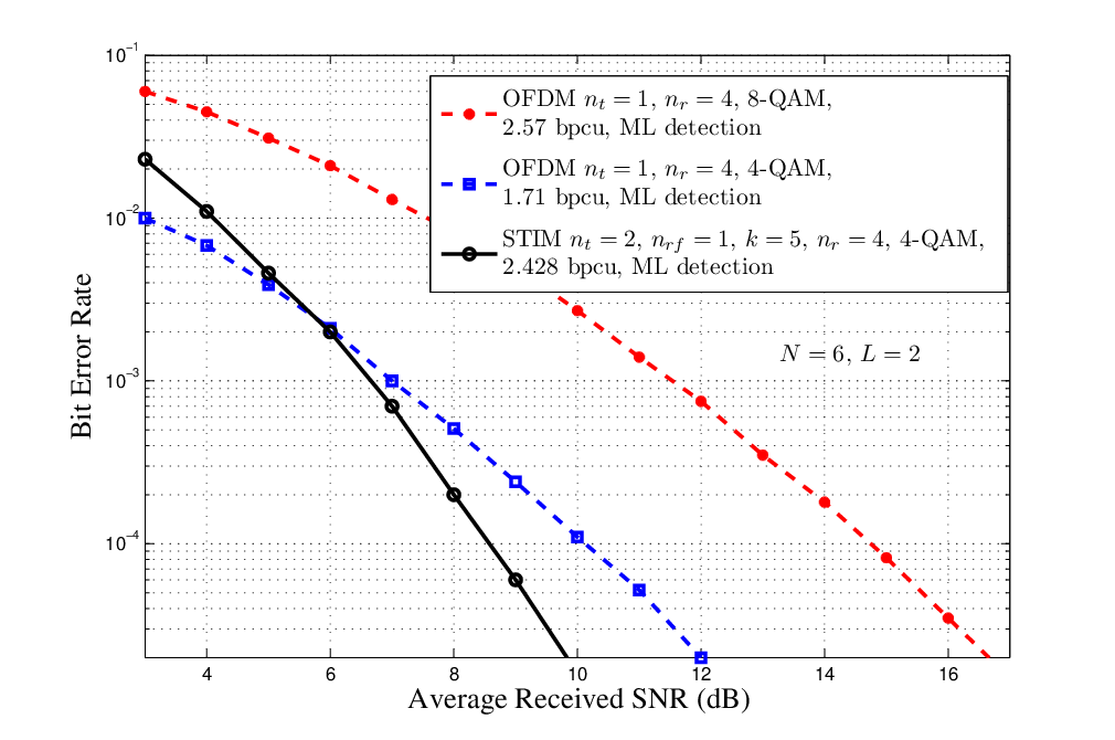
In Fig. 6, we present the maximum likelihood (ML) performance of the STIM system with 4-QAM, and a spectral efficiency of 2.428 bpcu. We compare this performance with that of conventional OFDM. The OFDM systems considered for comparison are: , 8-QAM, and spectral efficiency of 2.57 bpcu, and , 4-QAM, and spectral efficiency of 1.71 bpcu. From Fig. 6, we observe that the STIM system outperforms the conventional OFDM systems. At a BER of BER, STIM outperforms OFDM with 2.57 bpcu by about 6 dB, and OFDM with 1.71 bpcu by about 1.2 dB. This shows that STIM can achieve better performance than the conventional OFDM scheme as well as provide higher rate through transmit antenna and time slot indexing.
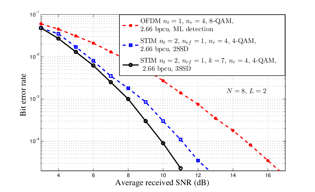
In Fig. 7, we present the BER performance of STIM detected using the proposed 2SSD and 3SSD algorithms. The value of the damping factor used is . The STIM system considered has , , , , 4-QAM, and 2.66 bpcu spectral efficiency. For comparison purposes, we also present the performance of conventional OFDM with the same spectral efficiency of 2.66 bpcu, using the following system parameters: , , , and 8-QAM. From Fig. 7, we see that the performance of STIM with 2SSD algorithm is better than OFDM with ML detection by about 3.7 dB at a BER of . We also see that STIM with 3SSD algorithm outperforms OFDM with ML detection by about 4.7 dB at a BER of . The performance of 3SSD algorithm is better than that of the 2SSD algorithm by about 1 dB at a BER of . This is because the third stage message passing in 3SSD improves the reliability of the detected information bits. In Fig. 8, a similar performance gain in favor of STIM is observed for at 2.769 bpcu.

V Conclusion
We proposed a new modulation scheme referred to as the space-time index modulation (STIM). This modulation scheme conveys information bits through indexing of antennas and time slots, in addition to -ary modulation symbols. This enables STIM to achieve high spectral efficiencies. We showed that, for the same spectral efficiency and single transmit RF chain, STIM can achieve better performance than conventional OFDM in frequency-selective fading channels. We also proposed two low-complexity detection algorithms which scale well for large dimensions. STIM with the proposed detection algorithms was shown to outperform conventional OFDM. STIM, therefore, can be a promising modulation scheme, and has the potential for further investigations beyond what is reported in this paper. For example, generalization of indexing in both space and time with more than one transmit RF chain can be investigated as future extension to this work. Also, diversity analysis of STIM and its generalized schemes is another important topic for further investigations.
References
- [1] M. Di Renzo, H. Haas, A. Ghrayeb, S. Sugiura, and L. Hanzo, “Spatial modulation for generalized MIMO: challenges, opportunities and implementation,” Proc. of the IEEE, vol. 102, no. 1, pp. 56-103, Jan. 2014.
- [2] J. Wang, S. Jia, and J. Song, “Generalised spatial modulation system with multiple active transmit antennas and low complexity detection scheme,” IEEE Trans. Wireless Commun., vol. 11, no. 4, pp. 1605-1615, Apr. 2012.
- [3] T. Datta and A. Chockalingam, “On generalized spatial modulation,” Proc. IEEE WCNC’2013, pp. 2716-2721, Apr. 2013.
- [4] R. Abu-alhiga and H. Haas, “Subcarrier-index modulation OFDM,” Proc. IEEE PIMRC’2009, pp. 177-181, Sep. 2009.
- [5] E. Basar, U. Aygolu, E. Panayirci, and H. V. Poor, “Orthogonal frequency division multiplexing with index modulation,” Proc. IEEE GLOBECOM’2012, pp. 4741-4746, Dec. 2012.
- [6] T. Datta, H. Eshwaraiah, and A. Chockalingam, “Generalized space and frequency index modulation,” IEEE Trans. Veh. Tech., vol. 65, no. 7, pp.4911-4924, Jul. 2016.
- [7] T. L. Narasimhan, P. Raviteja, and A. Chockalingam, “Generalized spatial modulation in large-scale multiuser MIMO systems,” IEEE Trans. Wireless Commun., vol. 14, no. 7, pp. 3764-3779, Jul. 2015.
- [8] B. Chakrapani, T. L. Narasimhan, and A. Chockalingam, “Generalized space and frequency index modulation: Low complexity encoding and detection,” Proc. IEEE GLOBECOM’2015, Dec. 2015.
- [9] S. Sugiura, S. Chen, and L. Hanzo, “Generalized space-time shift keying designed for flexible diversity-, multiplexing- and complexity-tradeoffs,” IEEE Trans. Wireless Commun., vol. 10, no. 4, pp. 1144-1153, Apr. 2011.
- [10] Z. Wang, X. Ma, and G. B. Giannakis, “OFDM or single-carrier block transmissions?,” IEEE Trans. Commun., vol. 52, no. 3, pp. 380-394, Mar. 2004.
- [11] D. Tse and P. Viswanath, Fundamentals of Wireless Communications, Cambridge Univ. Press, 2005.
- [12] M. Pretti, “A message passing algorithm with damping,” J. Statist. Mech.: Theory Practice, p. 11008, Nov. 2005.