Stellar modelling of Spica, a high-mass spectroscopic binary with a Cep variable primary componentThanks: Based on data from the MOST satellite, a Canadian Space Agency mission, jointly operated by Dynacon Inc., the University of Toronto Institute for Aerospace Studies and the University of British Columbia, with the assistance of the University of Vienna.
Abstract
Binary stars provide a valuable test of stellar structure and evolution, because the masses of the individual stellar components can be derived with high accuracy and in a model-independent way. In this work, we study Spica, an eccentric double-lined spectroscopic binary system with a Cep type variable primary component. We use state-of-the-art modelling tools to determine accurate orbital elements of the binary system and atmospheric parameters of both stellar components. We interpret the short-period variability intrinsic to the primary component, detected on top of the orbital motion both in the photometric and spectroscopic data. The non-LTE based spectrum analysis reveals two stars of similar atmospheric chemical composition consistent with the present day cosmic abundance standard defined by Nieva & Przybilla (2012). The masses and radii of the stars are found to be 11.431.15 M⊙ and 7.210.75 M⊙, and 7.470.54 R⊙ and 3.740.53 R⊙ for the primary and secondary, respectively. We find the primary component to pulsate in three independent modes, of which one is identified as a radial mode, while the two others are found to be non-radial, low degree modes. The frequency of one of these modes is an exact multiple of the orbital frequency, and the mode identification suggests a tidal nature for this particular mode. We find a very good agreement between the derived dynamical and evolutionary masses for the Spica system to within the observational errors of the measured masses. The age of the system is estimated to be 12.51 Myr.
Keywords:
binaries: spectroscopic — stars: individual ( Virginis) — stars: fundamental parameters — stars: variables: general — stars: oscillations1 Introduction
Spectroscopic binary stars provide a valuable test of stellar structure and evolution models since accurate, model-independent dynamical masses can be measured for the individual stellar components of a binary. Moreover, an existence of pulsating stars in binary systems allows the confrontation of the dynamical masses with those obtained from the asteroseismic analysis. Since the latter masses are model-dependent, pulsators in binary systems provide a test of the theory of stellar evolution and oscillations. Apart from that, massive stars in binary systems are known to suffer from the so-called mass discrepancy problem, which is important to investigate in the context of improving the current theories of stellar structure and evolution. The term mass discrepancy was first introduced by Herrero et al. (1992) and in its original formulation refers to the disagreement between the spectroscopic and evolutionary masses of the star. The evolutionary mass is the one estimated by fitting evolutionary tracks to a position of the star in the Hertzspung-Russel or - Kiel diagram, whereas the spectroscopic mass stands for the stellar mass computed from the spectroscopically derived value of the surface gravity and from the radius of the star. The radius is in turn calculated from the absolute visual magnitude of the star and the (effective temperature dependent) integral of stellar flux over the wavelength (Kudritzki, 1980, see). Thus, the definition of the mass discrepancy by Herrero et al. (1992) has nothing to do specifically with binary systems but refers to massive stars in general. We keep on using the term mass discrepancy in application to binary systems throughout the paper, and warn the reader that we refer to the discrepancy between the evolutionary masses and those inferred from binary dynamics (dynamical masses).
This paper is the third in a series and concerns a detailed investigation of Spica, a short-period double-lined spectroscopic binary containing a massive star, where we address the above mentioned problems. In the two previous studies, the double-lined spectroscopic binary systems V380 Cyg (Tkachenko et al., 2014a) and Scorpii (Tkachenko et al., 2014b) have been investigated. The asteroseismic modelling of the primary component of Sco was largely successful leading to the mass and radius determination to precisions of 10% or better, which is a factor of three more accurate than the corresponding values derived from the combined spectroscopic orbital and atmospheric parameters, and the interferometric orbital inclination angle (North et al., 2007, taken from). We have found an evidence of the mass discrepancy for the secondary component of the binary, i.e. the evolutionary models suggest higher mass than the one inferred from the binary dynamics. The study of V380 Cyg benefited from the fact that it is an eclipsing system with space-based photometry available, thus the dynamical masses and radii of the individual stellar components could be derived to precisions approaching 1% level. Both components of the binary were found to show significant discrepancy between the dynamical and evolutionary masses, leading us to the conclusion that the single star evolutionary models are inadequate for this particular system.


Spica (Vogel, 1890, mag, discovered to be a spectroscopic binary by) is an important system to study in the context of testing the current theories of stellar structure and evolution for massive stars, which are way more uncertain than the models for lower mass stars. The more evolved primary component is also known to be an intrinsically variable star that belongs to the class of Cep variables (Aerts et al., 2010, Chapter 2) and pulsates in pressure modes. As a consequence, the system was the subject of numerous studies addressing both the questions on configuration of the orbit as well as on the variability intrinsic to the primary component. For example, Shobbrook et al. (1972) used both the newly obtained and historical RV data to determine orbital parameters of the binary. The obtained solution was found to be in good agreement with the one reported by Herbison-Evans et al. (1971).
| Time period | ||
| Calendar date | JD (2 454 000+) | |
| 19.03–01.04.2007 | 178–191 | 772 |
| 18.04–30.04.2007 | 208–220 | 798 |
| 22.07–30.07.2007 | 304–312 | 161 |
| Total number of spectra: | 1731 | |
Despite the extensive investigations in the past, the oscillation behaviour of Spica is currently not well understood: several studies reported about irregular variability of the individual frequencies on short time scales, and there is quite some diversity in the reported frequencies the Spica system was found to pulsate in (see Sect. 6 for an overview). The fact that the system is eccentric and the intrinsic pulsations of the more evolved component are in the range below 6 d-1 (69.4 Hz) makes it an interesting target to search for pulsations that are resonantly driven by the dynamic tide. These so-called tidally induced pulsations (Aerts et al., 2010, Chapter 2) have so far been detected in BA main-sequence stars with masses below 5 (Welsh et al., 2011; Thompson et al., 2012; Hambleton et al., 2013; Pápics et al., 2013, e.g.,) but never in early B-type stars. Should this type of stellar oscillation be found in either of the stellar components of the Spica system, it will be the first massive binary in which resonantly driven oscillations have been detected. Such a detection would make Spica an important test case for the evolution of massive stars in binary systems as the tidally-induced pulsations are expected to play a significant role in angular momentum exchange between the orbit and the individual stellar components, and thus in the evolution of the orbital elements of the system with time.
Better observational constraints on the oscillation behaviour of Spica could be obtained if high-quality space-based were available for this star. Moreover, the system was also reported by Desmet et al. (2009) as possibly a grazingly eclipsing binary, so good quality observational data coupled to state-of-the-art analysis are required to detect a tiny eclipse signal, if present at all. A possible detection of the eclipses in the photometric data of the system could help to constrain the fundamental properties of the individual stellar parameters to a better precision than is currently available.
Overall, our study addresses several scientific questions at the same time. First of all, we aim at improving the understanding of the pulsational behaviour of the Spica system using and improved observational dataset, including high-quality photometric observations from space combined with high-quality high-resolution ground-based spectroscopy (see Sect.2). The orbital configuration of the system is determined in Sects. 3 and 4, with a particular interest in whether the star could be a grazingly eclipsing system. We also perform a detailed (atmospheric) chemical composition analysis for both stellar components of the binary (Sect. 5), which particularly allows us to see whether a increased nitrogen abundance at the surface of the star due to rotational mixing applies to the Spica system as reported in the literature (Hunter et al., 2008; Brott et al., 2011, e.g.,). The intrinsic variability of the more massive component of the Spica system is explored in detail in Sect. 6. This includes detailed frequency analysis, identification of the individual pulsation modes from spectroscopic data, and a search for observational signatures of tidally-induced pulsations. The possibility of detecting for the first time forced oscillations in a high-mass star (M⊙) defines the second scientific question we address in this study. Finally, we investigate the binary system in the context of the above-mentioned mass discrepancy problem by comparing the (spectroscopically inferred) positions of the individual stellar components in the - Kiel diagram with the evolutionary tracks (Sect. 7).
2 Observations and data reduction
We obtained 1731 high resolution (R = 50 000) high signal-to-noise ratio (S/N) spectra with the coralie spectrograph attached to the 1.2m Euler Swiss Telescope (La Silla, Chile). The data were gathered in three different runs, in March, April, and July 2007, and cover wide wavelength range between 381 and 681 nm. Table 1 gives the journal of our observations and lists calendar and Julian dates of the beginning and the end of the observing run, as well as the number of spectra that were obtained within each of the runs.
The spectroscopic data were reduced by means of a dedicated data reduction pipeline. The procedure included bias and stray-light subtraction, cosmic rays filtering, flat fielding, wavelength calibration by ThAr lamp, and order merging. Normalisation to the local continuum has been done by fitting a cubic spline function through some tens of carefully selected continuum points. The whole normalisation procedure as well as its implementation are described in more detail in Pápics et al. (2012).
Photometric data were gathered with the MOST space-based mission (Walker et al., 2003). The satellite is equipped with a 15-cm Rumak-Maksutov optical telescope feeding a CCD photometer. The Spica system was observed in the “Fabry mode” of MOST (Walker et al., 2003), and was sampled using 30 second exposures over a baseline of 22.92 days in March-April 2007. The single point precision is of the order of 1–2 mmag; the complete light curve of the system is illustrated in Fig. 1 (top panel). For the analysis, the light curve was converted to a magnitude scale; a small, long term instrumental trend has been removed by fitting a second-order degree polynomial to the entire data set.
The observational data set we analyse in this study is unique in the sense that 1) photometric data were obtained for the Spica system from space for the first time and are expected to provide much better constraints on the orbital configuration of the system and on the intrinsic variability of the individual stellar components; 2) the photometric data are complemented with extensive time-series of ground-based spectroscopic observations that were taken during the same period of time. Detailed (combined) analysis of these data sets allows us to cross-match the photometrically inferred oscillation frequencies with those extracted from the spectroscopic data. The frequencies found in both data sets can be safely considered as intrinsic to the star and used for identification of the individual pulsation mode geometries based on well-sampled spectroscopic data. The output of such an analysis is one of the main pre-conditions for a detailed asteroseismic modelling of the star.
3 Modelling the light- and RV-curve data
We used the method described in Pápics et al. (2013) to determine the RVs of both components from the composite observed spectra. Briefly, the method relies on the fitting of composite synthetic spectra to the observations, and comprises of two basic steps. First, a rough estimate of the spectroscopic parameters is made by fitting synthetic spectra to a single, high-quality observation taken at the orbital phase of largest RV separation, in a grid of , , , and [M/H], in the range of several helium and metallic lines, as well as in the regions of Balmer Hβ and Hγ line profiles. In the second step, the atmospheric parameters are fixed to the values derived in the previous step, and RVs are determined by fitting composite synthetic spectra to all observed spectra leaving RVs of both components as variables. In our case, we could skip the first (rather time-consuming) step, and we used the parameters =24 700/20 800, =3.7/4.2, =161/70, and [M/H]=0.0/0.0 reported by Lyubimkov et al. (1995) for the primary/secondary component.
As pointed out by Harrington et al. (2009), the determination of the RVs of both binary components is complicated due to non-negligible line-profile variability (LPV) intrinsic to the primary component. In the result, the individual RVs of the primary measured as the first order moment of the line profile may differ by up to 16 km s-1 from the average value, depending on the range of the profile that is used for the measurement (Harrington et al., 2009, see Fig.3 in). Moreover, at the phases of close RV separation of the components, an additional uncertainty is added by the secondary to the RVs of the primary, but also the RVs of the secondary are affected by the LPV of the primary component. Both effects were clearly visible in our RVs, measured with the procedure outlined above. Thus, we used these RVs to provide initial guesses for the orbital parameters, but the final orbital solution was obtained by iterating between the light curve fitting (using the most recent version of the phoebe2.0 code11 1 http://phoebe-project.org/, Degroote et al. (2013); Prša et al. (2013), see below) and the method of spectral disentangling (spd, see Sect.4). Such approach has an advantage in that it allows to (at least partially) remove the degeneracy between the longitude of periastron () and the eccentricity () of the system. In practice, the former parameter is better constrained from the light curve, whereas the eccentricity is better defined from the shape of the RV-curve of the system. This is exactly the reason why the eccentricity reported in Table 2 is mentioned as “adopted from spectroscopy” but the value given in Table 3 is the one that comes from the light curve solution.
| Parameter | Value | Uncertainty |
| Orbital period, P (d) | 4.0145 | 0.0001 |
| T0 (HJD 24 54 000.+) | 189.40 | 0.02 |
| Orbital eccentricity∗, | 0.133 | 0.017 |
| Longitude of periastron, (°) | 255.6 | 12.2 |
| Mass ratio∗, | 0.6307 | 0.023 |
| Orbital inclination, (°) | 63.1 | 2.5 |
| Orbital semimajor axis () | 28.20 | 0.92 |
| Systemic velocity, (km s-1) | -0.5 | 1.1 |
| Rotation rates, A, B | 2.0, 1.5 | |
| Gravity darkening, A, B | 1.0, 1.0 | |
| Third light | 0.0 | |
| Star A potential | 4.67 | 0.21 |
| Star B potential | 6.08 | 0.50 |
| Fractional polar radii, A, B | 0.250, 0.132 | 0.08, 0.05 |
| Fractional equatorial radii, A, B | 0.282, 0.134 | 0.09, 0.04 |
| star A∗ (K) | 25 300 | 500 |
| star B (K) | 20 585 | 850 |
| ∗ adopted from spectroscopy | ||
The variability intrinsic to the primary component is also pronounced in the MOST light curve. To minimize the effect of this variability on the phoebe2.0 solution, the data were binned into 200 orbital phase bins of equal width. This number of phase bins was found to be optimal in the sense that it provided good enough sampling of the light curve and allowed to suppress the amplitude of the oscillations significantly.
A detached configuration of the system has been assumed in our calculations. Given the previously reported values for and radii of both components, as well as of the orbital inclination angle (Herbison-Evans et al., 1971; Lyubimkov et al., 1995, e.g.,), the synchronicity parameter was set to 2.0 and 1.5 for the primary and secondary star, respectively. Our final solution will show that this assumption is very close to reality. The gravity darkening coefficients were set to unity and the third light was fixed at zero. The effect of limb darkening is taken into account by means of the non-linear low introduced by Claret (2000). Unlike, e.g., the Wilson-Devinney approach where one, global set of coefficients is assumed to be valid on the entire star, phoebe2.0 takes into account the dependency of the coefficients on local conditions (effective temperature, gravity) on the star. This way, the limb darkening coefficients are not decoupled from the intensities anymore but are assumed to vary locally over the surface (Degroote et al., 2013).
The time of periastron passage (T0), the eccentricity (), the orbital inclination angle (), the longitude of periastron (), the semi-major axis (), the systemic velocity (), the dimensionless potentials (), and the effective temperature of the secondary () were set as adjustable parameters. The effective temperature of the primary () was initially fixed to the value of 24 700 K as derived by Lyubimkov et al. (1995), while the final solution was computed assuming our spectroscopically derived value of 25 300 K (see Sect. 5). Fixing the effective temperature of one of the stars is essential as only the temperature ratio of the two components can be constrained from white light photometry delivered by MOST. The final set of the parameters is given in Table 2, along with the uncertainties derived by means of the Markov Chain Monte Carlo simulations. We also provide fractional radii (stellar radii divided by the orbital semi-major axis) which are needed to compute the physical properties of the two stars. The system configuration is represented schematically at four different orbital phases in Fig. 2, while the quality of the fit of the phase-folded MOST light curve is illustrated in Fig. 3. As one can see (bottom left panel in Fig. 2), the orbital inclination of Spica is such that it appears to be a nearly eclipsing system. Provided the error bars on the potentials of the two stars and the orbital inclination angle given in Table 2, Spica might indeed be a grazingly eclipsing binary system, where the more evolved primary partially blocks the light of the secondary component near phase 0.5, as suggested by Desmet et al. (2009). Though the discovery of eclipses in this system would be an exciting result, it would hardly help better constrain orbital and physical parameters of the system.


A clear residual signal can be seen on top of the one due to the ellipsoidal variability of stars in the MOST light curve of Spica (see Fig. 3). This signal is clearly intrinsic to the star and will be discussed in Sect. 6 in more detail. We did not use the residual RVs obtained at this step for further analysis, as the more accurate spectroscopic information can be extracted from the original, composite spectra of a binary by subtracting the contribution of either of the binary components beforehand, using the corresponding disentangled spectrum (see Sect. 6).
4 Spectral disentangling
To separate the spectra of two components, we used the method of spectral disentangling (spd, hereafter) originally proposed by Simon & Sturm (1994), and formulated by Hadrava (1995) in Fourier space. The code we use is the the FDbinary code by Ilijic et al. (2004). The method is designed to optimize simultaneously for the spectra of individual binary components and orbital elements of the system. The procedure we used here is similar to the one described in Tkachenko et al. (2014a); Tkachenko et al. (2014b), that is: in the first step, the orbital elements were derived from several spectral regions centered at prominent lines of neutral helium and doubly-ionized silicon (He I 4388, 4471, 4920, 5015 Å and Si III triplet 4553, 4568, and 4575 Å), and in the second step, the obtained orbital solution was used to separate the spectra of individual binary components in the entire wavelength range. In this particular case, the orbital elements used for the spectral separation are the ones obtained from the combined spectroscopic and photometric analysis (see Table 3). The wavelength range of the separated spectra covers several Balmer lines (Hδ, Hγ, and Hβ) and extends up 5 300 Å. The whole red part of the spectrum was avoided in the disentangling because of numerous telluric contributions and a few stellar lines only present in that part of the spectrum. Instead, spd was performed on individual stellar lines in the red part of the spectrum, that were advantageous to have for the analysis of chemical composition of the components (e.g., Si III 5741 Å line and a few nitrogen, carbon, and aluminium lines nearby). The blue part of the spectrum was avoided because of uncertain continuum normalization. So, the spectral window that was finally used for the spectrum analysis covers the wavelength range between 4 000 and 5 300 Å. The final orbital solution was obtained by computing the mean orbital elements from all wavelength intervals mentioned above; the values are reported and compared to the previous findings in Table 3. All parameters are found to agree within the quoted error bars with the values reported by Herbison-Evans et al. (1971) and Shobbrook et al. (1972). Using the value of T0 reported by Shobbrook et al. (1972) and the apsidal motion period years derived by Aufdenberg et al. (2007), we calculate to be between 230∘ and 255∘ for the period of our observations. Thus, the obtained by us value for the longitude of periastron of 255.612.2∘ is in agreement with reported by Aufdenberg et al. (2007). Figure 4 illustrates the final solution in terms of the computed RVs of both components, and, at the same time, gives an impression about the orbital phase coverage achieved with our spectroscopic material.
| Param. | Unit | H-E1971 | S1972 | this study |
| days | 4.01455(3) | 4.01454(3) | 4.0145(1)∗∗ | |
| km s-1 | 123.9(1.4) | 124(4) | 123.7(1.6) | |
| km s-1 | 198.8(1.5) | 197(8) | 196.1(1.6) | |
| 0.146(9) | 0.14(3) | 0.133(17) | ||
| degrees, ∘ | 138(6) | 142(8) | 255.6(12.2)∗∗ | |
| T0 | HJD | 2440678.09(7) | 2440284.76(8) | 2454189.40(2)∗∗ |
| ∗ The values measured at T0 | ||||
| ∗∗ Fixed from the phoebe2.0 solution (see Sect. 3) | ||||
Since the primary of Spica is known to be a variable star of Cep type, and the spd method assumes no variability intrinsic to either of the components of a binary system, the input data used for the spectral disentangling need some additional commenting. We used the approach adopted in Tkachenko et al. (2014b), that is we binned the original spectra with orbital period derived in Sect. 3. From a set of experiments, we found 25 orbital phase bins to be the optimal choice, which provided a minimum number of orbital phase gaps, and sufficiently uniform distribution of the spectra over the bins. There are several advantages of using binned data instead of the original spectra, provided a large number of spectra is available: i) a significantly reduced number of input spectra for spd (25 compared to the original 1731 measurements), which in turn reduces the computation time; ii) a much higher S/N for each spectrum; and iii) the oscillation signal is suppressed to a level that it has only a minor impact on the results of the disentangling.

A portion of the separated spectra of both components is shown in Fig. 5, along with identification of most prominant spectral lines found in the spectra of both components. The spectra suggest that both components are B-type stars with the primary component rotating significantly faster than the secondary. A detailed spectrum analysis of both binary components is presented in the next section.
5 Spectrum analysis of binary components
Eclipsing binaries are a prime source of accurate masses and radii of stars, given high-quality photometric and spectroscopic data can be obtained for them. Moreover, the atmospheric parameters and chemical composition of individual stellar components of such systems can often be measured to a higher precision than for single stars of similar spectral type and luminosity class (Pavlovski & Hensberge, 2005; Pavlovski & Southworth, 2009; Tkachenko et al., 2009; Tkachenko et al., 2010; Tkachenko et al., 2014a, see, e.g.,). This becomes possible due to the fact that the surface gravity of a stellar component can be computed directly from its mass and radius, and thus fixed in the spectroscopic analysis. This removes the degeneracy between and from which the spectroscopic analysis of OB-stars is known to suffer, leading to the measurement of accurate individual abundances. This is not the case for non-eclipsing systems, where the precision achieved on the fundamental atmospheric parameters and chemical composition of the components is comparable to the one expected for single stars. However, spectroscopic analysis still is superior to the analysis of broad-band photometry, in the sense that the atmospheric parameters measured from stellar spectra are more accurate than the values inferred from photometric data.
| Parameter | Unit | Primary | Secondary | ||
|---|---|---|---|---|---|
| K | 25 300 | 500 | 20 900 | 800 | |
| dex | 3.71 | 0.10 | 4.15 | 0.15 | |
| km s-1 | 165.3 | 4.5 | 58.8 | 1.5 | |
| km s-1 | 5.0 | 1.0 | 3.0 | 1.0 | |
| light factor | % | 85.5 | 1.5 | 14.5 | 1.5 |
| km s-1 | 185.4 | 9.2 | 65.9 | 3.2 | |
| El. | [X/H] | OB stars | Sun | ||
|---|---|---|---|---|---|
| Primary component | |||||
| He | 10.970.06 | 6 | 0.000.06 | 10.990.01 | 10.970.01 |
| C | 8.190.05 | 4 | -0.200.07 | 8.330.04 | 8.390.05 |
| N | 7.760.04 | 17 | -0.020.07 | 7.790.04 | 7.780.06 |
| O | 8.720.08 | 8 | 0.060.09 | 8.760.05 | 8.660.05 |
| Mg | 7.500.10 | 1 | -0.030.13 | 7.560.05 | 7.530.09 |
| Si | 7.410.20 | 6 | -0.100.20 | 7.500.05 | 7.510.04 |
| Al | 6.200.08 | 2 | -0.170.09 | 6.370.04 | |
| Secondary component | |||||
| He | 10.980.07 | 6 | 0.010.07 | 10.990.01 | 10.970.01 |
| C | 8.260.14 | 4 | -0.130.15 | 8.330.04 | 8.390.05 |
| N | 7.810.19 | 17 | 0.030.20 | 7.790.04 | 7.780.06 |
| O | 8.820.23 | 8 | 0.160.24 | 8.760.05 | 8.660.05 |
| Mg | 7.450.16 | 1 | -0.080.18 | 7.560.05 | 7.530.09 |
| Si | 7.520.24 | 6 | 0.010.24 | 7.500.05 | 7.510.04 |
| Al | 6.160.17 | 2 | -0.200.17 | 6.370.04 | |
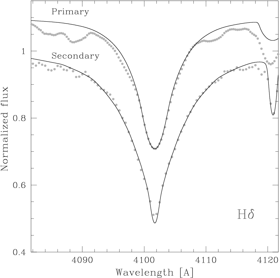
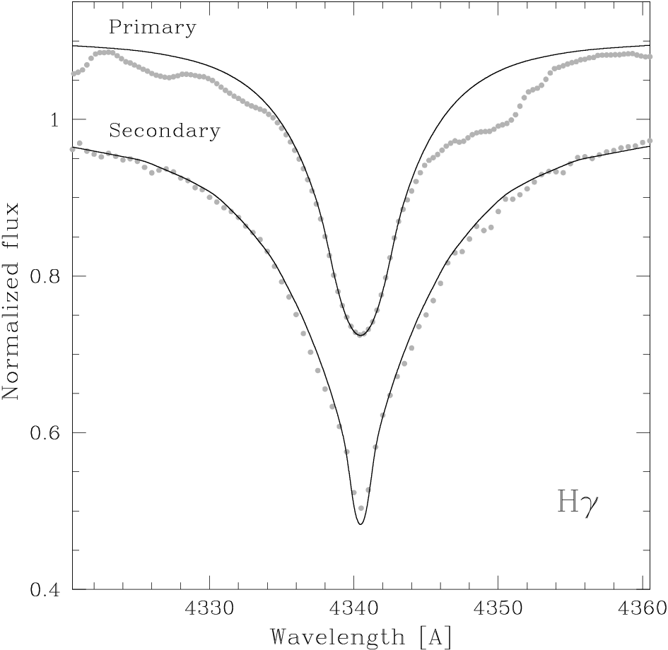
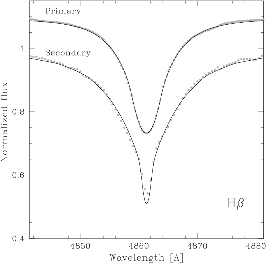
Before the spectra of individual binary components can be analysed to determine basic atmospheric parameters and individual abundances, they need to be renormalised to the individual continua of the component stars. This is done by means of the light ratio, which is often determined from photometric data for eclipsing binaries and by means of the constrained fitting (Tamajo et al., 2011, i.e., fitting for the light ratio simultaneously with other fundamental parameters,) for non-eclipsing systems. In the particular case of Spica, we fit for the light ratio and the other atmospheric parameters of the individual stellar components simultaneously, so that the light contribution of each of the stars is one of the output parameters from our spectrum analysis. The fundamental parameters and chemical composition of both stars were derived by fitting their disentangled spectra to a grid of synthetic spectra, based on the so-called hybrid approach. The latter assumes the usage of LTE-based atmosphere models and non-LTE spectral synthesis, in our case computed with the atlas9 (Kurucz, 1993), and detail (Butler, 1984) and surface (Giddings, 1981) codes, respectively. Justification of such approach is discussed in Nieva & Przybilla (2007). The adopted spectrum analysis procedure is discussed in Tkachenko et al. (2014a); Tkachenko et al. (2014b) in full detail but here we summarize a few key points only: 1) the whole analysis is based on the method of spectrum synthesis where a grid of synthetic spectra is fitted to the observations. Not only this concerns the determination of the atmospheric parameters of the individual stellar components but also their chemical compositions: both stars exhibit significant line broadening in their spectra, so the method of spectral synthesis is superior for the determination of individual abundances compared to the equivalent width measurements which suffers from heavy blending of spectral lines. 2) The determination of atmospheric parameters such as and , as well as the individual light factors is largely based on fitting the Balmer lines (Hδ, Hγ, and Hβ). 3) Microturbulent velocities are determined by fitting selected oxygen lines requiring a null correlation between the individual abundances and the equivalent widths of the corresponding spectral lines. The lines selected are those from Simón-Díaz (2010). We also use silicon lines as an additional check of the reliability of the determined microturbulent velocity. The projected rotational velocities of the stars are determined by fitting the metal line spectrum of each of the components.
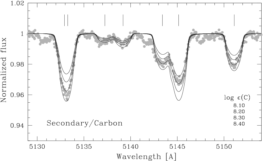
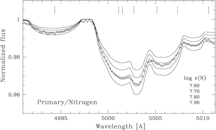
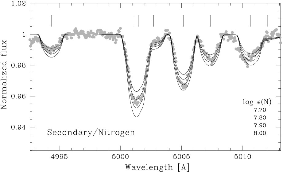
Tables 4 and 5 list the atmospheric parameters and individual abundances for both stellar components of the Spica binary system. The primary component is found to be hotter and more evolved than its companion, whereas both stars have the same chemical composition within the quoted error bars. The errors are 1 uncertainties, that for individual abundances take into account line-to-line scatter and the error propagation from the atmospheric parameters. The spectroscopically derived effective temperature of the secondary and surface gravities of both stars are in good agreement with the corresponding values of =20 585850 K, =3.750.11 dex, and =4.150.16 dex obtained from the light curve fitting and the dynamical masses and radii of the stars, respectively. The same concerns light factors: the light curve solution delivers contributions of 84.4/15.6% for the primary/secondary, which is in agreement with the spectroscopic findings within about 1%. Our atmospheric parameters are also in good agreement with the values reported by Lyubimkov et al. (1995), who found =24 700500/20 8001 500 K, =3.70.1/4.20.2 dex, and =1612/705 km s-1 for the primary/secondary component. Any discrepancies between our parameters and those determined by Lyubimkov et al. (1995) can be attributed to the fact that, in the latter study, the analysis was based on the original, composite spectra of the binary. The approach implemented in the current study and that is based on the analysis of the disentangled spectra of both components is more accurate as it does not suffer from spectral line blending due to the contribution of a companion star.
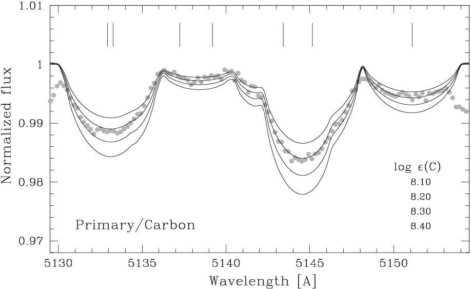
The quality of the fit to three Balmer lines (Hδ, Hγ, and Hβ) in the spectra of both stars is shown in Fig. 6. A set of carbon and nitrogen lines in the spectra of both binary components is illustrated in Fig. 7, along with the theoretical spectra computed assuming different abundances of these elements. A significant difference in rotational broadening of the spectral lines of the stars is easily caught by eye, as well as the similarity in their chemical compositions. Finally, we note that chemical compositions of both stars found in this study agree within the error bars with both the Cosmic Abundance Standard (Nieva & Przybilla, 2012) and chemical composition of the Sun as derived by Asplund et al. (2009). An exception is the abundances of carbon and aluminium in the atmosphere of the primary component, which seem to be slightly overabundant given our 1 uncertainties. We do not find any increase in the surface nitrogen abundance for either of the binary components, which puts both stars in the Group 1 of Hunter et al. (2008, Figure 1). For the further analysis, we will assume solar chemical composition for both binary components, as the above mentioned deviations of carbon and aluminium found for the primary will not have any impact on the analysis outlined in the next sections.
| Photometry | Spectroscopy | |||||||||||
| Pixel-by-pixel | RV | |||||||||||
| (magnitude) | (continuum units) | (km s-1) | ||||||||||
| fi | Freq (d-1) | Freq (Hz) | Amplitude | S/N | Freq (d-1) | Freq (Hz) | Amplitude | S/N | Freq (d-1) | Freq (Hz) | Amplitude | S/N |
| f1 | 0.694 | 8.030 | 0.00198(7) | 6.9 | 3.001 (12forb) | 34.722 | 0.014(1) | 10.8 | 2.998 (12forb) | 23.117 | 4.32(3) | 12.1 |
| f2 | 0.638 | 7.382 | 0.00114(7) | 5.5 | 5.748 | 66.504 | 0.012(2) | 7.4 | 5.751 | 66.539 | 1.93(3) | 4.5 |
| f3 | 1.486 | 17.193 | 0.00108(5) | 5.0 | 0.252 (forb) | 2.916 | 0.011(1) | 5.6 | 0.248 | 2.869 | 1.4 | 4.1 |
| f4 | 0.254 (forb) | 2.939 | 0.00083(5) | 4.4 | 2.162 | 25.014 | 0.007(1) | 4.0 | — | — | — | — |
| f5 | 0.741 (3forb) | 8.573 | 0.00082(5) | 4.1 | ||||||||
| f6 | 2.149 | 24.864 | 0.00063(4) | 4.0 | ||||||||
| f7 | 5.755 | 66.585 | 0.00057(3) | 5.5 | ||||||||
6 Frequency analysis and mode identification
In this section, we address the question of the variability intrinsic to either of the binary components, that manifests itself in terms of the brightness and line profile variations. The results of spectroscopic mode identification are also presented and discussed.
6.1 Previous work
The intrinsic variability of the primary component of Spica was extensively studied in the past. Shobbrook et al. (1969) were the first to report on the detection of light variations intrinsic to the evolved primary with frequency of 5.75 d-1 (66.53 Hz). The variability has been attributed to a radial pulsation mode, thus the star has been classified as a Cep-type variable. Smak (1970) came to the same conclusion and reported about a steady decrease of the dominant pulsation period at a rate of about 5 seconds per century. Shobbrook et al. (1972) investigated the system based on newly obtained photometric and spectroscopic data and confirmed the primary to be a variable star with the dominant frequency of 5.75 d-1 (66.53 Hz). However, the authors found the pulsation mode to be variable in amplitude with the variability being random. A second pulsation mode was detected at a frequency of 3.97 d-1 (45.93 Hz) in the radial velocity (RV) data and interpreted as the fundamental radial mode. The dominant mode was proposed to be due to the first overtone radial pulsation.
Walker et al. (1982) investigated new spectroscopic data obtained at orbital phases of large RV separation of the components. The authors detected “bumps” moving across line profiles of the primary, just in line with the expectations for non-radial pulsations.
A detailed study of the variability intrinsic to the primary component was performed by Smith (1985a); Smith (1985b). About 500 high resolution, high signal-to-noise-ratio (S/N) spectra were collected and analysed in the region of the Si III triplet at 4553, 4568, and 4575 Å. Clear, though low-amplitude, variability has been detected in the RV data of all three components of the triplet. The signal was found to be due to four modes, f3.68 d-1 (42.58 Hz), f7.5 d-1 (86.77 Hz), f0.49 d-1 (5.67 Hz), and f2.99 d-1 (34.59 Hz); no evidence of the previously reported radial mode with frequency of 5.75 d-1 (66.53 Hz) was found in the data. From the spacings between individual “bumps” detected in the silicon line profiles of the primary, the modes f1 and f2 were found to have geometries corresponding to and , respectively. The author also claims that these two modes have the same, high radial order n. The third mode at 0.49 d-1 (5.67 Hz) was attributed to the spectroscopic analog of the photometric ellipsoidal variability and identified as an mode. It is worth noting that this variability was detected indirectly, as a perturbing agent on the mode. Smith (1985a) concluded that the system has achieved angular momentum equilibrium by eventually rotating bisynchronously, i.e. with the rotation period of the primary being half of the orbital period of the binary.
The f2.99 d-1 (34.59 Hz) mode was analysed by Smith (1985b) in detail based on the data set obtained by Smith (1985a). The author found that the variability in question has very distinct behavior: unlike non-radial pulsations that show continuously travelling bumps from blue to red wing of the line profile or vice verse, this variability is characterized by nearly stationary absorption like features in the wings. The amplitude of these features was found to be variable, making them to disappear and reappear again during the variability cycle. Smith (1985b) found that the variability due to the f2.99 d-1 (34.59 Hz) mode can be well reproduced with a spherical harmonic function with the radial component of the displacement vector suppressed. Thus, the mode was found to have characteristics similar to those of toroidal modes, and was designated by the author as a “quasi-toroidal mode”.

Harrington et al. (2009) presented an analysis of high resolution spectra taken with the espadons instrument attached to the Canada France Hawaii Telescope. The authors reported the detection of the lines of the secondary component in their spectra, and classified both components as B-type stars. The authors found all weak spectral lines in their spectra to display discrete narrow features which could not be identified in He I and Balmer lines. The authors concluded that tidal flows exerted by the main-sequence secondary on the evolved primary are the main contributor to the short-term variability observed in the line profiles of the Spica system. Palate et al. (2013) arrived to a similar conclusion by analysing the data set obtained by Harrington et al. (2009) and using improved methodology. The conclusions of these two papers will be discussed in the context of our own results in the last section of the current study.
6.2 MOST photometry
The photometric solution obtained in Sect. 3 was used to compute residuals from the original MOST light curve illustrated in Fig. 1 (top panel). For the extraction of individual frequencies, amplitudes, and phases from the residual signal, we used the Lomb-Scargle version of the discrete Fourier transform (Lomb, 1976; Scargle, 1982) and consecutive prewhitening. A detailed mathematical description of the procedure can be found in Degroote et al. (2009).


The list of photometric frequencies extracted from the MOST light curve is given in Table 6 (first column, labeled “Photometry”). The frequencies with values of S/N above 4 are listed only. Those which are in common with the spectroscopic frequencies are highlighted in boldface. Frequencies f4 and f5 are linked to the orbital frequency of the binary system and are due to imperfect removal of the orbital signal from the original light curve. Frequency f7 has been previously reported in the literature as a radial pulsation mode with (randomly) variable amplitude (Shobbrook et al., 1969; Shobbrook et al., 1972, e.g.,). Smith (1985a) reported that this frequency could not be detected in his spectroscopic data, but stressed that there is no reason to assume that the mode will not return eventually. All other frequencies detected by us in the MOST photometry are new and have not been reported in the literature before. Based on the results of our spectroscopic investigations (see below), we conclude that it is the primary component that is responsible for the photometric variability occurring on top of the orbital signal.
6.3 High-resolution spectroscopy
Our very first exercise with the spectra was to figure out which of the stars is intrinsically variable in the system. To do so, we have selected all individual spectra in a narrow range of orbital phase to make sure that all dynamics we see in the line profiles is due to variability intrinsic to either of the binary components and not due to the orbital motion within the system. Also, if all variability was due to tides and/or tidally locked (Harrington et al., 2009; Palate et al., 2013, see, e.g.,), one would expect the signal to be repetitive with orbital cycle, i.e. nearly the same line profile pattern would be observed at a given orbital phase every orbital cycle (see Harrington et al., 2009, Figure 6). We did the above mentioned exercise for both quadratures, where the spectral features of the two stars are well separated in wavelength. Since the obtained results are essentially the same for both orbital phases, we illustrate only one of them in Fig. 8. The top panel shows the average Si III 4552.6 Å line, where the contribution of the secondary can be clearly distinguished from the one of the primary. The bottom panel illustrates a time-series of the residual profiles obtained by subtracting the average profile from the individual spectra. There are 162 spectra shown in total; all of them were used to compute the average profile shown in the top panel. One can clearly see bumps moving from blue to red wing of the profile of the primary component, the signal typical for non-radial pulsations. There is no variability in our data that could be attributed to the secondary component.
In the next step, we used the disentangled spectrum of the secondary obtained in Sect. 4 to subtract the contribution of this star from the composite spectra of the binary. To test how good the removal of the secondary’s contribution is, we did the frequency analysis of two different sets of the residual spectra: i) all 1731 spectra; ii) excluding the spectra where the lines of the secondary component merge with the lines of the primary. The goal of this exercise was to check which spurious frequencies will appear in the data due to the imperfect subtraction of the contribution of a companion star from the composite line profiles. We found that the frequencies at two and three times the orbital frequency (the second and the third harmonics of forb) show up in the first data set while they could not be detected in our second, orbital phase restricted data set. Thus, we conclude that these two frequencies are not real, and base our further analysis on the second set of 716 spectra. Interestingly, Smith (1985a) reported on the detection of 2forb periodicity in his spectra, and attributed it to an “equilibrium” tidal mode, which is basically a spectroscopic equivalent of the photometric ellipsoidal variability. This type of signal was also theoretically predicted by Harrington et al. (2009) to occur in the Spica system due to the tidal flows exerted by the components on each other. Our test with the real data shows that the signal at low order harmonics of the orbital frequency is easily introduced into the data artificially, when the contribution of the secondary component is taken into account inappropriately, one way or the other.
The individual frequencies have been extracted from both RVs (computed as the first order moment of the spectral line) and the line profiles themselves, using discrete Fourier-transform (DFT) and a consecutive prewhitening procedure as implemented in the famias (Zima, 2008) software package. Following the procedure described in Tkachenko et al. (2014a), the DFT was computed up to the Nyquist frequency, the amplitudes and phases were optimised at each step of the prewhitening procedure while keeping the frequency values fixed, and the frequencies were accepted as significant ones if their S/N was higher or equal to 4 (Breger et al., 1993). For the analysis, we used the Si III triplet 4553, 4568, and 4575 Å, but neglected all other lines potentially sensitive to non-radial pulsations (like He or Mg lines), because of high degree of their blending due to the rapid rotation of the star. The final list of frequencies is given in the second column of Table 6, labeled “Spectroscopy”. Frequencies f5.75 d-1 (66.53 Hz) and f0.25 d-1 (2.89 Hz) were found both in the RVs and in the line profiles themselves, and agree within the error bars with the frequencies f7 and f4 detected in the photometric data. As it has been discussed in the previous section already, the former is likely a radial mode whereas the latter is the orbital frequency. There is a frequency, f3.00 d-1 (34.71 Hz), that shows up in both spectroscopic observables, but could not be detected in the MOST photometry. This one is close to the 12th harmonic of the orbital frequency and is thus a good candidate for a mode excited by means of the dynamical tides expected to occur in eccentric binary systems. The same frequency was detected by Smith (1985a) in his spectroscopic data and explained in terms of a tidally forced “quasi-toroidal” mode (Smith, 1985b). The last frequency, f2.16 d-1 (24.99 Hz), could be detected in the line profiles but not in the RV data, and has a low amplitude both in the spectroscopic and the photometric data.
We used famias to identify all three modes, f1, f2, and f4, detected in our spectroscopic data. For that, we used the Fourier-parameter fit method (Zima et al., 2006, FPF,), which is best suitable for mode identification in rapidly rotating stars. Identification of pulsation modes requires a knowledge of fundamental stellar parameters like mass, radius, effective temperature, surface gravity, etc. These were set to the values obtained from our combined photometric and spectroscopic solution, as summarized in the third column of Table 7. The individual masses and radii of the stars were computed from binary dynamics and we refer the reader to Tkachenko et al. (2014b, Section 5) for any details. The luminosities were computed from the dynamical radii and effective temperatures of stars. In the first step, the modes were identified independently of each other, that is each time the star was treated as a mono-periodic pulsator. This often allows to narrow the range in free parameters, particularly in and quantum numbers, which in turn significantly reduces the calculation time when the multi-periodic solution is searched for. To provide sufficient spatial resolution, we divided the stellar surface into 10 000 segments. At each iteration step the amplitude and phase distributions across the profile were optimized along with the zero-point profile. Besides the and quantum numbers and intrinsic amplitudes of the modes, the intrinsic width of the Gaussian profile , projected rotational velocity of the star , and the inclination of its rotational axis were set as free parameters. Since famias assumes an alignment between rotation and pulsation axes, it is possible to check for possible spin-orbit misalignment by keeping as a free parameter. Figure 9 illustrates the distributions of amplitude and phase across the line profile for all three modes: f3.001 d-1 (top left), f5.748 d-1 (top right), and f2.162 d-1 (bottom). The best fit models with values below 20 are overplotted with the lines of different style; the corresponding mode geometries are indicated in the plots. Such large values of , that are obviously linked to the inconsistency between the model and observations in Fig. 9, can be attributed to the fact the high-order rotation effects are not taken into account in the famias model. The f3.001 d-1 (34.722 Hz) mode is unambiguously identified as an mode. No unique solution could be found for the modes f2 and f4, though the range in both quantum numbers is well constrained: we find that the former mode is likely a radial or mode, while the latter is either or mode. All our best solutions with values below 20 suggest a range in the inclination angle of rotation axis between 53 and 66 degrees. This value is in good agreement with the orbital inclination of degrees.
| Parameter | Unit | Primary | Secondary | ||
|---|---|---|---|---|---|
| Mass, | M⊙ | 11.43 | 1.15 | 7.21 | 0.75 |
| Radius, | R⊙ | 7.47 | 0.54 | 3.74 | 0.53 |
| Luminosity, | L⊙ | 4.312 | 0.095 | 3.353 | 0.181 |
| Effective temperature1, | K | 25 300 | 500 | 20 900 | 800 |
| Surface gravity1, | dex | 3.71 | 0.10 | 4.15 | 0.15 |
| 1 adopted from spectroscopy (see Table 4) | |||||
7 Evolutionary models
The mesa stellar structure and evolution code (Paxton et al., 2011; Paxton et al., 2013) was used to compute evolutionary models for both components of the Spica system. Given that the secondary component rotates at about 10% of its critical velocity, we have chosen to compute non-rotating models for this star. Contrary, the primary is found to rotate at 30% of its break-up velocity, and thus the rotation could not be neglected in the evolutionary model calculations for this binary component. The initial abundance fractions (X, Y, Z) = (0.710, 0.276, 0.014) are those from Nieva & Przybilla (2012), in agreement with the spectroscopic findings (cf. Sect. 5). Convective core overshoot is described with an exponentially decaying prescription of Herwig (2000). The Ledoux criterion is used in the convection treatment. The OPAL opacity tables Iglesias & Rogers (1996) and MESA equation-of-state are used.
Figure 10 illustrates the position of both stellar components of the Spica system in the - diagram. The error bars are those obtained from 1 combined spectroscopic and photometric uncertainties (cf. Table 4). The evolutionary tracks are shown with solid lines for dynamical masses of both stars and the corresponding error bars (cf. Table 7). The tracks were computed for the overshoot parameter ( Hp); we also show the track computed with ( Hp) for a single mass value to illustrate the effect of overshoot on the evolutionary path of the star. Dashed lines show isochrones corresponding to 11.5 (bottom), 12.5 (middle), and 13.5 (top) Myr. The latter were computed assuming overshoot of . We find that the position of the unevolved secondary agrees very well with its dynamical mass evolutionary track. The same holds for the primary when the error bars on the mass, , and of the star are taken into account. The positions of both stars are in good agreement with the isochrone corresponding to 12.5 Myr. By taking into account the errors on and for the primary component, we estimate the accuracy for the age to be of Myr.
8 Summary and Discussion

In this paper, we presented a detailed analysis of the Spica close binary system, based on high-resolution spectroscopy obtained with the coralie spectrograph and space-based photometry gathered with the MOST mission. In total, 1731 spectra and 23 days of nearly continuous photometric measurements have been analysed with the state-of-the-art modelling techniques. We found that the Spica system is close to showing a grazing secondary eclipse, the fact exciting by itself but hardly helpful for the analysis in terms of a better precision on the fundamental parameters of the component stars. Both binary components are found to have similar chemical composition consistent with the cosmic abundances derived from Galactic OB stars (Nieva & Przybilla, 2012).
A comparison of the positions of both stars in the - diagram with the mesa evolutionary models reveals a good agreement for the secondary component. This result differs from the one obtained by us for the V380 Cyg (Tkachenko et al., 2014a) and Sigma Scorpii (Tkachenko et al., 2014b) systems, where the unevolved secondary components were found to show significant discrepancy between their evolutionary and dynamical masses. A small mass discrepancy is not excluded for the primary component of Spica, though no definite conclusion can be drawn on this aspect because of rather large uncertainty of about 10% in the stellar mass.
Contrary to Harrington et al. (2009) and Palate et al. (2013) suggesting that the line profile variations observed in the primary component can be naturally explained in terms of surface tidal flows exerted on it by the secondary, we find a clear evidence of non-radial pulsation modes in the system. One of the modes is interpreted by us as being excited through a resonance between the free oscillation of the primary and the dynamical tides in the binary system. If confirmed with future observations, the Spica system will be the first massive binary (with the mass of the pulsating component larger than 5 M⊙) in which tidally-induced pulsations have been detected. Unfortunately, our attempt to carry out detailed asteroseismic modelling for the primary component of the Spica system was unsuccessful due to insufficient frequency resolution achieved with our data. In the result, several tens of models with values below 1 were found when attempting to fit the observed frequencies, implying that the actual errors on individual frequencies are larger than the difference between the observed and theoretical values. The corresponding models cover entire parameter range in the fundamental stellar parameters such as the effective temperature, surface gravity, mass, radius, etc., implying that detailed asteroseismic analysis is not feasible with the data set we currently have. An accumulation of additional spectroscopic material would help to increase the frequency resolution, and thus would make the seismic analysis feasible for the primary component of Spica.
The mass discrepancy problem remains an unresolved issue in the massive binary research area for at least a few decades. It clearly points to some shortcomings in the current theories of stellar structure and evolution since the masses of the component stars measured from binary dynamics are model-independent values. As of today, the mass discrepancy problem, one way or the other, was addressed in several studies (Burkholder et al., 1997; Pavlovski et al., 2009; Tkachenko et al., 2014a; Tkachenko et al., 2014b; Garcia et al., 2014, e.g.,). The majority of the studies reported on a significant discrepancy between the dynamical and evolutionary masses, in a very few cases, the models were successful in matching the dynamical masses of the component stars. Revealing the shortcomings in the current theories of stellar structure and evolution requires a statistically significant, homogeneously analysed sample of massive binaries, whereas currently the analysis methods as well as the evolutionary models used by different authors are quite diverse. Spica is the third massive binary system, after V380 Cyg and Sco, that has been analysed by us in a consistent, homogeneous way, using the same modelling tools as for the other two binaries. We will extend our sample of massive binaries by adding about a dozen of eclipsing systems that we have recently discovered in the Campaign 0 data of the K2 mission. More systems are expected to be found in other fields of view of the K2 missions as well. With a few dozens of the systems in total analysed in a consistent way, we will be able to get more insight into the nature of the mass discrepancy problem for massive stars.
acknowledgements
The research leading to these results has received funding from the European Community’s Seventh Framework Programme FP7-SPACE-2011-1, project number 312844 (SPACEINN), and from the Fund for Scientific Research of Flanders (FWO), Belgium, under grant agreement G.0B69.13. E.M. has received funding from the People Programme (Marie Curie Actions) of the European Unions Seventh Framework Programme FP7/2007-2013/ under REA grant agreement n∘623303 for the project ASAMBA. K.P. was (partially) supported by the Croatian Science Foundation under the grant 2014-09-8656. K.Z. acknowledges support by the Austrian Fonds zur Foerderung der wissenschaftlichen Forschung (FWF, project V431-NBL). Mode identification results with the software package famias developed in the framework of the FP6 European Coordination Action HELAS (http://www.helas-eu.org/). A.T. dedicates this work to his grandfather, A. Solomchenko, who passed away in January 2016.
References
- Aerts et al. (1992) Aerts, C., de Pauw, M., & Waelkens, C. 1992, A&A, 266, 294
- Aerts et al. (2010) Aerts, C., Christensen-Dalsgaard, J., & Kurtz, D. W. 2010, Asteroseismology, Springer, Heidelberg
- Asplund et al. (2009) Asplund, M., Grevesse, N., Sauval, A.J., & Scott, P., 2009, ARA&A, 47, 481
- Aufdenberg et al. (2007) Aufdenberg, J. P., Ireland, M. J., Mérand, A., et al. 2007, IAU Symposium, 240, 271
- Breger et al. (1993) Breger, M., Stich, J., Garrido, R., et al. 1993, A&A, 271, 482
- Brott et al. (2011) Brott, I., Evans, C. J., Hunter, I., et al. 2011, A&A, 530, A116
- Burkholder et al. (1997) Burkholder, V., Massey, P., & Morrell, N. 1997, ApJ, 490, 328
- Butler (1984) Butler, K. 1984, PhD thesis, University of London, UK
- Claret (2000) Claret, A. 2000, A&A, 363, 1081
- Degroote et al. (2009) Degroote, P., Aerts, C., Ollivier, M., et al. 2009, A&A, 506, 471
- Degroote et al. (2013) Degroote, P., Conroy, K., Hambleton, K., et al. 2013, EAS Publications Series, 64, 277
- Desmet et al. (2009) Desmet, M., Aerts, C., Matthews, J. M., et al. 2009, American Institute of Physics Conference Series, 1170, 376
- Garcia et al. (2014) Garcia, E. V., Stassun, K. G., Pavlovski, K., et al. 2014, AJ, 148, 39
- Giddings (1981) Giddings, J. R. 1981, PhD thesis, University of London, UK
- Hadrava (1995) Hadrava, P. 1995, A&AS, 114, 393
- Hambleton et al. (2013) Hambleton, K. M., Kurtz, D. W., Prša, A., et al. 2013, MNRAS, 434, 925
- Harrington et al. (2009) Harrington, D., Koenigsberger, G., Moreno, E., & Kuhn, J. 2009, ApJ, 704, 813
- Herbison-Evans et al. (1971) Herbison-Evans, D., Hanbury Brown, R., Davis, J., & Allen, L. R. 1971, MNRAS, 151, 161
- Herrero et al. (1992) Herrero, A., Kudritzki, R. P., Vilchez, J. M., et al. 1992, A&A, 261, 209
- Herwig (2000) Herwig, F. 2000, A&A, 360, 952
- Hunter et al. (2008) Hunter, I., Brott, I., Lennon, D. J., et al. 2008, ApJL, 676, L29
- Iglesias & Rogers (1996) Iglesias, C. A. & Rogers, F. J. 1996, ApJ, 464, 943
- Ilijic et al. (2004) Ilijic, S., Hensberge, H., Pavlovski, K., & Freyhammer, L. M. 2004, Spectroscopically and Spatially Resolving the Components of the Close Binary Stars, 318, 111
- Kudritzki (1980) Kudritzki, R.-P. 1980, A&A, 85, 174
- Kurucz (1993) Kurucz, R. 1993, ATLAS9 Stellar Atmosphere Programs and 2 km/s grid. Kurucz CD-ROM No. 13. Cambridge, Mass.: Smithsonian Astrophysical Observatory, 1993., 13
- Lomb (1976) Lomb, N. R. 1976, Ap&SS, 39, 447
- Lyubimkov et al. (1995) Lyubimkov, L. S., Rachkovskaya, T. M., Rostopchin, S. I., & Tarasov, A. E. 1995, Astronomy Reports, 39, 186
- Nieva & Przybilla (2007) Nieva, M. F., & Przybilla, N. 2007, A&A, 467, 295
- Nieva & Przybilla (2012) Nieva, M.-F., & Przybilla, N. 2012, A&A, 539, A143
- North et al. (2007) North, J. R., Davis, J., Tuthill, P. G., Tango, W. J., & Robertson, J. G. 2007, MNRAS, 380, 1276
- Palate et al. (2013) Palate, M., Koenigsberger, G., Rauw, G., Harrington, D., & Moreno, E. 2013, A&A, 556, A49
- Pápics et al. (2012) Pápics, P. I., Briquet, M., Baglin, A., et al. 2012, A&A, 542, A55
- Pápics et al. (2013) Pápics, P. I., Tkachenko, A., Aerts, C., et al. 2013, A&A, 553, A127
- Pavlovski & Hensberge (2005) Pavlovski, K., & Hensberge, H. 2005, A&A, 439, 309
- Pavlovski & Southworth (2009) Pavlovski, K., & Southworth, J. 2009, MNRAS, 394, 1519
- Pavlovski et al. (2009) Pavlovski, K., Tamajo, E., Koubský, P., et al. 2009, MNRAS, 400, 791
- Paxton et al. (2011) Paxton, B., Bildsten, L., Dotter, A., Herwig, F., Lesaffre, P., & Timmes, F. 2011, ApJS, 192, 3
- Paxton et al. (2013) Paxton, B., Cantiello, M., Arras, P., et al. 2013, ApJS, 208, 4
- Prša & Zwitter (2005) Prša, A., & Zwitter, T. 2005, ApJ, 628, 426
- Prša et al. (2013) Prša, A., Degroote, P., Conroy, K., et al. 2013, EAS Publications Series, 64, 259
- Scargle (1982) Scargle, J. D. 1982, ApJ, 263, 835
- Shobbrook et al. (1969) Shobbrook, R. R., Herbison-Evans, D., Johnston, I. D., & Lomb, N. R. 1969, MNRAS, 145, 131
- Shobbrook et al. (1972) Shobbrook, R. R., Lomb, N. R., & Herbison-Evans, D. 1972, MNRAS, 156, 165
- Simón-Díaz (2010) Simón-Díaz, S. 2010, A&A, 510, A22
- Simon & Sturm (1994) Simon, K. P., & Sturm, E. 1994, A&A, 281, 286
- Smak (1970) Smak, J. 1970, AcA, 20, 75
- Smith (1985a) Smith, M. A. 1985a, ApJ, 297, 206
- Smith (1985b) Smith, M. A. 1985b, ApJ, 297, 224
- Tamajo et al. (2011) Tamajo, E., Pavlovski, K., & Southworth, J. 2011, A&A, 526, A76
- Thompson et al. (2012) Thompson, S. E., Everett, M., Mullally, F., et al. 2012, ApJ, 753, 86
- Tkachenko et al. (2009) Tkachenko, A., Lehmann, H., & Mkrtichian, D. E. 2009, A&A, 504, 991
- Tkachenko et al. (2010) Tkachenko, A., Lehmann, H., & Mkrtichian, D. 2010, AJ, 139, 1327
- Tkachenko et al. (2014a) Tkachenko, A., Degroote, P., Aerts, C., et al. 2014a, MNRAS, 438, 3093
- Tkachenko et al. (2014b) Tkachenko, A., Aerts, C., Pavlovski, K., et al. 2014b, MNRAS, 442, 616
- Vogel (1890) Vogel, H. C. 1890, The Observatory, 13, 367
- Walker et al. (1982) Walker, G. A. H., Moyles, K., Yang, S., & Fahlman, G. G. 1982, PASP, 94, 143
- Walker et al. (2003) Walker, G., Matthews, J., Kuschnig, R., et al. 2003, PASP, 115, 1023
- Welsh et al. (2011) Welsh, W. F., Orosz, J. A., Aerts, C., et al. 2011, ApJS, 197, 4
- Wilson (1979) Wilson, R. E. 1979, ApJ, 234, 1054
- Wilson & Devinney (1971) Wilson, R. E., & Devinney, E. J. 1971, ApJ, 166, 605
- Zima (2008) Zima, W. 2008, Communications in Asteroseismology, 155, 17
- Zima et al. (2006) Zima, W., Wright, D., Bentley, J., et al. 2006, A&A, 455, 235