Stochastic Rotation Dynamics simulations of wetting multi–phase flows

Particle based simulation methods obtain the collective dynamics of the fluid phases from the motion of a large number $N$ of point particles $i$ of mass $m$ that can adopt continuous positions, $\mathbf{x}_{i}$, and velocities, $\mathbf{v}_{i}$, in three dimensional Euclidean space. The dynamics of the particles consist of a sequence of streaming and collision steps. During free streaming, particles move deterministically between time $t$ and $t+\Delta t$. New positions $\mathbf{x}_{i}(t+\Delta t)$ and velocities $\mathbf{v}^{\prime}_{i}(t+\Delta t)$ at the end of the streaming step are consequently given by

and

respectively, where a constant external force $\mathbf{f}_{\rm ex}$ acting on all particles is included. In our notation all pre–collisional quantities that may change during collision are marked with a prime. The corresponding post–collisional quantities (at the beginning of the next streaming step) are not primed.

In order to introduce an interaction among particles, i.e. an exchange of linear momentum, the particles are sorted into collision cells $\xi$ after each streaming step. In the present algorithm we use a cubic grid of uniform spacing $a$ where the number of particles per cell, $N_{\xi}$, fluctuates around an average value $\left\langle N_{\xi}\right\rangle$.

In every collision, which occurs instantaneously at time $t+\Delta t$ the velocities of the particles are decomposed into the center of mass velocity $\mathbf{u}_{\xi}$ of all particles belonging to cell $\xi$ and a remaining, fluctuational part $\widetilde{\mathbf{v}}_{i}^{\prime}=\mathbf{v}^{\prime}_{i}-\mathbf{u}_{\xi}$. In all variants of SRD, linear momentum between particles in a cell is exchanged through a rotation of the fluctuational velocity components. The particle velocity after the effective collision step is

where $\boldsymbol{\Omega}_{\xi}$ denotes a rotation around an axis $\mathbf{R}_{\xi}$ by an angle $\alpha$. In order to achieve molecular chaos, the unit vector $\mathbf{R}_{\xi}$ is randomly drawn from the surface of the three dimensional unit sphere for every cell $\xi$ and in every collision step. Most implementations of the mono–phase SRD algorithm employ a fixed rotation angle $\alpha$. Density correlations of the fluid particles which may occur for small mean free paths $\lambda_{\rm MFP}=\Delta t\sqrt{k_{B}T/m}\ll a$ are avoided through a shift of the collision grid before each collision step. The Cartesian components of the random shift $\boldsymbol{\zeta}$ are drawn uniformly from the interval $[-a/2,a/2]$ [46].

As the particle collisions in standard SRD obey conservation of mass, linear momentum and energy we observe both diffusive and advective transport of the conserved quantities on length scales larger than the grid spacing $a$. The evolution of spatial and temporal averages of hydrodynamic quantities like velocity $\mathbf{u}$ and mass density $\rho=nm$, with the number density $n=N_{\xi}/V_{\xi}$ in the SRD fluid conform to a continuum description by the Navier–Stokes equation [15]. It was shown that the detailed balance condition for the SRD collisions is satisfied and that therefore an H theorem exists [15, 47, 48]. The equation of state of a SRD fluid is identical to the equation of state of an ideal gas. However, recently it was shown that SRD fluids exhibit a nonzero bulk viscosity which seems to contradict the ideal gas assumption [65]. As the bulk viscosity is determined by the particle collisions the ideal gas limit is reached for large collision time steps. This means a collisional dominated system (short mean free path $\lambda_{\rm MFP}$, non–zero bulk viscosity) is more liquid–like whereas a kinetic dominated system (large mean free path $\lambda_{\rm MFP}$, vanishing bulk viscosity) is more gas–like [65].

Several authors derived explicit expressions for the transport coefficients for a mono–phase SRD fluid based on the Green–Kubo formalism  [47, 48, 53, 56]. Alternatively to this equilibrium approach the transport coefficients can also be measured out of equilibrium, like e.g. in shear flow. This was first shown in Ref. [46] and later extended in Refs. [66, 57]. For a comprehensive summary, we refer to the overview given in Ref. [18] and the references therein.

In general, SRD fluids are Newtonian with a kinematic viscosity in three dimensions as given by e.g. [53, 56]

where $\eta$ denotes the dynamic viscosity and $k_{B}T$ is the thermal energy scale.

When solid walls are introduced in a SRD system the fluid dynamic boundary conditions need to be considered. In order to guarantee a no–slip boundary condition for the average fluid velocities, a generalization of the bounce–back rule for partially filled cells is employed [67]. In the naïve formulation of the bounce–back rule, particles travel back into the direction of their incidence after having collided with the solid boundaries during free streaming. Because the position of the solid boundaries relative to the coarse–graining grid changes between every inter–particle collision step due to the random grid shift, it is necessary to add a virtual phase resting inside the walls to match the bulk particle density in the underfilled cells. These virtual wall–particles participate in the collisions and are generated before and removed after every inter–particle collision step, and guarantee a no–slip boundary condition at the walls [67]. If, however, partial slip is desired at the solid walls it is possible to tune the local particle density inside the walls [64] or choose an alternate reflection mechanism [63] and vary therewith the local slip length. Note, that in general the method of virtual particles is only needed for systems where the viscosity is dominated by the collisional contribution e.g. short mean free paths $\lambda_{\rm MFP}$. When the mean free path is larger than $\lambda_{\rm MFP}\gtrsim 0.6\>a$ and ergo the viscosity is dominated by the kinetic contribution, the no–slip boundary condition is readily achieved provided that the bounce–back rule is applied [68].

Unless explicitly defined we set grid size $a$, collisional time step $\Delta t$, particle mass $m$ and the Boltzmann constant $k_{B}$ to unity. If these rescaled units are used, the mean free path of the particles $\lambda_{\rm MFP}$ depends only on temperature $T$.

In their basic formulation MPC/SRD algorithms do not conserve angular momentum [15, 24, 43] but can be easily extended to do so [59]. Generally, when a mono–phase system is considered, the lack of angular momentum conservation only modifies the viscosity of the fluid [24]. However, following Ref. [24] there are several cases where angular momentum conservation is essential:

1. 1.

   the boundary conditions on walls are given by forces including torques (circular Couette flow)

2. 2.

   finite–sized objects that rotate in fluids by hydrodynamic stress (colloidal and polymer suspensions)

3. 3.

   fluids with different viscosities are in contact.

Especially the last point becomes important when studying multi–phase or microfluidic systems where the fluids involved often have a certain viscosity contrast. Thus, we like to point out that especially in $\rm{SRD}^{mc}$ vorticity is a hydrodynamical degree of freedom that needs to be locally conserved during collisions. Because in standard SRD implementations angular momentum conservation depends on the predefined collision angle $\alpha$ another approach has to be used in $\rm{SRD}^{mc}$ where the collision angle $\alpha$ is calculated individually for every collision cell. We employ a straight forward protocol where the angular momentum in every collision cell is first calculated and then subtracted from the individual particle velocities before the actual collision. This procedure ensures that the fluctuational velocities subject to the collision operator are effectively irrotational.

To enforce local conservation of angular momentum the following steps are introduced into the collision operation from eqn. (3) at time $t+\Delta t$. The total angular momentum of a collision cell $\mathbf{L}^{\prime}_{\xi}$ is calculated by

where $\widetilde{\mathbf{x}}_{i}$ is the relative position of particle $i$ to the center of mass of the collision cell $\xi$. Additionally the moment of inertia tensor $\mathbf{I}_{\xi}$ is calculated by

with $\mathbf{r}_{i}$ the vector pointing from the center of mass to particle $i$ and $\delta_{\alpha\beta}$ the Kronecker symbol. Then the vorticity $\boldsymbol{\omega}^{\prime}_{\xi}$ is given by

which is twice the angular velocity. The contribution of the angular momentum of the cell on particle $i$ is then calculated by

Consequently, when considering the velocity from eqn. (8) the actual relative velocity of particle $i$ is

so that the fluctuational velocities $\widetilde{\mathbf{v}}^{\prime}_{i}$ in a collision cell are irrotational. The fluctuational velocities $\widetilde{\mathbf{v}}^{\prime}_{i}$ from eqn. (9) are then subjected to the standard SRD collision. As the collision operator itself generates angular momentum on the post–collisional fluctuational velocities $\widetilde{\mathbf{v}}_{i}$ this additional vorticity needs to be removed. Therefore, the post–collisional angular momentum $\mathbf{L}_{\xi}$, vorticity $\boldsymbol{\omega}_{\xi}$ and the correction to the fluctuational velocity $\widehat{\mathbf{v}}_{i}$ are calculated similar to eqns. (5, 7, 8) by

and

After the collision procedure the new particle velocities are

where the contribution from the collision operator $\widehat{\mathbf{v}}_{i}$ to the angular momentum is removed and the pre–collisional contribution $\widehat{\mathbf{v}}^{\prime}_{i}$ is added back. In this way the pre–collisional angular momentum $\mathbf{L}^{\prime}_{\xi}$ is restored. The method employed here effectively conserves angular momentum with an additional computational overhead of $\approx 20\%$ tested up to a total amount of $10^{7}$ particles per system. This increase in computational time is comparable to values reported for angular momentum conserving MPC methods with Anderson thermostat (MPC–AT$+\alpha$) [18]. In the course of this work we will distinguish between the angular momentum conserving ($\rm{SRD}^{mc}_{+}$) and not conserving ($\rm{SRD}^{mc}_{-}$) case, respectively.

In any non–equilibrium MPC/SRD simulation with external driving of the particles the control of the system temperature is essential. Injection of work into the MPC/SRD fluid and dissipation through viscous heating may occur through external forces or by imposed motion of the walls confining the particles. A standard method to enforce a constant temperature in a MPC fluid is to implement an Anderson thermostat (MPC–AT) [28, 24, 69]. Instead of rotating the relative velocities in a collision cell, new relative velocities are generated at each time step from a Maxwell Boltzmann distribution with zero mean and temperature dependent standard deviation. Obviously, an Anderson thermostat is not applicable to SRD based algorithms because during collisions relative velocities are rotated rather than newly generated.

In continuation with the standard SRD method and due to its simplicity in implementation we use a profile–unbiased local thermostat (PUT) in this work. This ensures control of the thermal fluctuations while keeping unaffected the macroscopic velocity field [70, 69, 61]. In a recent study PUT was compared to a Maxwell–Boltzmann scaling (MBS) method as introduced in Ref. [61] and in regard to the measured fluid viscosities was found to perform equally well [71]. The fluctuational velocities of each cell $\xi$ are rescaled after each collision step as $\widetilde{\mathbf{v}}_{i}\rightarrow\lambda_{\xi}\widetilde{\mathbf{v}}_{i}$, where the correction factor is calculated by

The term $3(N_{\xi}-X)$ accounts for the particles spatial degrees of freedom (DOF) in three dimensions minus the DOF of the center of mass of the collision cell. If angular momentum is not conserved then $X=1$ (only translational DOF). In case of angular momentum conservation $X=2$ (translational and rotational DOF) and $\widetilde{\mathbf{v}}_{i}$ in eqn. (14) has to be replaced by $\widetilde{\mathbf{v}}_{i}-\widehat{\mathbf{v}}_{i}$ to account for the additional rotational components.

The $\rm{SRD}^{mc}$ algorithm of Inoue et al. [1] utilizes a modified collision operator that actively creates a repulsive interaction between different particles species, but still allows for a diffusive momentum exchange between particles in the homogeneous phases. Different particle species (phases) are introduced through colors $c=1,\dots,N_{p}$ assigned to each individual particle. At each collision step the color flux

is computed while color–gradients $\boldsymbol{\nabla}n_{c}(\xi)$ are estimated for each color $c$ in each cell $\xi$ from the number of particles of the same color in the next–nearest neighboring cells. Then, after selecting a random rotation axis $\mathbf{R}_{\xi}$ in each cell, the rotation angle $\alpha_{\xi}$ is constructed such that, the color action

in cell $\xi$ is maximized. The symmetric interaction matrix $\kappa_{c\,c^{\prime}}$ weights the relative tendency of colored particles to repel or attract each other. The necessary condition for a maximum

has two solutions $\alpha_{\xi}^{\rm+}$ and $\alpha_{\xi}^{\rm-}$ in $[-\pi,\pi]$. Given the color gradients and the color fluxes the rotation angle $\alpha_{\xi}$ that satisfies condition eqn. (17) can be computed from expression

employing the weighted color gradient

is used. In order to guarantee that the color action is in a maximum after the rotation the actual rotation (collision) angle $\alpha_{\xi}$ must be chosen from the two solutions of eqn. (18) according to the condition

Phase segregation between particle species $c\neq c^{\prime}$ is achieved by a negative sign $\kappa_{c\,c^{\prime}}<0$, as the particles of color $c$ are forced to move to regions where the concentration of particles with color $c^{\prime}$ is low. The opposite sign $\kappa_{c\,c^{\prime}}>0$ leads to mixing of particles of color $c$ and $c^{\prime}$. Diagonal entries are set to unity.

In its most fundamental definition, stress is a flux of linear momentum and is described in three dimensions by a tensor $\boldsymbol{\sigma}$ of rank two with nine independent components. Transport of linear momentum in a fluid proceeds either through collective motion of particles during streaming or by exchange of linear momentum between particles during collisions. Referring to these two modes of momentum transport the total stress $\boldsymbol{\sigma}$ can be split into a kinetic contribution $\boldsymbol{\sigma}^{\mathrm{(kin)}}$ and a collisional contribution $\boldsymbol{\sigma}^{\mathrm{(col)}}$, so that

holds. Despite its definition as a flux of momentum, stress is measured in most particle based simulations by volume averaging of suitable expressions of particle positions and velocities. Global averages of the stress tensor in the absence of external forces can be obtained from the virial theorem (see e.g. [72, 73]). In Cartesian components the stress average then reads

where $V$ is the volume of the simulation domain, $N$ is the total number of particles in the system and $\mathbf{r}$ is the position of particle $i$ inside the system, respectively. Angular brackets $\langle\dots\rangle$ indicate time averages of the enclosed variable(s). The first term in eqn. (22) refers to the kinetic contribution $\boldsymbol{\sigma}^{\mathrm{(kin)}}$ whereas the second term refers to the collisional contribution $\boldsymbol{\sigma}^{\mathrm{(col)}}$, respectively. Expressions analogous to eqn. (22) have been used before to measure the stress tensor in mono–phase MPC/SRD fluids [66, 59, 60].

The definition of stress as momentum flux provides an alternative approach to volume averaging methods. In the following part we describe the measurement of the stress tensor by area–weighted averages as outlined e.g. for systems with many–body interactions by Refs. [74, 75]. In this way global and local contributions to the stress tensor can be determined. To compute the local flux of linear momentum in the $\rm{SRD}^{mc}$ fluid, the simulation domain is subdivided by control planes crossing the system in all three dimensions. In particular, we consider three stacks of planes normal to the direction of the three unit vectors $\mathbf{e}_{x}$, $\mathbf{e}_{y}$, and $\mathbf{e}_{z}$ of the Cartesian coordinate system. The control planes partition the simulation box into small cubes. The distance $d$ between every pair of neighboring planes is uniform and equals a certain fraction of the size of the collision grid $a$. Each stress plane is tiled into an array of small squares $\mathcal{A}$ with the lateral dimensions $d$. Each small square $\mathcal{A}$ is oriented normal to $\mathbf{e}_{\alpha}$ and centered around the intersection points $\mathbf{x}_{A}$ of the three squares $\mathcal{A}(\mathbf{x}_{A},\alpha)$ into the three directions $\mathbf{e}_{\alpha}$ with $\alpha\in\{x,y,z\}$. All stress components measured in the $\rm{SRD}^{mc}$ simulations are collocated at the intersection points $\mathbf{x}_{A}$.

Figure 1 illustrates the stress measurement in our $\rm{SRD}^{mc}$ simulations. Panel (a) shows a small fraction of a three–dimensional system that is subdivided by three control planes for each spatial dimension and therewith forming a regular lattice of points $\mathbf{x}_{A}$ with corresponding small control surfaces $\mathcal{A}$ (red planes). In the example shown in Fig. 1, we chose the resolution of the stress grid to be two times larger than the grid size $a$ so that the distance between the individual stress planes is $d=a/2$ and, hence, the area of a single sub–plane in three dimensions is $A_{\mathcal{A}}=d^{2}=a^{2}/4$. As an example, panel (b) shows the magnified region around a single point $\mathbf{x}_{A}$. In panels (c) and (d) the measurement of the kinetic and collisional contribution is exemplified.

During streaming (Fig. 1c) particles move from the pre–streaming (blue) to the post–streaming position (black), respectively. The local momentum flux accounts for all particles with index $i\in I(\alpha,\mathbf{x}_{A})$ that cross the small control surface $\mathcal{A}(\mathbf{x}_{A},\alpha)$ during the streaming step between time $t$ and $t+\Delta t$. The local contribution to the kinetic part of the stress tensor $\boldsymbol{\sigma}^{\mathrm{(kin)}}$ that is collocated at the intersection point $\mathbf{x}_{A}$ is given by

Fluid particles that cross several control planes during streaming contribute to the momentum flux at more than one points in the stress grid. The signum function accounts for the direction in which particles $i\in I(\mathbf{x}_{A},\alpha)$ have crossed the area $\mathcal{A}(\mathbf{x}_{A},\alpha)$.

To obtain the collisional contribution (Fig. 1d) of momentum flux into the direction $\alpha$ in a collocation point $\mathbf{x}_{A}$, we first need to identify all collision cells $\xi\in C(\mathbf{x}_{A},\alpha)$ that intersect with the small surface $\mathcal{A}(\mathbf{x}_{A},\alpha)$. Because a random shift $\boldsymbol{\zeta}$ is applied to the collision cells prior to every collision step, the set $C(\mathbf{x}_{A},\alpha)$ of potentially contributing cells may differ between subsequent steps. We partition the set of fluid particles in cells $\xi\in C(\mathbf{x}_{A},\alpha)$ into particles $i\in I_{+}(\xi,\bf{x}_{A},\alpha)$ with coordinate $x_{i\alpha}>x_{A\alpha}$ and a set of particles $i\in I_{-}(\xi,\mathbf{x}_{A},\alpha)$ with $x_{i\alpha}\leq x_{A\alpha}$. Because the total momentum in a collision cell is conserved, the amount of momentum that is added to the particles $i\in I_{-}(\xi,\bf{x}_{A},\alpha)$ is subtracted from the total momentum of particles $i\in I_{+}(\xi,\bf{x}_{A},\alpha)$, and it is sufficient to consider the change of momentum only for particles $i\in I_{+}(\xi,\bf{x}_{A},\alpha)$.

To decide at which control surface $\mathcal{A}(\mathbf{x}_{A},\alpha)$ the linear momentum of fluid particles in the subsets is exchanged, we compute the center of mass of particles in $I_{+}(\xi,\mathbf{x}_{A},\alpha)$ and $I_{-}(\xi,\mathbf{x}_{A},\alpha)$. The function $\delta(\xi,\mathbf{x}_{A},\alpha)$ equals one if the line connecting both center of mass crosses $\mathcal{A}(\mathbf{x}_{A},\alpha)$ and is zero else. Using the collocation according to the center of mass, the total contribution of the collisional momentum flux to the stress in point $\mathbf{x}_{A}$ is then given by

with the pre– and post–collisional velocity components $v^{\prime}_{i\beta}$ and $v_{i\beta}$. Special care has to be taken with the sign convention of the stress.

The area–weighted averaging procedure can be used to measure the local stress field inside the simulation domain for an arbitrarily high resolution. It can be applied to the standard SRD collision operator introduced in Sec. 2.1 as well as to the multi–color collision operator presented in Sec. 2.3. Computation of the collisional stress contribution effectively localizes the momentum exchange to a regular lattice of points $\mathbf{x}_{A}$. It has been emphasized in a number of works (e.g. [76, 77, 74]) that the freedom to localize the exchange of momentum on the control surface represents a gauge freedom for the stress field. The physical observable is the local force on a fluid element which must be independent on the gauge of the stress field.

A straightforward approach to numerically determine the dynamic viscosity without measurement of the stress tensor is to confine the fluid between two parallel walls with a no–slip boundary condition at $z=\pm L/2$ and to apply a constant external force $\mathbf{f}_{ex}=f_{ex}\mathbf{e}_{x}$ to the fluid particles. Once a stationary state is reached, the average velocity profile $v_{x}(z)$ of the fluid particles follows a parabola $v_{x}(z)=C\,z(z-L)^{2}$ whose opening $C=f_{ex}/2\eta$ is determined by the dynamic viscosity $\eta$, see e.g. Ref. [28]. Figure 2a illustrates the measured Poiseuille flow in a cubic simulation box with dimensions $L^{3}=32^{3}$ and periodic boundary conditions in $x$– and $y$–direction. A simple bounce–back BC is applied to the fluid particles at the walls $z=\pm L/2$ while the magnitude of the external force is $f_{ex}=10^{-5}$ in eqn. (1). To avoid viscous heating we apply a PUT thermostat as described in Sec. 2.2. The average particle number is $\left\langle N_{\xi}\right\rangle=15$ and the temperature of the system is set to $T=5\times 10^{-3}$ with a corresponding mean free path $\lambda_{\rm MFP}\approx 7.1\times 10^{-2}$. To enforce a proper no–slip BC on the walls we employ virtual fluid particles [67, 68] in addition to the bounce–back rule, as described in Sec. 2.1. The velocity profile was averaged over $5\times 10^{4}$ time steps after saturation to the stationary flow. The red curve in Fig. 2a is the parabolic fit to the $x$–component of the velocity (open black squares).

At first glance the velocity profile displays the expected parabolic shape. A close inspection of the region close to the walls shown in the inset of Fig. 2a reveals a negative apparent slip for this particular choice of control parameters. In accord with the bounce–back rule, we find that the average tangential velocity at the walls $z=\pm L/2$ tends to zero. The bending of the velocity profile from a negative second derivative $\partial^{2}_{zz}v_{x}$ away to positive values at distances below a lattice unit $a$ stems from a spatial variation of viscosity. An enhanced transport of tangential momentum between the particles in the bulk fluid and the walls in presence of virtual wall particles is caused by the random shift of the collision cells. This and similar effects were already discussed in literature and different ways have been proposed for a correct treatment of the wall cells, e.g. Poisson distributed particle densities inside the walls [60]. Another approach was suggested by Ref. [71] where the authors assign finite (negative) velocities to the virtual wall particles depending on their position inside the wall. This led to a zero fluid velocity at the wall surface and viscosities close to the theoretical predictions.

Another source of error that may arise when determining the fluid viscosity from a parabolic profile is the finite size of the simulation box and employed collision cells, respectively. It may be possible that the transport of momentum is not only related to the local velocity gradient but also contains contributions of higher order derivations. Therefore, we repeated the Poiseuille flow experiment with a simulation box with dimensions $L^{3}=64^{3}$ but still the bending of the velocity profile close to the wall was noticeable. It has been addressed before that systems driven by Poiseuille flow are also very sensitive to the applied thermostat and that the derived viscosities can differ significantly (see e.g. [63, 68, 71]). Hence, we decided to use linear shear flow experiments for measuring the dynamic viscosity which exhibits linear velocity profiles and no dependencies on higher order derivations.

Local stress measurements allow us to determine the dynamic viscosity of the $\rm{SRD}^{mc}$ fluid in homogeneous linear shear flow. Ideal velocity profiles can be obtained by periodic boundary conditions into the $x$– and $y$–directions and either moving the $z$–walls into the $x$–direction with opposite velocities $\pm U/2$ or by applying Lees–Edwards boundary conditions at $z=\pm L/2$ in $z$–direction [78]. Because undesired wall effects are present in the former method we employ Lees–Edwards boundary conditions in our simulations. Then, the dynamic viscosity $\eta$ is given by the relation

where $\sigma_{zx}$ is the tangential stress tensor component and $\dot{\gamma}=\partial_{z}v_{x}$ the uniform shear rate in the bulk. In our convention of the Cartesian coordinate system, the velocity field is given by $\mathbf{v}=\dot{\gamma}z\mathbf{e}_{x}$ with $\mathbf{e}_{x}$, the unit vector in $x$–direction. Local components of the stress are measured by the area–weighted averaging method as described in Sec. 2.4. To determine the effect of angular momentum conservation on the dynamic viscosity we study two mono–phase systems under linear shear flow. For both systems, $\rm{SRD}^{mc}_{-}$ and $\rm{SRD}^{mc}_{+}$, we consider a cubic system of size $L^{3}=32^{3}$ with average particle number $\left\langle N_{\xi}\right\rangle=15$ and temperature $T=5\times 10^{-3}$. Panel (b) of Fig. 2 shows the velocity profiles for $\rm{SRD}^{mc}_{+}$ (black) and $\rm{SRD}^{mc}_{-}$ (red), respectively. Because the applied shear rate $\dot{\gamma}=6.25\times 10^{-4}\>\Delta t^{-1}$ is the same for both cases, necessarily the velocity profiles $v_{x}$ are identical. Panel (c) shows the corresponding off–diagonal components of the collisional stress tensor $\boldsymbol{\sigma}^{\mathrm{(col)}}$. When angular momentum is conserved the stress tensor $\boldsymbol{\sigma}$ is symmetric. Because the kinetic contribution $\boldsymbol{\sigma}^{\mathrm{(kin)}}$ is anyway symmetric it is sufficient to examine the collisional contribution $\boldsymbol{\sigma}^{\mathrm{(col)}}$ only. As expected, the stress tensor of a $\rm{SRD}^{mc}_{-}$ fluid (red) is not symmetric [24, 59, 57, 56] with $\sigma_{zx}\approx-0.5\times 10^{-3}$ and $\sigma_{xz}$ effectively zero. For the $\rm{SRD}^{mc}_{+}$ fluid (black) $\sigma_{xz}$ and $\sigma_{zx}$ are equal and consequently $\boldsymbol{\sigma}^{\mathrm{(col)}}$ and $\boldsymbol{\sigma}$ are symmetric. With this finding we can verify that our angular momentum conserving algorithm works correctly. Because the amplitudes of $\sigma_{zx}$ differ between $\rm{SRD}^{mc}_{-}$ and $\rm{SRD}^{mc}_{+}$ the shear viscosities derived with eqn. (25) differ also with $\eta_{-}\approx 0.85$ and $\eta_{+}\approx 0.44$, respectively. This difference conforms to the idea that a larger amount of fluctuational linear momentum is available in the exchange between fluid particles in a collision cell if vorticity is not conserved. This leads to an enhanced diffusive flux of linear momentum in the sheared fluid and, thus, to a larger dynamic viscosity.

Figure 3 shows the dynamic shear viscosity $\eta_{\rm{SRD}^{mc}}$ as a function of temperature $T$ and average particle number $\left\langle N_{\xi}\right\rangle$ for $\rm{SRD}^{mc}_{-}$ (a) and $\rm{SRD}^{mc}_{+}$ (b), respectively. For $\rm{SRD}^{mc}_{+}$ fluids all viscosities in the tested parameter range are lower by a factor of $\approx 2$. This effect of the angular momentum conservation on the viscosity of collisional dominated systems was also reported before [24].

Although based on a similar approach, the action of a $\rm{SRD}^{mc}$ collision operator and a standard SRD collision operator on the particle velocities are not fully equivalent. The latter collision operator employs a fixed rotation angle while the rotation angle in the former operator is determined in every collision cell from the color action principle as explained in Sec. 2.3. Angular momentum conservation will cause an additional departure from the dynamic viscosity of the SRD fluid given by the closed form expressions for $\eta$ eqn. (4).

Differences between the measured dynamic viscosities of the $\rm{SRD}^{mc}_{-}$ or $\rm{SRD}^{mc}_{+}$ fluid, and the viscosity of a standard SRD fluid can be quantified using the concept of an “equivalent” rotation angle $\alpha_{\rm E}$ such that $\eta_{SRD}(\alpha_{\rm E})$ according to eqn. (4) equals the measured viscosity $\eta_{\rm{SRD}^{mc}}$. This equivalent angle depends on the average number $\left\langle N_{\xi}\right\rangle$ of the fluid particles and the temperature $T$. Within our tested parameter range the equivalent collision angle for $\rm{SRD}^{mc}_{-}$ is $\alpha_{\rm E}=(92.5\pm 2.9)^{\circ}$, whereas for $\rm{SRD}^{mc}_{+}$ it is lowered to $\alpha_{E}=(58.8\pm 1.4)^{\circ}$. This simply means that a mono–phase $\rm{SRD}^{mc}_{-}$ fluid is comparable to a standard SRD fluid with a fixed rotation angle of $\alpha\approx 90^{\circ}$ and a $\rm{SRD}^{mc}_{+}$ fluid is comparable to a standard SRD fluid with a fixed rotation angle of $\alpha\approx 60^{\circ}$, respectively. Also this finding complies perfectly to collisional dominated systems (see e.g. [46, 48, 18]). In this regime, the viscosity can be modified by changing the particle mass $m$ and, as we have shown, can easily be measured e.g. by a linear shear flow experiment. In a multi–phase system individual viscosities can be employed by assigning different mass $m_{c}$ to the fluid particles of each phase color $c$. Control over the viscosities of each single fluid phase allows us to study a wide range of problems in immiscible two–phase flows and soft condensed matter in general.

In equilibrium the mechanical tension of a fluid–fluid interface can be expressed by an integral over the stresses in the two adjacent fluid bulk phases. Provided identical pressures in the two adjacent bulk phases, which is the case for a planar interface, we can apply the Kirkwood–Buff formula [79, 80] to calculate the interfacial tension $\gamma$ as an excess stress:

The integral in eqn. (26) extends perpendicular to the interface where $\sigma_{N}(x)=\sigma_{xx}$ is the normal component and $\sigma_{T}(x)=\sigma_{yy}=\sigma_{zz}$ are the tangential components of the stress tensor $\boldsymbol{\sigma}$, respectively. The local isotropic pressure $P$ in the bulk fluid is given by $P=\Tr(\boldsymbol{\sigma})/3$ where $\Tr(\boldsymbol{\sigma})$ is the trace of the stress tensor $\boldsymbol{\sigma}$.

In mechanical equilibrium $\boldsymbol{\nabla}\cdot\boldsymbol{\sigma}=0$ holds everywhere in the fluid phases. For a planar interface between two fluids one can conclude that the component of the stress tensor normal to the interface $\sigma_{N}$ must be identical in every point of the fluid while the tangential components $\sigma_{T}$ of the stress tensor can only be functions of the coordinate $x$ normal to the interface [80, 81, 82]. A positive interfacial tension is a requirement for spontaneous phase separation and should become visible as a depression of the tangential components $\sigma_{T}(x)$ across the interface. The normal component $\sigma_{N}(x)$, however, must be constant and identical to the respective values in the two adjacent bulk phases.

The area–weighted averaging procedure of the local momentum flux according to eqns. (23) and (24) allows the local measurement of the stress profiles across the interface of two fluids in the $\rm{SRD}^{mc}$ model. For the sake of completeness, we will compare the results of the area–weighted averaging method to those stress profiles obtained by local volume averages according to the virial approach in eqn. (22). The virial formulation was initially proposed for global averages but can easily be adapted to a local stress tensor measurements

where the volume $V_{\xi}$ is the volume of the collision cell $\xi$ and $r^{\prime}$ the position of the particle relative to the center of the collision cell. In a similar manner it is possible to adjust eqn. (22) to sample the local stress tensor on an even smaller sub–lattice, the stress grid, to compare it with the values obtained by the area–weighted averaging method.

To set up two stable $\rm{SRD}^{mc}_{+}$ fluid interfaces, a cubic simulation box of size $L^{3}=32^{3}$ with an average particle number of $\left\langle N_{\xi}\right\rangle=15$, and periodic boundary conditions are chosen. The particle species forming two immiscible phases are initialized in a planar symmetry in an ABA scheme. Without restricting generality the normal direction of the two interfaces is taken to be the $x$–direction. For symmetry reasons, the interfaces in the initial particle configuration are positioned at $x=-8a$ and $x=8a$, respectively. The temperature of the system is set to $T=5\times 10^{-3}$ so that the mean free path of a particle is then $\lambda_{\rm MFP}=\Delta t\sqrt{T/m}\approx 7.1\times 10^{-2}$, and therefore the transport of linear momentum is dominated by the collisional contribution of the stress tensor. After an equilibration period of $2\times 10^{4}$ time steps the stress tensor components are averaged over $5\times 10^{4}$ subsequent time steps.

Figure 4a exemplifies this ABA scheme and shows the equilibrated particle density profile in $x$–direction. Clearly visible are the two depletion zones at the interfaces (indicated by the gray dashed lines) where the local particle density is lowered to $n_{\mathrm{dip}}\approx 0.7n_{\xi}$. Correspondingly, the particle density inside the bulk phases is increased to compensate for the decreased density in these two zones. These depletion layers originate from the $\rm{SRD}^{mc}$ collision operator which actively drives particles of species A away from particles of species B and vice versa. Figure 4b summarizes the measured depression for a series of simulation runs with the same initial particle configuration but with varying average particle numbers $\left\langle N_{\xi}\right\rangle$ and temperatures $T$. A strong temperature dependence of the depletion is noticeable. For the lowest temperatures tested the decrease can be more than $70\%$. We will come back to these findings later in the course of this section.

Figure 5 shows the main diagonal components of the stress tensor obtained by area–weighted averages (black) and by volume averages (red), integrated over the two translational invariant directions $y$ and $z$. Panels (a) to (c) of Fig. 5 show the kinetic contribution, the collisional contribution, and the total stress, respectively. The distance between the sampling points is $d_{\sigma}=a/4$ which implies that the stress components in every single collision cell are sampled at $64$ individual points (see Sec. 2.4).

Following the argument that the normal component of the stress tensor $\sigma_{N}(x)$ must be constant across both interfaces, it is expected that in equilibrium the flux of particles away from the interface driven by the multi–color collision operator equals the diffusive flux of bulk particles towards the interface. Otherwise the position and density profile of the interface could not be stationary. For both methods the kinetic contribution of all three main components has a dip across the interface and the values from the area–weighted and volume averaging methods are almost identical (Fig. 5a). In contrast, the collisional contributions for both methods shown Fig. 5b are zero inside the bulk. Only the normal components $\sigma_{xx}(x)$ display a peak at the interface positions $x=-8a\>,x=8a$. The tangential components $\sigma_{yy}(x)$ and $\sigma_{zz}(x)$, however, display a small dip at the interface. Clearly visible is the difference between the peaks for the normal components $\sigma_{xx}(x)$ of the area–weighted averaging (black circles) and of the volume averaging methods (red circles).

The total interfacial stress being the sum of both contributions is plotted in Fig. 5c. As required for a stable interface in mechanical equilibrium, the tangential components $\sigma_{yy}$ and $\sigma_{zz}$ exhibit a dip across the interfaces. The dip in the example shown in Fig. 5c is caused mainly by a dip in the kinetic contribution of the stress tensor. In contrast to the area–weighted averaging method where the normal component $\sigma_{xx}$ (black circles) is constant across the interface, the volume averaging method shows a non–physical fluctuation in $\sigma_{xx}$ (red circles). Inset $1$ of Fig. 5c shows the normal components for both methods normalized by their average value inside the bulk. The over– and undershoot of the volume averaging method covers a range of $\approx\pm 5\%$. Even for a magnification which is higher by two orders of magnitude as shown in the inset $2$ of Fig. 5c there is no such effect visible for the area–weighted averaging method so that this description complies significantly better to the expected constancy of $\sigma_{xx}(x)$.

This unphysical behavior of the stress profile obtained by the volume averages according to eqn. (27) can be explained from the particular choice of the point where the momentum exchange is localized during a multi–particle collision. A consistent measurement of the stress tensor components is not possible within the volume averaging approach. Despite this obvious drawback, we like to point out that the values for the surface tension for both methods differ by less than $0.5\%$. In $\rm{SRD}^{mc}$ simulations where only an integral value of the isotropic pressure $P$ is required it is computationally advantageous to employ the volume averaging approach. Another rather technical aspect is the choice of the suitable resolution of the stress grid. For the purpose of the presented simulations, a factor of $4$ gave an optimal trade–off between the spatial resolution and the additional computational overhead that is required for the area–weighted averaging method.

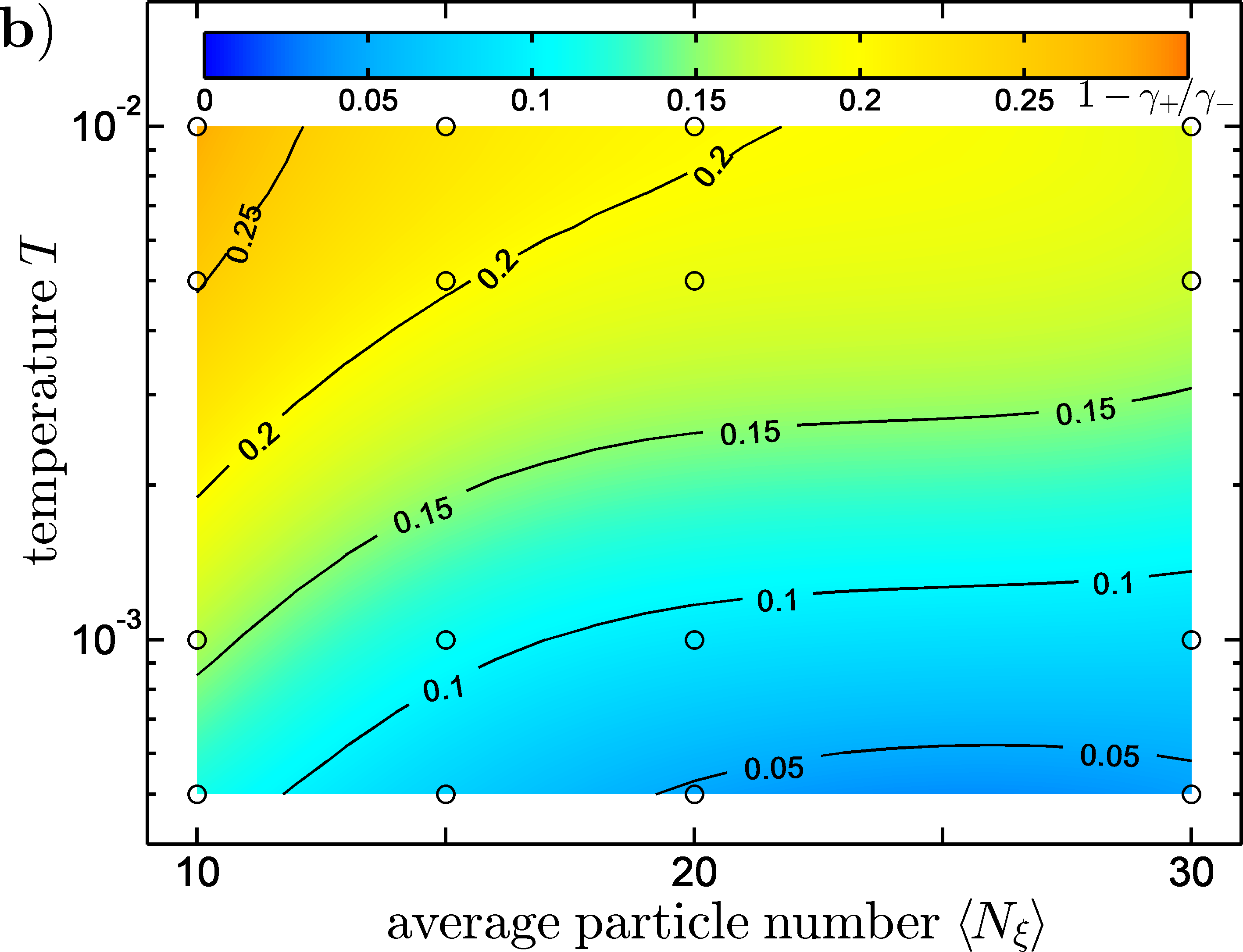
Figure 6 shows the interfacial tension derived with the Kirkwood–Buff formula eqn. (26) over a range of control parameters $\left\langle N_{\xi}\right\rangle$ and $T$. While panel (a) shows the interfacial tension for a $\rm{SRD}^{mc}_{+}$ fluid, panel (b) shows the relative difference of the interfacial tension between $\rm{SRD}^{mc}_{+}$ and $\rm{SRD}^{mc}_{-}$ fluids, respectively. For the considered control parameters the interfacial tension for $\rm{SRD}^{mc}$ fluids increases with increasing $\left\langle N_{\xi}\right\rangle$ and $T$ where the dependence on $T$ is stronger than on $\left\langle N_{\xi}\right\rangle$. The values for $\rm{SRD}^{mc}_{-}$ fluids differ by $\approx 25\%$ compared to those of $\rm{SRD}^{mc}_{+}$ fluids if $T$ is high and $\left\langle N_{\xi}\right\rangle$ is low. The lower the temperature and the higher the average particle number, the smaller is the difference between the interfacial tension of $\rm{SRD}^{mc}_{+}$ and $\rm{SRD}^{mc}_{-}$ fluids ($<5\%$).

The increase of interfacial tension with increasing temperature correlates well with the strength of the depletion layer created at an interface (see Fig. 4). If the temperature is low and correspondingly the mean free path of the particles is short a smaller interfacial tension is needed to counterbalance the flux of particles towards the interface. Similarly, if the temperature is high a stronger interfacial tension is needed to counterbalance the particle flux. This also means that it is not possible to arbitrarily tune the interfacial tension in a $\rm{SRD}^{mc}$ system. If the mean free path is too short (low temperatures in our case) it may happen that collision cells contain no particles and therefore any hydrodynamical behavior is lost. On the contrary, if the mean free path is too long (high temperatures in our case) the phase segregation is no longer stable. Particles of one phase may end up after the velocity update and next streaming step inside the other phase and effectively rupture the interface. If we assume that the interface is stable up to a mean free path of $\lambda_{\rm MFP}\approx 0.5a$ then the upper limit for the system temperature in our setup would be $T\approx 0.25$. The effect of the depletion layer is addressed again in Sec. 4.4 when we study the slip between two fluid phases. We like to point out that the phase segregation of the $\rm{SRD}^{mc}$ operator is most effective if thermal fluctuations are low and the system is in the collisional–dominated regime and therefore the collisional part in the stress tensor dominates over the advective part.

An alternative to the interfacial tension measurements from a microscopic stress profile employs the Young–Laplace equation $\Delta P=2\gamma/R$, where $R$ is the radius of a spherical droplet of fluid A in mechanical equilibrium with the ambient fluid B. Measurements of the difference $\Delta P\equiv P_{A}-P_{B}$ of bulk pressures $P_{i}$ in the fluids $i=A,B$ allows us to infer the interfacial tension $\gamma$ from the constant of proportionality between $\Delta P$ and the curvature $R^{-1}$ of the interface. This method has been used before to determine $\gamma$ in two–phase SRD fluids [1, 51]

We perform the Young–Laplace test as a further benchmark of the values obtained by the planar interface method outlined in Fig. 6. Due to high symmetry of the droplet, we employ a cubic simulation box of size $L^{3}=64^{3}$ with periodic boundary conditions, and apply the standard control parameter temperature $T=5\times 10^{-3}$ and average particle number $\left\langle N_{\xi}\right\rangle=15$. Different sized spherical droplets of fluid A are placed in the center of the box while the remaining space is uniformly filled with particles of fluid B. In line with the simulations described before (Sec. 4.1), we obtain time averages of all measured quantities for a duration of $5\times 10^{4}$ time steps. Before this measurement interval we waited for $2\times 10^{4}$ time steps to ensure a sufficient equilibration of the droplet and the ambient fluid. During the measurement interval the pressure $P_{A}$ and $P_{B}$ in the bulk fluids is determined by the area–weighted averaging method as described in Sec. 2.4. The results are shown in Fig. 7a.

Due to the Brownian motion of the droplet, we displace all fluid particles in the simulation box in regular intervals by a shift $\mathbf{d}_{c}=\mathbf{x}_{\mathrm{CM}}-\mathbf{x}_{\mathrm{CS}}$ where $\mathbf{x}_{\mathrm{CM}}$ is the center of mass position of all fluid particles in the droplet, and $\mathbf{x}_{\mathrm{CS}}$ the center of the simulation box. This procedure avoids ‘smearing out’ of the relevant physical quantities by a diffusion of the droplet’s center of mass. The inset in Fig. 7a shows the particle density as a function of the radial distance from the center of mass $\left|\mathbf{x}-\mathbf{x}_{\mathrm{CM}}\right|$. The dashed lines are the individual color densities and the solid black line is the total particle density, respectively. The radius of the equilibrated droplet is taken to be the crossing point of the individual color densities (vertical gray dashed line). The width of the interface is approximately one lattice unit which is the intrinsic length scale determined by the collision operator. The inset of Fig. 7a also illustrates the density difference between the droplet and the ambient bulk phase created by the self–compression of the droplet phase.

In the example above the initial radius of the droplet is $R_{\mathrm{i}}=12a$. Because of self–compression the particle density inside the droplet is approx. $7\%$ higher and the final radius of the equilibrated droplet is $R_{f}=11.89a<R_{i}$. Due to the fact that a $\rm{SRD}^{mc}$ fluid is rather a gas than a liquid the smaller the droplet radius and therewith the larger the curvature of the droplet, the larger is the density difference between the droplet and the bulk. The density difference between the two phases is directly linked to the pressure difference by the ideal gas law. We will account for the density difference in the course of this section when we determine the interfacial tension from the Young–Laplace equation. In Fig. 7a the pressure difference $\Delta P$ between droplet and bulk is shown as a function of the inverse equilibrated radius $R^{-1}$. The solid black line displays the result of a linear fit to the simulation data. The interfacial tension derived from this fit deviates by almost $10\%$ from the interfacial tension measured with the planar interface method (red dashed line).

To account for the dependence of the interfacial tension $\gamma$ on the particle densities $n_{A}$ and $n_{B}$ in the adjacent bulk fluids, we expand $\gamma(n_{A},n_{B})$ in a Taylor series in powers of the density difference $\Delta n=n_{A}-n_{B}$:

where $\bar{n}=(n_{A}+n_{B})/2$ is the average particle number. We can readily identify $\gamma_{0}(\bar{n})$ as the interfacial tension of a plane interface between two bulk phases of equal density $\bar{n}$ and an empirical constant $C(\bar{n})$. Both functions $\gamma_{0}(\bar{n})$ and $C(\bar{n})$ have to be determined from the simulation data. Odd terms in the Taylor expansion in eqn. (28) must vanish because the symmetry $\kappa_{AB}=\kappa_{BA}$ of weights in the $\rm{SRD}^{mc}$ collision operator implies $\gamma(n_{A},n_{B})=\gamma(n_{B},n_{A})$.

Using the relation $n_{i}=P_{i}/k_{B}T$ for an ideal gas, we can rewrite the Young–Laplace equation as an implicit equation

in the density difference $\Delta n$ which can be solved with expansion eqn. (28) in form of a power series in the curvature $R^{-1}$. After reexpressing the density difference by the pressure difference, we finally arrive at the relation

In the present study, we neglect all higher order terms $\sim{\cal O}(R^{5})$ and fit the cubic expression eqn. (30) in the curvature $R^{-1}$ to the simulation data, cf. the dashed black line in Fig. 7a. The zeroth order value $\gamma_{0}$ deviates by less than $0.4\%$ from the interfacial tension $\gamma_{planar}$ measured from the microscopic stress profile of the planar interface. As expected, for large droplets and hence small curvatures, the interfacial tension values approach the value for the planar interface in the asymptotic limit of zero curvature. Only the relation in eqn. (30) accounts for the increased density difference when considering small droplets which is reflected in the quality of the fit.

We determined the zeroth order interfacial tension $\gamma_{0}$ from fits according to eqn. (30) for the range of control parameters $T$ and $\left\langle N_{\xi}\right\rangle$ used in the computation of $\gamma_{planar}$ shown in Fig. 6a. The maximum relative difference between $\gamma_{planar}$ and $\gamma_{0}$ with $(0.8\pm 0.4)\%$ turns out the be very small.

Interfacial tension counteracts an increase of surface area and, thus, suppresses the roughening of a fluid–fluid interface by thermal fluctuations [83, 84, 85]. Fourier amplitudes $h_{\mathbf{k}}$ of the displacement field $h(\mathbf{r})$ measured with respect to an initially flat configuration contribute according to the equipartition theorem

leading to an RMS roughness proportional to $\sqrt{k_{B}T/\gamma}$. Figure 7b displays averages $\langle|h_{\mathbf{k}}|^{2}\rangle$ of an expansion into planar capillary waves as a function of the wave number $k$. The system parameters for this example are again $T=5\times 10^{-3}$ and average particle number is $\left\langle N_{\xi}\right\rangle=15$. Apart from the cut off at large wave vectors $k_{max}\approx\pi/a$, the data points for the three different simulation box sizes $L^{3}\in\{64^{3},128^{3},256^{3}\}$ conform to the characteristic power–law scaling in eqn. (31) in $k$ with an exponent $-2$. The dashed line shows the expected relation eqn. (31) with the value $\gamma_{planar}$ from the interfacial tension measurement. Deviations from the ideal scaling for small wave numbers can be attributed to the poor statistics for large wave lengths.

We used three independent methods to determine the interfacial tension between two $\rm{SRD}^{mc}$ fluids. We could show that the model correctly reproduces thermal fluctuations of the interface and that the interfacial tension can readily be determined with one of the above methods for any given set in the range of control parameters tested.

As we have shown before for the planar symmetry (Sec. 4.1) and the Young–Laplace test (Sec. 4.2), a depletion layer of lower particle density develops between two $\rm{SRD}^{mc}$ phases. This is due to the very nature of the multi–color algorithm and cannot be avoided. To elucidate how this depletion layer effects the interface behavior we perform again a shear experiment as described in Sec. 3. In contrast to the mono–phase experiments this time the system is half–filled with phase A ($z_{A}\in[-L_{z}/2,0]$) and half–filled with phase B ($z_{B}\in{]0,L_{z}/2]}$). Lees–Edwards boundary conditions are again applied in $z$–direction. The parameter range is the same as used before and angular momentum conservation is switched on ($\rm{SRD}^{mc}_{+}$).

Figure 8a shows velocity profiles of two examples out of the set with two different temperatures ($\mathrm{T_{1}}=5\times 10^{-4}$ and $\mathrm{T_{2}}=5\times 10^{-3}$). For the sake of clarity, only the $y$– and $z$–components of the velocity are indicated for $\mathrm{T_{1}}$. The inset in Fig. 8a magnifies the $x$–component of the velocity profiles around $z=0$. Clearly visible is the offset for $\mathrm{T_{1}}$ (black curve) corresponding to an interfacial slip between the two fluid phases. An extrapolation length similar to the Navier slip length can be defined by first extrapolating the velocity profiles in both bulk fluids to the lateral position $x_{0}^{A}$ and $x_{0}^{B}$ with $v_{z}(x_{0}^{A,B})=0$, and then defining the slip length $b$ as the difference $b=x_{0}^{A}-x_{0}^{B}a$. For a small temperature $\mathrm{T_{1}}$, the interfacial slip length is $b=(0.89\pm 0.02)a$ which is in the order of the spatial range of the $\rm{SRD}^{mc}$ operator. When increasing the temperature by an order of magnitude to $\mathrm{T_{2}}$ (red curve) the interfacial slip length reduces significantly to $b=(0.17\pm 0.01)a$. This weak slip is almost no longer visible in Fig. 8a as well as in the inset. Figure 8b shows the interfacial slip as a function of average particle number $\left\langle N_{\xi}\right\rangle$ and temperature $T$ for the complete parameter range. As expected from the planar symmetry test (Sec. 4.1) the interfacial slip depends much stronger on temperature than on average particle number. At high temperatures the amplitude of the depletion layer is rather small and momentum can effectively be transported across the interface leading to a reduced slip length $b$. Therefore, the same arguments hold for the interfacial slip as well as for the slip on solid walls. An increase in temperature leads to a decrease of the slip length and vice versa [68].

A good trade–off between the unphysical slip at the interface and a possible rupturing is reached at temperatures of $T\approx 5\times 10^{-3}$. Hence, we will use this temperature value throughout the following simulations.

Multi–phase flows are characterized by an interplay of inertial, viscous, and capillary forces. The relative magnitude of these forces is described by two non–dimensional numbers, the capillary number $Ca\equiv\eta U/\gamma$ and the Reynolds number $Re\equiv\rho UL^{\ast}/\eta$ where $U$ and $L^{\ast}$ are the characteristic velocity and length scale of the flow, respectively. In the regime of small $Ca\ll 1$, capillary forces dominate over viscous forces while small Reynolds numbers $Re\ll 1$ indicate that inertia can be neglected as compared to viscous forces. In the limit $Re\ll 1$, we can assume that capillary and viscous stresses are in equilibrium at any point in time.

To test whether the $\rm{SRD}^{mc}_{+}$ algorithm correctly reproduces the interplay between capillary, viscous and inertial forces, we studied the steady deformation of a viscous drop subjected to a linear shear flow. The deformation of drops in different flow fields was first studied in the pioneering experiments of Taylor [86, 87]. Depending on the viscosity ratio, the drop not only deforms under the influence of the incident shear flow but also disintegrates above a certain shear rate into smaller daughter droplets. The dynamics of drop breakup in shear flow was studied experimentally and numerically by e.g. [88, 89, 90]. It is beyond the scope of this work to examine the whole variety of deformation and breakup patterns in view of the particular predictions of the models but we refer the reader to the overview work of Ref. [91].

Deformations of a single droplet in a linear shear flow depend on the radius $R$ of the undeformed, spherical drop and its dynamic viscosity $\eta_{d}$ and mass density $\rho_{d}=m_{d}\,n$, the density $\rho_{b}=m_{b}\,n$ and the dynamic viscosity $\eta_{b}$ of the ambient fluid phase, the interfacial tension $\gamma$, and the asymptotically reached shear rate $\dot{\gamma}=\partial_{z}v_{x}$ far away from the droplet. Hence, the relevant dimensionless control parameters are the ratio of drop and bulk viscosities $\lambda^{\ast}\equiv\eta_{d}/\eta_{b}$, the capillary number $Ca\equiv\dot{\gamma}\eta_{b}R/\gamma$ and the Reynolds number $Re=\dot{\gamma}\rho_{b}R^{2}/\eta_{b}$. The Taylor deformation parameter of the drop is determined by $D\equiv(L_{d}-l_{d})/(L_{d}+l_{d})$ where $L_{d}$ and $l_{d}$ are the long and short axis of the deformed drop respectively. An undeformed, spherical droplet corresponds to a deformation parameter $D=0$ while $D\rightarrow 1$ if the droplet is unboundedly stretched.

In its simplest form the different stages of deformation of a viscous drop in simple linear shear flow can be characterized by the Reynolds number $Re$ and capillary number $Ca$, respectively. For low Reynolds numbers $Re\rightarrow 0$, i.e. in the Stokes flow limit, and for a viscosity ratio of $\lambda^{\ast}=1$, a critical capillary number $Ca^{*}\approx 0.42$ is found. For this particular viscosity ratio, the deformation of the droplet is approximately ellipsoidal until it reaches the limit $Ca^{*}$ where it breaks up into smaller droplets. For large viscosity ratios $\lambda^{\ast}\gtrsim 4$, the droplet reaches an maximum elongation $D^{max}$ and does not disintegrate as $Ca$ is further increased unless the Reynolds number $Re$ becomes comparable to unity [90].

Increase of the shear rate $\dot{\gamma}$ leads to an increase of the Reynolds number $Re\propto Ca$ where the ratio between $Re$ and $Ca$ is given by the Ohnesorge number $Oh^{-2}=Re/Ca$ which relates viscous to inertial forces. The critical capillary number $Ca^{*}$ of break up itself depends on $Re$ since the acceleration of the fluid particles in the rotating droplet and continuous fluid counteracts the stabilizing capillary stresses. Consequently, the critical capillary number is lowered $Ca^{*}(Re)<Ca^{*}(Re=0)$ limiting the range of stable, stationary droplet shapes as it has been numerically explored in Ref [92].

We simulated two benchmark scenarios where in one the viscosity ratio between the drop and the bulk fluid is $\lambda^{\ast}\approx 1$ and in the other $\lambda^{\ast}\approx 4$ with the following system parameters. For both benchmarks the initial radius of the drop is $R=8a$ and the drop is placed as a sphere in the center of the domain. The system size is $L=16R\times 8R\times 8R$ which is large enough to avoid any boundary effects [93]. We apply again periodic boundary conditions in $x$– and $y$–direction and Lees–Edwards boundary conditions in $z$–direction (see Sec. 3). The system temperature $T=5\times 10^{-3}$ and average particle number $\left\langle N_{\xi}\right\rangle=15$ is kept constant in all simulations. For $\lambda^{\ast}\approx 1$ all particles have mass $m=1$ whereas for $\lambda^{\ast}\approx 4$ the mass of the drop particles is increased to $m=5$ leading to an increase of viscosity by a factor of $\approx 4$ (see also Sec. 3). All systems are equilibrated for $2\times 10^{4}$ time steps until the velocity field is stable and afterwards the drop shape is averaged over $5\times 10^{4}$ subsequent time steps.

Shapes of the tank–treading drops in steady–state are summarized in Fig. 9. For small shear rates in panels (a) and (b) of Fig. 9, the shapes are almost perfectly ellipsoidal. Drops at larger shear rates with stronger deformations in panels (c) and (d) of Fig. 9 tend to be more elongated. Deformation $D$ is plotted against the capillary number $Ca$ in Fig. 9e for $\lambda^{\ast}\approx 1$ (blue symbols) and $\lambda^{\ast}\approx 4$ (red symbols). Additionally, the dashed line shows the linear relation for small droplet deformations from Refs. [86, 87] given by

for $\lambda^{\ast}=1$ and $Re=0$. The black symbols in Fig. 9e are taken from Ref. [92] where the authors compare different numerical implementations of this problem for $\lambda^{\ast}=1$ and $Re=0$. For small capillary numbers up to $Ca\approx 0.1$ the $\rm{SRD}^{mc}_{+}$ simulations show the same linear relation as presented by other authors [87, 92]. If the capillary number is increased the $\rm{SRD}^{mc}_{+}$ simulations with $\lambda^{\ast}\approx 1$ and $\lambda^{\ast}\approx 4$ show a strong deformation already at relatively small capillary numbers. Furthermore, also the drop breakup occurs at smaller capillary numbers of $Ca\approx 0.24$. In the inset in Fig. 9e we show the Reynolds number $Re$ and capillary number $Ca$ for our two benchmark sets. The dashed line in the inset is taken from Ref. [92] and marks a stability regime for the case $\lambda^{\ast}=1$ (blue symbols in our case) where drops are stable for small $Ca$ and small $Re$ (region left of the line). For small $Ca$ much larger values for $Re$ are needed before the drop breaks up into daughter droplets. Because in our $\rm{SRD}^{mc}_{+}$ simulations $Re\propto Ca$, the systems are not in the Stokes flow limit of $Re=0$. In the inset in Fig. 9e one can see that all but the last two of the data points for the case $\lambda^{\ast}\approx 1$ (blue circles) are below the breakup line. Considering the larger error bars especially for that last point (larger fluctuations) it may be that this drop also breaks up for longer simulation times. Blue crosses indicate drops that are unstable and have disintegrated into smaller droplets. A larger viscosity ratio (red symbols) counteracts increasing $Re$ and stable droplet shapes with stronger deformations are possible which is also indicated by a decreasing Ohnesorge number. This corresponds to the findings of e.g. Ref. [87] that for $Re\ll 1$ and $\lambda^{\ast}\gtrsim 4$ drop breakup no longer occurs no matter how large $Ca$ is.

This short example shows the capability of the $\rm{SRD}^{mc}_{+}$ algorithm to be used to study deforming droplets in linear shear flow at finite $Re$ numbers. Especially, the possibility to alter the viscosity ratio between the drop and the bulk fluid may be of interest for future studies.

Different affinities of the immiscible fluid phases to solid walls are controlled in our multi–color model through a virtual fluid phase inside the walls. These virtual fluid particles have been introduced already in Sec. 2.1 to enforce the no–slip boundary condition for a mono–phase fluid in cases where the mean free path is small compared to the size of the collision cells. The adhesion strength of a droplet in contact to the wall can be controlled if we assign the virtual particles a certain color. Still, the virtual wall particles do not participate in the streaming step. Instead, they are removed and created anew after or before every collision step, respectively. Full wetting conditions are reached if we assign all virtual particles the color of the droplet phase. Likewise, the droplet is fully non–wetting if all virtual particles are assigned the color of the ambient fluid phase. Partial wetting of the fluid phases is achieved in a certain range of mixing ratios of virtual particles with colors of either the droplet or the continuous phase. Once a mechanical equilibrium is reached, the fluid–fluid interface of the droplet intersects the solid wall at a certain contact angle $\theta$. Besides a dependence on the control parameter $T$ and $\left\langle N_{\xi}\right\rangle$, the equilibrium contact angle will be a function of the color ratio

where $N_{A}$ is the amount of virtual particles with the color of the bulk fluid and $N_{B}$ the amount of virtual particles with the color of the droplet, respectively. The corresponding contact angles $\theta$ need to be determined from a series of simulations.

To determine the dependence of the contact angle $\theta$ on the ratio $\lambda_{\mathrm{VP}}$ we perform the following experiment. In a cubic simulation box of size $L^{3}=32^{3}$ with periodic boundary conditions in $x$– and $y$–direction and bounce–back boundary conditions in $z$–direction a spherical cap–shaped droplet is placed at the center of the lower $z$–surface at $L_{z}=0$ with a radius of $R=7a$. The temperature of the system is $T=5\times 10^{-3}$ and the average particle number is $\left\langle N_{\xi}\right\rangle=20$. Because the average particle number in the simulation box is the same as inside the walls it is possible to measure 21 configurations of a partially wetting droplet in mechanical equilibrium. The contact angle $\theta$ is measured in the following manner. The time averaged droplet interface is fitted with a spherical cap to determine the radius $R$ and the height $h$ (see inset in Fig. 10b). From these fitted values $\theta$ is calculated with

Figure 10a exemplifies the evolution of the contact angle $\theta$ over time for five different ratios of $\lambda_{\mathrm{VP}}$. The equilibrium contact angle is already reached after a maximum of $2\>000$ time steps. After this initial time span the contact angle is stable within small fluctuations for the remainder of the simulation. Figure 10b shows the cosine of the final contact angle as a function of $\lambda_{\mathrm{VP}}$. The plotted value is a time average over $2\times 10^{4}$ time steps taken after $2\times 10^{4}$ time steps of equilibration of the data shown in Fig. 10a (dashed lines to the individual curves). The error bars show the standard deviation of the contact angle values over the averaging period. Other than for the two extreme cases where $\lambda_{\mathrm{VP}}=0$ and $\lambda_{\mathrm{VP}}=1$ the relationship between the contact angle and $\lambda_{\mathrm{VP}}$ is broadly linear. The small insets in Fig. 10b show the time averaged droplet interface (red) and the corresponding fit of the spherical cap (grid) for five different realizations. Note the remarkably well overlap of the interface and the fitted spherical cap. For the extreme cases $\lambda_{\mathrm{VP}}=0$ and $\lambda_{\mathrm{VP}}=1$, as expected, the droplet either completely wets the surface ($\cos{\theta_{0}}=1$) or detaches from the surface ($\cos{\theta_{1}}=-1$).

As a further benchmark to test whether the interfacial flows in contact to solid walls are faithfully reproduced in our $\rm{SRD}^{mc}$ implementation, we study the dewetting of a liquid droplet from a wettability pattern [94, 95, 96, 97]. A linear stripe of high wettability is created using spatial modulation of the color ratio of virtual wall particles in a rectangular region of a plane solid wall. A series of color ratios of virtual particles is chosen to achieve a low contact angle $\theta_{0}<90^{\circ}$ on the stripe, while the high contact angle on the surrounding surface is fixed to $\theta_{m}=180^{\circ}$. In the present study we consider a ratio $L_{\parallel}/L_{\perp}=42$ of stripe length $L_{\parallel}=256a$ to stripe width $L_{\perp}=8a$. A large simulation box with dimensions $256\times 32\times 32$ and periodic boundary conditions in $x$– and $y$–direction ensures that the shape evolution of the dewetting droplets are not affected by the finite size of the system. Initially, a flat cylindrical droplet of varying volume in the range of $V=1L^{3}_{\perp}$ to $V=10L^{3}_{\perp}$ is deposited on the stripe. Here, we chose the length of the droplet to be shorter than the stripe to avoid a connection of the wetting fluid phase across the periodic boundary. As a result, a fraction at the end of the stripe remains in contact to the ambient non–wetting fluid.

References

- [1] Y. Inoue, Y. Chen, H. Ohashi, A mesoscopic simulation model for immiscible multiphase fluids, J. Comput. Phys. 201 (2004) 191–203. doi:10.1016/j.jcp.2004.05.008.
- [2] Y. Inoue, S. Takagi, Y. Matsumoto, A mesoscopic simulation study of distributions of droplets in a bifurcating channel, Comput. Fluids 35 (2006) 971–977. doi:10.1016/j.compfluid.2005.07.018.
- [3] S. F. Kistler, P. M. Schweizer (Eds.), Liquid Film Coating: Scientific principles and their technological implications, Chapmann & Hall, 1997.
- [4] D. Bonn, J. Eggers, J. Indekeu, J. Meunier, E. Rolley, Wetting and spreading, Rev. Mod. Phys. 81 (2) (2009) 739–8005. doi:10.1103/RevModPhys.81.739.
- [5] N. R. Morrow, Wettability and Its Effect on Oil Recovery, J. Petrol. Technol. 42 (12) (1990) 1476–1484. doi:10.2118/21621-PA.
- [6] M. Sahimi, Flow and Transport in Porous Media and Fractured Rock: From Classical Methods to Modern Approaches, John Wiley & Sons, New York, 2001.
- [7] H. A. Stone, A. D. Stroock, A. Ajdari, ENGINEERING FLOWS IN SMALL DEVICES: Microfluidics Toward a Lab–on–a–Chip, Annu. Rev. Fluid Mech. 36 (2004) 381–411. doi:10.1146/annurev.fluid.36.050802.122124.
- [8] R. Seemann, M. Brinkmann, T. Pfohl, S. Herminghaus, Droplet based microfluidics, Rep. Prog. Phys. 75 (2012) 016601. doi:10.1088/0034-4885/75/1/016601.
- [9] Y. Sui, H. Ding, P. D. M. Spelt, Numerical Simulation of Flows with Moving Contact Lines, Annu. Rev. Fluid Mech. 46 (2014) 97–119. doi:10.1146/annurev-fluid-010313-141338.
- [10] P. J. Hoogerbrugge, J. M. V. A. Koelman, Simulating microscopic hydrodynamics phenomena with dissipative particle dynamics, Europhys. Lett. 19 (3) (1992) 155. doi:10.1209/0295-5075/19/3/001.
- [11] P. Español, P. Warren, Statistical mechanics of dissipative particle dynamics, Europhys. Lett. 30 (4) (1995) 191. doi:10.1209/0295-5075/30/4/001.
- [12] X. Shan, H. Chen, Lattice Boltzmann model for simulating flows with multiple phases and components, Phys. Rev. E: Stat., Nonlinear, Soft Matter Phys. 47 (3) (1993) 1815. doi:10.1103/PhysRevE.47.1815.
- [13] S. Chen, G. D. Doolen, Lattice Boltzmann Method for Fuid Flows, Annu. Rev. Fluid Mech. 30 (1998) 329–364. doi:10.1146/annurev.fluid.30.1.329.
- [14] S. Succi, The Lattice Boltzmann Equation for Fluid Dynamics and Beyond, Numerical Mathematics and Scientifc Computation, Oxford University Press, 2001.
- [15] A. Malevanets, R. Kapral, Mesoscopic model for solvent dynamics, J. Chem. Phys. 110 (17) (1999) 8605–8613. doi:10.1063/1.478857.
- [16] A. Malevanets, R. Kapral, Solute molecular dynamics in a mesoscale solvent, J. Chem. Phys. 112 (16) (2000) 7260–7269. doi:10.1063/1.481289.
- [17] R. Kapral, Multiparticle collision dynamcis: simulation of complex systems on mesoscales, Adv. Chem. Phys. 140 (2008) 89–146. doi:10.1002/9780470371572.ch2.
- [18] G. Gompper, T. Ihle, D. Kroll, R. G. Winkler, Multi–Particle Collision Dynamics: A Particle–Based Mesoscale Simulation Approach to the Hydrodynamics of Complex Fluids, in: C. Holm, K. Kremer (Eds.), Advanced Computer Simulation Approaches for Soft Matter Sciences III, Vol. 221 of Advances in Polymer Sciences, Springer Berlin Heidelberg, 2009, pp. 1–87. doi:10.1007/978-3-540-87706-6_1.
- [19] J. M. Haile, Molecular Dynamics Simulation, Wiley, New York, 1992.
- [20] R. Mittal, G. Iaccarino, Immersed Boundary Methods, Annu. Rev. Fluid Mech. 37 (2005) 239–261. doi:10.1146/annurev.fluid.37.061903.175743.
- [21] B. Kaoui, T. Krüger, J. Harting, How does confinement affect the dynamics of viscous vesicles and red blood cells?, Soft Matter 8 (35) (2012) 9246–9252. doi:10.1039/C2SM26289D.
- [22] M. Hecht, J. Harting, T. Ihle, H. J. Herrmann, Simulation of claylike colloids, Phys. Rev. E: Stat., Nonlinear, Soft Matter Phys. 72 (1) (2005) 011408. doi:10.1103/PhysRevE.72.011408.
- [23] J. T. Padding, A. A. Louis, Hydrodynamic interactions and Brownian forces in colloidal suspensions: Coarse–graining over time and length scales, Phys. Rev. E: Stat., Nonlinear, Soft Matter Phys. 74 (3) (2006) 031402. doi:10.1103/PhysRevE.74.031402.
- [24] I. O. Götze, H. Noguchi, G. Gompper, Relevance of angular momentum conservation in mesoscale hydrodynamics simulations, Phys. Rev. E: Stat., Nonlinear, Soft Matter Phys. 76 (2007) 046705. doi:10.1103/PhysRevE.76.046705.
- [25] T. Franosch, M. Grimm, M. Belushkin, F. M. Mor, G. Foffi, Resonances arising from hydrodynamic memory in Brownian motion, Nature 478 (2011) 85–88. doi:10.1038/nature10498.
- [26] C.-C. Huang, R. G. Winkler, G. Sutmann, G. Gompper, Semidilute Polymer Solutions at Equilibrium and under Shear Flow, Macromolecules 43 (23) (2010) 10107–10116. doi:10.1021/ma101836x.
- [27] C.-C. Huang, G. Gompper, R. G. Winkler, Effect of hydrodynamic correlations on the dynamics of polymers in dilute solution, J. Chem. Phys. 138 (2013) 144902. doi:10.1063/1.4799877.
- [28] E. Allahyarov, G. Gompper, Mesoscopic solvent simulations: Multiparticle–collision dynamics of three–dimensional flows, Phys. Rev. E: Stat., Nonlinear, Soft Matter Phys. 66 (2002) 036702. doi:10.1103/PhysRevE.66.036702.
- [29] A. Lamura, G. Gompper, Numerical study of the flow around a cylinder using multi–particle collision dynamics, Eur. Phys. J. E 9 (2002) 477–485. doi:10.1140/epje/i2002-10107-0.
- [30] J. T. Padding, A. A. Louis, Hydrodynamic and Brownian Fluctuations in Sedimenting Suspensions, Phys. Rev. Lett. 93 (22) (2004) 220601. doi:10.1103/PhysRevLett.93.220601.
- [31] I. O. Götze, G. Gompper, Flow generation by rotating colloids in planar microchannels, Europhys. Lett. 92 (6) (2010) 64003. doi:10.1209/0295-5075/92/64003.
- [32] I. O. Götze, G. Gompper, Dynamic self–assembly and directed flow of rotating colloids in microchannels, Phys. Rev. E: Stat., Nonlinear, Soft Matter Phys. 84 (3) (2011) 031404. doi:10.1103/PhysRevE.84.031404.
- [33] M. Ripoll, R. G. Winkler, G. Gompper, Star Polymers in Shear Flow, Phys. Rev. Lett. 96 (18) (2006) 188302. doi:10.1103/PhysRevLett.96.188302.
- [34] L. Cannavacciuolo, R. G. Winkler, G. Gompper, Mesoscale simulations of polymer dynamics in microchannel flows, Europhys. Lett. 83 (3) (2008) 34007. doi:10.1209/0295-5075/83/34007.
- [35] S. Frank, R. G. Winkler, Polyelectrolyte electrophoresis: Field effects and hydrodynamic interactions, Europhys. Lett. 83 (2008) 38004. doi:10.1209/0295-5075/83/38004.
- [36] K.-W. Lee, M. G. Mazza, Stochastic rotation dynamics for nematic liquid crystals, J. Chem. Phys. 142 (16) (2015) 164110. doi:10.1063/1.4919310.
- [37] H. Noguchi, G. Gompper, Fluid Vesicles with Viscous Membranes in Shear Flow, Phys. Rev. Lett. 93 (25) (2004) 258102. doi:10.1103/PhysRevLett.93.258102.
- [38] H. Noguchi, G. Gompper, Shape transitions of fluid vesicles and red blood cells in capillary flows, Proc. Natl. Acad. Sci. U. S. A. 102 (40) (2005) 14159–14164. doi:10.1073/pnas.0504243102.
- [39] J. L. McWhirter, H. Noguchi, G. Gompper, Flow–induced clustering and alignment of vesicles and red blood cells in microcapillaries, Proc. Natl. Acad. Sci. U. S. A. 106 (15) (2008) 6039–6043. doi:10.1073/pnas.0811484106.
- [40] S.-Y. Reigh, R. G. Winkler, G. Gompper, Synchronization and bundling of anchored bacterial flagella, Soft Matter 8 (2012) 4363–4372. doi:10.1039/C2SM07378A.
- [41] J. Elgeti, U. B. Kaupp, G. Gompper, Hydrodynamics of Sperm Cells near Surfaces, Biophys. J. 99 (2010) 1018–1026. doi:10.1016/j.bpj.2010.05.015.
- [42] D. J. Earl, C. M. Pooley, J. F. Ryder, I. Bredberg, J. M. Yeomans, Modeling microscopic swimmers at low Reynolds number, J. Chem. Phys. 126 (6) (2007) 064703. doi:10.1063/1.2434160.
- [43] I. O. Götze, G. Gompper, Mesoscale simulations of hydrodynamic squirmer interactions, Phys. Rev. E: Stat., Nonlinear, Soft Matter Phys. 82 (4) (2010) 041921. doi:10.1103/PhysRevE.82.041921.
- [44] M. Theers, R. G. Winkler, Synchronization of rigid microrotors by time–dependent hydrodynamic interactions, Phys. Rev. E: Stat., Nonlinear, Soft Matter Phys. 88 (2) (2013) 023012. doi:10.1103/PhysRevE.88.023012.
- [45] M. Theers, R. G. Winkler, Effects of thermal fluctuations and fluid compressibility on hydrodynamic synchronization of microrotors at finite oscillatory Reynolds number: a multiparticle collision dynamics simulation study, Soft Matter 10 (2014) 5894–5904. doi:10.1039/C4SM00770K.
- [46] T. Ihle, D. Kroll, Stochastic rotation dynamics: A Galilean–invariant mesoscopic model for fluid flow, Phys. Rev. E: Stat., Nonlinear, Soft Matter Phys. 63 (2001) 020201(R). doi:10.1103/PhysRevE.63.020201.
- [47] T. Ihle, D. Kroll, Stochastic rotation dynamics. I. Formalism, Galilean invariance, and Green–Kubo relations, Phys. Rev. E: Stat., Nonlinear, Soft Matter Phys. 67 (2003) 066705. doi:10.1103/PhysRevE.67.066705.
- [48] T. Ihle, D. Kroll, Stochastic rotation dynamics. II. Transport coefficients, numerics, and long–time tails, Phys. Rev. E: Stat., Nonlinear, Soft Matter Phys. 67 (2003) 066706. doi:10.1103/PhysRevE.67.066706.
- [49] Y. Hashimoto, Y. Chen, H. Ohashi, Immiscible real–coded lattice gas, Comput. Phys. Commun. 129 (2000) 56–62. doi:10.1016/S0010-4655(00)00092-8.
- [50] T. Sakai, Y. Chen, H. Ohashi, Real–coded lattice gas model for ternary amphiphilic fluids, Phys. Rev. E: Stat., Nonlinear, Soft Matter Phys. 65 (3) (2002) 031503. doi:10.1103/PhysRevE.65.031503.
- [51] E. Tüzel, G. Pan, T. Ihle, D. Kroll, Mesoscopic model for the fluctuating hydrodynamics of binary and ternary mixtures, Europhys. Lett. 80 (4) (2007) 40010. doi:10.1209/0295-5075/80/40010.
- [52] Y. Inoue, S. Takagi, Y. Matsumoto, A simulation model for amphiphilic molecules in a mesoscale solvent, Comput. Math. Appl. 55 (7) (2008) 1469–1480. doi:10.1016/j.camwa.2007.08.017.
- [53] E. Tüzel, M. Strauss, T. Ihle, D. M. Kroll, Transport coefficients for stochastic rotation dynamics in three dimensions, Phys. Rev. B: Condens. Matter Mater. Phys. 68 (2003) 036701. doi:10.1103/PhysRevE.68.036701.
- [54] T. Ihle, E. Tüzel, D. Kroll, Resummed Green–Kubo relations for a fluctuating fluid–particle model, Phys. Rev. E: Stat., Nonlinear, Soft Matter Phys. 70 (2004) 035701(R). doi:10.1103/PhysRevE.70.035701.
- [55] M. Ripoll, K. Mussawisade, R. G. Winkler, G. G., Low–Reynolds–number hydrodynamics of complex fluids by multi–particle–collision dynamics, Europhys. Lett. 68 (1) (2004) 106. doi:10.1209/epl/i2003-10310-1.
- [56] T. Ihle, E. Tüzel, D. Kroll, Equilibrium calculation of transport coefficients for a fluid–particle model, Phys. Rev. E: Stat., Nonlinear, Soft Matter Phys. 72 (2005) 046707. doi:10.1103/PhysRevE.72.046707.
- [57] C. M. Pooley, J. M. Yeomans, Kinetic Theory Derivation of the Transport Coefficients of Stochastic Rotation Dynamics, J. Phys. Chem. B 109 (14) (2005) 6505–6513. doi:10.1021/jp046040x.
- [58] E. Tüzel, T. Ihle, D. Kroll, Dynamic correlations in stochastic rotation dynamics, Phys. Rev. E: Stat., Nonlinear, Soft Matter Phys. 74 (5) (2006) 056702. doi:10.1103/PhysRevE.74.056702.
- [59] H. Noguchi, G. Gompper, Transport coefficients of off–lattice mesoscale–hydrodynamics simulation techniques, Phys. Rev. E: Stat., Nonlinear, Soft Matter Phys. 78 (2008) 016706. doi:10.1103/PhysRevE.78.016706.
- [60] R. G. Winkler, C. Huang, Stress tensors of multiparticle collision dynamics fluids, J. Chem. Phys. 130 (2009) 074907. doi:10.1063/1.3077860.
- [61] C. Huang, A. Chatterji, G. Sutmann, G. Gompper, R. G. Winkler, Cell–level canonical sampling by velocity scaling for multiparticle collision dynamics simulations, J. Comput. Phys. 229 (2010) 168–177. doi:10.1016/j.jcp.2009.09.024.
- [62] M. K. Petersen, J. B. Lechman, S. J. Plimpton, G. S. Grest, P. J. in ’t Veld, P. R. Schunk, Mesoscale hydrodynamics via stochastic rotation dynamics: Comparison with Lennard–Jones fluid, J. Chem. Phys. 132 (17) (2010) 174106. doi:10.1063/1.3419070.
- [63] J. K. Whitmer, E. Luijten, Fluid–solid boundary conditions for multiparticle collision dynamics, J. Phys.: Condens. Matter 22 (2010) 104106. doi:10.1088/0953-8984/22/10/104106.
- [64] S. Hanot, M. Belushkin, G. Foffi, Partial slip at fluid–solid boundaries by multiparticle collision dynamics simulations, Soft Matter 9 (2013) 291–296. doi:10.1039/c2sm26316e.
- [65] M. Theers, R. G. Winkler, Bulk viscosity of multiparticle collision dynamics fluids, Phys. Rev. E: Stat., Nonlinear, Soft Matter Phys. 91 (3) (2015) 033309. doi:10.1103/PhysRevE.91.033309.
- [66] N. Kikuchi, C. M. Pooley, J. F. Ryder, J. M. Yeomans, Transport coefficients of a mesoscopic fluid dynamics model, J. Chem. Phys. 119 (12) (2003) 6388–6395. doi:10.1063/1.1603721.
- [67] A. Lamura, G. Gompper, T. Ihle, D. Kroll, Multi–particle collision dynamics: Flow around a circular and a square cylinder, Europhys. Lett. 56 (3) (2001) 319–325. doi:10.1209/epl/i2001-00522-9.
- [68] D. S. Bolintineanu, J. B. Lechman, S. J. Plimpton, G. S. Grest, No–slip boundary conditions and forced flow in multiparticle collision dynamics, Phys. Rev. E: Stat., Nonlinear, Soft Matter Phys. 86 (2012) 066703. doi:10.1103/PhysRevE.86.066703.
- [69] H. Noguchi, G. Gompper, Transport coefficients of dissipative particle dynamics with finite time step, Europhys. Lett. 79 (2007) 36002. doi:10.1209/0295-5075/79/36002.
- [70] D. J. Evans, G. P. Morris, Shear Thickening and Turbulence in Simple Fluids, Phys. Rev. Lett. 56 (20) (1986) 2172–2175. doi:10.1103/PhysRevLett.56.2172.
- [71] C.-C. Huang, A. Varghese, G. Gompper, R. G. Winkler, Thermostat for nonequilibrium multiparticle–collision–dynamics simulations, Phys. Rev. E: Stat., Nonlinear, Soft Matter Phys. 91 (1) (2015) 013310. doi:10.1103/PhysRevE.91.013310.
- [72]
R. J. E. Clausius,
On a
mechanical theorem applicable to heat, Philos. Mag. Ser. 4 40 (265) (1870)
122–127.
doi:10.1080/14786447008640370.
URL http://www.tandfonline.com/doi/pdf/10.1080/14786447008640370 - [73] C. R. A. Catlow, S. C. Parker, M. P. Allen, Computer Modeling of Fluids Polymers and Solids, Vol. 293 of NATO ASI Series, Kluwer Academic Publishers, 1990. doi:10.1007/978-94-009-2484-0.
- [74] B. D. Todd, D. J. Evans, P. J. Daivis, Pressure tensor for inhomogeneous fluids, Phys. Rev. E: Stat., Nonlinear, Soft Matter Phys. 52 (2) (1995) 1627–1638. doi:10.1103/PhysRevE.52.1627.
- [75] H. Heinz, W. Paul, K. Binder, Calculation of local pressure tensors in systems with many–body interactions, Phys. Rev. E: Stat., Nonlinear, Soft Matter Phys. 72 (2005) 066704. doi:10.1103/PhysRevE.72.066704.
- [76] J. H. Irving, J. G. Kirkwood, The Statistical Mechanical Theory of Transport Processes. IV. The Equations of Hydrodynamics, J. Chem. Phys. 18 (6) (1950) 817–829. doi:10.1063/1.1747782.
- [77] P. Schofield, J. Henderson, Statistical Mechanics of Inhomogeneous Fluids, Proc. Roy. Soc. Lond. A 379 (1776) (1982) 231–246. doi:10.1098/rspa.1982.0015.
- [78] A. Lees, S. Edwards, The computer study of transport processes under extreme conditions, J. Phys. C Solid State 5 (1972) 1921–1929. doi:10.1088/0022-3719/5/15/006.
- [79] J. G. Kirkwood, F. P. Buff, The Statistical Mechanical Theory of Surface Tension, J. Chem. Phys. 17 (3) (1949) 338–343. doi:10.1063/1.1747248.
- [80] J. S. Rowlinson, B. Widom, Molecular Theory of Capillarity, Clarendon, Oxford, 1982.
- [81] J. P. R. B. Walton, D. J. Tildesley, J. S. Rowlinson, J. R. Henderson, The pressure tensor at the planar surface of a liquid, Mol. Phys. 48 (6) (1983) 1357–1368. doi:10.1080/00268978300100971.
- [82] F. Varnik, J. Baschnagel, K. Binder, Molecular dynamics results on the pressure tensor of polymer films, J. Chem. Phys. 113 (10) (2000) 4444–4453. doi:10.1063/1.1288390.
- [83] S. A. Safran, Statistical Thermodynamics of Surfaces, Interfaces, and Membranes, Addison–Wesley, 1994.
- [84] E. G. Flekkoy, D. H. Rothman, Fluctuating Fluid Interfaces, Phys. Rev. Lett. 75 (2) (1995) 260–263. doi:10.1103/PhysRevLett.75.260.
- [85] E. G. Flekkoy, D. H. Rothman, Fluctuating hydrodynamic interfaces: Theory and simulation, Phys. Rev. E: Stat., Nonlinear, Soft Matter Phys. 53 (2) (1996) 1622. doi:10.1103/PhysRevE.53.1622.
- [86] G. I. Taylor, The Viscosity of a Fluid Containing Small Drops of Another Fluid, Proc. Roy. Soc. Lond. A 138 (1932) 41–48. doi:10.1098/rspa.1932.0169.
- [87] G. I. Taylor, The Formation of Emulsions in Definable Fields of Flow, Proc. Roy. Soc. Lond. A 146 (1934) 501. doi:10.1098/rspa.1934.0169.
- [88] B. J. Bentley, L. G. Leal, An experimental investigation of drop deformation and breakup in steady two–dimensional linear flows, J. Fluid Mech. 167 (1986) 241–283. doi:10.1017/S0022112086002811.
- [89] J. M. Rallison, A numerical study of the deformation and burst of a viscous drop in general shear flows, J. Fluid Mech. 109 (1981) 465–482. doi:10.1017/S002211208100116X.
- [90] J. M. Rallison, The deformation of small viscous drops and bubbles in shear flows, Annu. Rev. Fluid Mech. 16 (1984) 45–66. doi:10.1146/annurev.fl.16.010184.000401.
- [91] H. A. Stone, Dynamics of drop deformation and breakup in viscous fluids, Annu. Rev. Fluid Mech. 26 (1994) 65–102. doi:10.1146/annurev.fl.26.010194.000433.
- [92] J. Li, Y. Y. Renardy, M. Renardy, Numerical simulation of breakup of a viscous drop in simple shear flow through a volume–of–fluid method, Phys. Fluids 12 (2) (2000) 269–282. doi:10.1063/1.870305.
- [93] P. J. A. Janssen, P. D. Anderson, Boundary–integral method for drop deformation between parallel plates, Phys. Fluids 19 (4) (2007) 043602. doi:10.1063/1.2715621.
- [94] H. Gau, S. Herminghaus, P. Lenz, R. Lipowsky, Liquid Morphologies on Structured Surfaces: From Microchannels to Microchips, Science 283 (5398) (1999) 46–49. doi:10.1126/science.283.5398.46.
- [95] R. Lipowsky, P. S. Lenz, Peter Swain, Wetting and dewetting of structured and imprinted surfaces, Colloid. Surface A 161 (1) (2000) 3–22. doi:10.1016/S0927-7757(99)00321-0.
- [96] M. Brinkmann, R. Lipowsky, Wetting morphologies on substrates with striped surface domains, J. Appl. Phys. 92 (8) (2002) 4296–4306. doi:10.1063/1.1506003.
- [97] A. Klingner, F. Mugele, Electrowetting–induced morphological transitions of fluid microstructures, J. Appl. Phys. 95 (5) (2004) 2918. doi:10.1063/1.1643771.