跳到论文正文
W Papers独立论文阅读器 arXiv:1601.07674 论文正文 计算阅读时间 · 0%
引用这篇论文根据当前论文元数据生成,正式投稿前建议核对。


License: arXiv.org perpetual non-exclusive license
arXiv:1601.07674v1 [math.AP] 28 Jan 2016

Stability in the Energy Space of the Sum of NN Peakons for the Degasperis-Procesi Equation

André Kabakouala Affiliation: L.M.P.T., U.F.R Sciences et Techniques, Université de Tours, Parc Grandmont, Affiliation: 37200 Tours, France. Email: Andre.Kabakouala@lmpt.univ-tours.fr
Abstract

The Degasperis-Procesi equation possesses well-known peaked solitary waves that are called peakons. Their stability has been established by Lin and Liu in [5]. In this paper, we localize the proof (in some suitable sense detailed in Section 3) of the stability of a single peakon. Thanks to this, we extend the result of stability to the sum of NN peakons traveling to the right with respective speeds c1,…,cNc_{1},\ldots,c_{N}, such that the difference between consecutive locations of peakons is large enough.

1 Introduction

The Degasperis-Procesi (DP) equation

ut−ut​x​x+4​u​ux=3​ux​ux​x+u​ux​x​x,(t,x)∈ℝ+∗×ℝu_{t}-u_{txx}+4uu_{x}=3u_{x}u_{xx}+uu_{xxx},~~(t,x)\in\mathbb{R}^{*}_{+}\times\mathbb{R} (1.1)

is completely integrable (see [1]) and possesses, among others, the following invariants

E⁡(u)=∫ℝy​v​and​F​(u)=∫ℝu3,E(u)=\int_{\mathbb{R}}yv~~\text{and}~~F(u)=\int_{\mathbb{R}}u^{3}, (1.2)

where y=(1−∂x2)uy=(1-\partial^{2}_{x})u and v=(4−∂x2)−1uv=(4-\partial^{2}_{x})^{-1}u. Substituting uu by 4​v−vx​x4v-v_{xx} in (1.2) and using integration by parts (we suppose that u⁡(±∞)=v⁡(±∞)=vx​(±∞)=0u(\pm\infty)=v(\pm\infty)=v_{x}(\pm\infty)=0), the conservation laws can be rewritten as

E⁡(u)=∫ℝ(4​v2+5​vx2+vx​x2)​and​F​(u)=∫ℝ(−vx​x3+12​v​vx​x2−48​v2​vx​x+64​v3).E(u)=\int_{\mathbb{R}}\left(4v^{2}+5v^{2}_{x}+v^{2}_{xx}\right)~~\text{and}~~F(u)=\int_{\mathbb{R}}\left(-v^{3}_{xx}+12vv^{2}_{xx}-48v^{2}v_{xx}+64v^{3}\right). (1.3)

One can see that the conservation law E⁡(⋅)E(\cdot) is equivalent to ∥⋅∥2L2​(ℝ)\|\cdot\|^{2}_{L^{2}(\mathbb{R})}. Indeed, using integration by parts

‖u‖L2​(ℝ)2=∫ℝu2=∫ℝ(4​v−vx​x)2=∫ℝ(16​v2+8​vx2+vx​x2)≤4​E​(u),\|u\|^{2}_{L^{2}(\mathbb{R})}=\int_{\mathbb{R}}u^{2}=\int_{\mathbb{R}}(4v-v_{xx})^{2}=\int_{\mathbb{R}}\left(16v^{2}+8v^{2}_{x}+v^{2}_{xx}\right)\leq 4E(u), (1.4)

and applying Plancherel-Parseval identity

E⁡(u)=∫ℝy​v=∫ℝ1+ω24+ω2​|u^​(ω)|2≤∫ℝ|u^​(ω)|2=‖u‖L2​(ℝ)2,E(u)=\int_{\mathbb{R}}yv=\int_{\mathbb{R}}\frac{1+\omega^{2}}{4+\omega^{2}}|\widehat{u}(\omega)|^{2}\leq\int_{\mathbb{R}}|\widehat{u}(\omega)|^{2}=\|u\|^{2}_{L^{2}(\mathbb{R})}, (1.5)

where u^\widehat{u} denotes the Fourier transform of uu. In the sequel we will denote

‖u‖ℋ=E⁡(u).\|u\|_{\mathcal{H}}=\sqrt{E(u)}. (1.6)

Note that, by reversing the operator (1−∂x2)(⋅)(1-\partial^{2}_{x})(\cdot) in (1.1), the DP equation can be rewritten in conservation form as

ut+12∂xu2+32(1−∂x2)−1∂xu2=0,(t,x)∈ℝ+∗×ℝ.u_{t}+\frac{1}{2}\partial_{x}u^{2}+\frac{3}{2}(1-\partial^{2}_{x})^{-1}\partial_{x}u^{2}=0,~~(t,x)\in\mathbb{R}^{*}_{+}\times\mathbb{R}. (1.7)

The DP equation possesses solitary waves called peakons (see Fig. 1a) and defined by

u⁡(t,x)=φc​(x−c​t)=c​φ​(x−c​t)=c​e−|x−c​t|,c∈ℝ∗,(t,x)∈ℝ+∗×ℝ,u(t,x)=\varphi_{c}(x-ct)=c\varphi(x-ct)=ce^{-|x-ct|},~~c\in\mathbb{R}^{*},~~(t,x)\in\mathbb{R}^{*}_{+}\times\mathbb{R}, (1.8)

but they are not smooth since φc∉C1​(ℝ)\varphi_{c}\notin C^{1}(\mathbb{R}) (see Fig. 1b). The peakons are only global weak solutions of (1.7). It means, for any smooth test function ϕ∈C∞​(ℝ+×ℝ)\phi\in C^{\infty}(\mathbb{R}_{+}\times\mathbb{R}), it holds

∫0+∞∫ℝ\displaystyle\int_{0}^{+\infty}\int_{\mathbb{R}} φc​(x−c​t)​ϕt​(t,x)​𝑑t​𝑑x+12​∫0+∞∫ℝφc2​(x−c​t)​ϕx​(t,x)​𝑑t​𝑑x\displaystyle\varphi_{c}(x-ct)\phi_{t}(t,x)dtdx+\frac{1}{2}\int_{0}^{+\infty}\int_{\mathbb{R}}\varphi^{2}_{c}(x-ct)\phi_{x}(t,x)dtdx
+32∫0+∞∫ℝ(1−∂x2)−1φc2(x−ct)ϕx(t,x)dtdx+∫ℝφc(x)ϕ(0,x)dx=0.\displaystyle+\frac{3}{2}\int_{0}^{+\infty}\int_{\mathbb{R}}(1-\partial^{2}_{x})^{-1}\varphi^{2}_{c}(x-ct)\phi_{x}(t,x)dtdx+\int_{\mathbb{R}}\varphi_{c}(x)\phi(0,x)dx=0.

The goal of our work is to prove that ordered trains of peakons are stable under small perturbations in the energy space ℋ{\mathcal{H}} (equivalent to L2L^{2}).

Definition 1.1 (Stability).

Let c>0c>0 be given. The peakon φc\varphi_{c} is said stable in ℋ\mathcal{H}, if for all ε>0\varepsilon>0, there exists δ>0\delta>0 such that if

‖u0−φc‖ℋ≤δ,\|u_{0}-\varphi_{c}\|_{\mathcal{H}}\leq\delta, (1.9)

then for all t≥0t\geq 0, there exists ξ⁡(t)\xi(t) such that

∥u(t,⋅)−φc(⋅−ξ(t))∥ℋ≤ε,\|u(t,\cdot)-\varphi_{c}\left(\cdot-\xi(t)\right)\|_{\mathcal{H}}\leq\varepsilon, (1.10)

where u⁡(t)u(t) is the solution to (1.1) emanating from u0u_{0}.

Lin and Liu proved in [5] the stability of a single peakon under the additional condition that (1−∂x2)u0∈ℳ+(ℝ)(1-\partial^{2}_{x})u_{0}\in{\mathcal{M}}^{+}(\mathbb{R}). Using this result and the general strategy introduced by Martel, Merle and Tsai in [7] for the generalized Korteweg-de Vries (gKdV) equation and adapted by El Dika and Molinet in [3] and [2] for the Camassa-Holm (CH) equation, we prove here the stability of the sum of NN peakons for the DP equation.

Before stating the main result we introduce the function space where will live our class of solutions to the equation. For II a finite or infinite time interval of ℝ+\mathbb{R}_{+}, we denote by 𝒳⁡(I)\mathcal{X}(I) the function space 11 1 W1,1​(ℝ)W^{1,1}(\mathbb{R}) is the space of L1​(ℝ)L^{1}(\mathbb{R}) functions with derivatives in L1​(ℝ)L^{1}(\mathbb{R}) and B​V​(ℝ)BV(\mathbb{R}) is the space of function with bounded variation.

𝒳⁡(I)={u∈C⁡(I,H1​(ℝ))∩L∞​(I,W1,1​(ℝ)),ux∈L∞​(I,B​V​(ℝ))}.\mathcal{X}(I)=\left\{u\in C\left(I;H^{1}(\mathbb{R})\right)\cap L^{\infty}\left(I;W^{1,1}(\mathbb{R})\right),~u_{x}\in L^{\infty}\left(I;BV(\mathbb{R})\right)\right\}. (1.11)

The main result of the present paper is the following theorem.

Theorem 1.1 (Stability of the Sum of NN Peakons).

Let be given NN velocities c1,…,cNc_{1},\ldots,c_{N} such that 0<c1<…<cN0<c_{1}<\ldots<c_{N}. Let u∈𝒳([0,T[)u\in\mathcal{X}([0,T[), with 0<T≤+∞0<T\leq+\infty, be a solution of the DP equation. There exist C>0C>0, L0>0L_{0}>0 and ε0>0\varepsilon_{0}>0 only depending on the speeds (ci)i=1N(c_{i})_{i=1}^{N}, such that if

y0=(1−∂x2)u0∈ℳ+(ℝ)y_{0}=(1-\partial^{2}_{x})u_{0}\in\mathcal{M}^{+}(\mathbb{R}) (1.12)

and

‖u0−∑i=1Nφci(⋅−zi0)‖ℋ≤ε2,with0<ε<ε0,\left\|u_{0}-\sum_{i=1}^{N}\varphi_{c_{i}}(\cdot-z^{0}_{i})\right\|_{\mathcal{H}}\leq\varepsilon^{2},~~\text{with}~~0<\varepsilon<\varepsilon_{0}, (1.13)

for some z10,…,zN0z^{0}_{1},\ldots,z^{0}_{N} satisfying

z01<…<z0Nandz0i−z0i−1≥L,withL>L0>0,i=2,…,N,z^{0}_{1}<\ldots<z^{0}_{N}~~\text{and}~~z^{0}_{i}-z^{0}_{i-1}\geq L,~~\text{with}~~L>L_{0}>0,~~i=2,\ldots,N, (1.14)

then there exist ξ11​(t),…,ξ1N​(t)\xi^{1}_{1}(t),\ldots,\xi^{N}_{1}(t) such that

‖u(t)−∑i=1Nφci(⋅−ξ1i(t))‖ℋ≤C(ε+L−1/8),∀t∈[0,T[\left\|u(t)-\sum_{i=1}^{N}\varphi_{c_{i}}(\cdot-\xi^{i}_{1}(t))\right\|_{\mathcal{H}}\leq C(\sqrt{\varepsilon}+L^{-1/8}),~~\forall t\in[0,T[ (1.15)

and

ξ1i(t)−ξ1i−1(t)>L2,∀t∈[0,T[,i=2,…,N,\xi^{i}_{1}(t)-\xi^{i-1}_{1}(t)>\frac{L}{2},~~\forall t\in[0,T[,~~i=2,\ldots,N, (1.16)

where ξ11​(t),…,ξ1N​(t)\xi^{1}_{1}(t),\ldots,\xi^{N}_{1}(t) are defined in Subsection 4.1.

2 Preliminaries

In this section, we briefly recall the global well-posedness results for the DP equation and its consequences (see [4] and [6] for details).

Theorem 2.1 (Global Weak Solution; See [4] and [6]).

Assume that u0∈L2​(ℝ)u_{0}\in L^{2}(\mathbb{R}) with y0=(1−∂x2)u0∈ℳ+(ℝ)y_{0}=(1-\partial^{2}_{x})u_{0}\in\mathcal{M}^{+}(\mathbb{R}). Then the DP equation has a unique global weak solution u∈𝒳⁡(ℝ+)u\in\mathcal{X}(\mathbb{R}_{+}) such that

y(t,⋅)=(1−∂x2)u(t,⋅)∈ℳ+(ℝ),∀t∈ℝ+.y(t,\cdot)=(1-\partial^{2}_{x})u(t,\cdot)\in\mathcal{M}^{+}(\mathbb{R}),~~\forall t\in\mathbb{R}_{+}. (2.1)

Moreover E⁡(⋅)E(\cdot) and F⁡(⋅)F(\cdot) are conserved by the flow.

Remark 2.1 (Control of L∞L^{\infty} Norm by L2L^{2} Norm).

From (2.1), it holds

u⁡(x)=e−x2​∫−∞xex′​y​(x′)​d​x′+ex2​∫x+∞e−x′​y​(x′)​d​x′u(x)=\frac{e^{-x}}{2}\int_{-\infty}^{x}e^{x^{\prime}}y(x^{\prime})dx^{\prime}+\frac{e^{x}}{2}\int_{x}^{+\infty}e^{-x^{\prime}}y(x^{\prime})dx^{\prime}

and

ux(x)=−e−x2∫−∞xex′y(x′)dx′+ex2∫x+∞e−x′y(x′)dx′,u_{x}(x)=-\frac{e^{-x}}{2}\int_{-\infty}^{x}e^{x^{\prime}}y(x^{\prime})dx^{\prime}+\frac{e^{x}}{2}\int_{x}^{+\infty}e^{-x^{\prime}}y(x^{\prime})dx^{\prime},

which lead to

|ux​(x)|≤u⁡(x),∀x∈ℝ.|u_{x}(x)|\leq u(x),~~\forall x\in\mathbb{R}. (2.2)

Then, using the Sobolev embedding of H1​(ℝ)H^{1}(\mathbb{R}) into L∞​(ℝ)L^{\infty}(\mathbb{R}) and (2.2), we infer that there exists a constant CS>0C_{S}>0 such that

‖u‖L∞​(ℝ)≤CS​‖u‖H1​(ℝ)≤2​CS​‖u‖L2​(ℝ).\|u\|_{L^{\infty}(\mathbb{R})}\leq C_{S}\|u\|_{H^{1}(\mathbb{R})}\leq 2C_{S}\|u\|_{L^{2}(\mathbb{R})}. (2.3)
Lemma 2.1 (Positivity; See [6]).

Let u∈H1​(ℝ)u\in H^{1}(\mathbb{R}) with y=(1−∂x2)u∈ℳ+(ℝ)y=(1-\partial^{2}_{x})u\in\mathcal{M}^{+}(\mathbb{R}). If k1≥1k_{1}\geq 1, then we have

(k1±∂x)u(x)≥0,∀x∈ℝ.(k_{1}\pm\partial_{x})u(x)\geq 0,~~\forall x\in\mathbb{R}. (2.4)
Lemma 2.2 (Positivity; See [6]).

Let w(x)=(k1±∂x)u(x)w(x)=(k_{1}\pm\partial_{x})u(x). Assume that u∈H1​(ℝ)u\in H^{1}(\mathbb{R}) with y=(1−∂x2)u∈ℳ+(ℝ)y=(1-\partial^{2}_{x})u\in\mathcal{M}^{+}(\mathbb{R}). If k1≥1k_{1}\geq 1 and k2≥2k_{2}\geq 2, then we have

(k2±∂x)(4−∂x2)−1w(x)≥0,∀x∈ℝ.(k_{2}\pm\partial_{x})(4-\partial^{2}_{x})^{-1}w(x)\geq 0,~~\forall x\in\mathbb{R}. (2.5)

3 Stability of a single peakon

The proof of Lin and Liu in [5] is not entirely suitable for our work, because it involves all local extrema of the function v=(4−∂x2)−1uv=(4-\partial^{2}_{x})^{-1}u on ℝ\mathbb{R}, and thus is not local. For our work, we have to localize the estimates. Therefore, we need to modify a little the proof of Lin and Liu. We do this first for a single peakon.

Theorem 3.1 (Stability of Peakons).

Let u∈𝒳([0,T[)u\in\mathcal{X}([0,T[), with 0<T≤+∞0<T\leq+\infty, be a solution of the DP equation and φc\varphi_{c} be the peakon defined in (1.8), traveling to the right at the speed c>0c>0. There exist C>0C>0 and ε0>0\varepsilon_{0}>0 only depending on the speed c>0c>0, such that if

y0=(1−∂x2)u0∈ℳ+(ℝ)y_{0}=(1-\partial^{2}_{x})u_{0}\in\mathcal{M}^{+}(\mathbb{R}) (3.1)

and

‖u0−φc‖ℋ≤ε2,with​0<ε<ε0,\|u_{0}-\varphi_{c}\|_{\mathcal{H}}\leq\varepsilon^{2},~~\text{with}~~0<\varepsilon<\varepsilon_{0}, (3.2)

then

∥u(t,⋅)−φc(⋅−ξ1(t))∥ℋ≤Cε,∀t∈[0,T[,\|u(t,\cdot)-\varphi_{c}(\cdot-\xi_{1}(t))\|_{\mathcal{H}}\leq C\sqrt{\varepsilon},~~\forall t\in[0,T[, (3.3)

where ξ1​(t)∈ℝ\xi_{1}(t)\in\mathbb{R} is any point where the function v(t,⋅)=(4−∂x2)−1u(t,⋅)v(t,\cdot)=(4-\partial^{2}_{x})^{-1}u(t,\cdot) attains its maximum.

To prove this theorem we first need the following lemma that enables to control the distance of E⁡(u)E(u) and F⁡(u)F(u) to respectively E⁡(φc)E(\varphi_{c}) and F⁡(φc)F(\varphi_{c}).

Lemma 3.1 (Control of Distances Between Energies).

Let u∈H1​(ℝ)u\in H^{1}(\mathbb{R}) with y=(1−∂x2)u∈ℳ+(ℝ)y=(1-\partial^{2}_{x})u\in\mathcal{M}^{+}(\mathbb{R}). If ‖u−φc‖ℋ≤ε2\|u-\varphi_{c}\|_{\mathcal{H}}\leq\varepsilon^{2}, then

|E⁡(u)−E⁡(φc)|≤O⁡(ε2)|E(u)-E(\varphi_{c})|\leq O(\varepsilon^{2}) (3.4)

and

|F⁡(u)−F⁡(φc)|≤O⁡(ε2),|F(u)-F(\varphi_{c})|\leq O(\varepsilon^{2}), (3.5)

where O⁡(⋅)O(\cdot) only depends on the speed cc.

Proof. For the first estimate, applying triangular inequality, and using that ‖u−φc‖ℋ≤ε2\|u-\varphi_{c}\|_{\mathcal{H}}\leq\varepsilon^{2} and ‖φc‖ℋ=c/3\|\varphi_{c}\|_{\mathcal{H}}=c/\sqrt{3}, we have

|E⁡(u)−E⁡(φc)|\displaystyle|E(u)-E(\varphi_{c})| =|‖u∥ℋ−∥φc∥ℋ|(∥u∥ℋ+∥φc∥ℋ)\displaystyle=|\left\|u\|_{\mathcal{H}}-\|\varphi_{c}\|_{\mathcal{H}}\right|\left(\|u\|_{\mathcal{H}}+\|\varphi_{c}\|_{\mathcal{H}}\right)
≤‖u−φc‖ℋ​(‖u−φc‖ℋ+2​‖φc‖ℋ)\displaystyle\leq\|u-\varphi_{c}\|_{\mathcal{H}}\left(\|u-\varphi_{c}\|_{\mathcal{H}}+2\|\varphi_{c}\|_{\mathcal{H}}\right)
≤ε2​(ε2+2​c3)\displaystyle\leq\varepsilon^{2}\left(\varepsilon^{2}+\frac{2c}{\sqrt{3}}\right)
≤O⁡(ε2).\displaystyle\leq O(\varepsilon^{2}).

For the second estimate, applying the Hölder inequality, and using that ‖u−φc‖ℋ≤ε2\|u-\varphi_{c}\|_{\mathcal{H}}\leq\varepsilon^{2} and (2.3), we have

|F⁡(u)−F⁡(φc)|\displaystyle|F(u)-F(\varphi_{c})| ≤∫ℝ|u3−φc3|\displaystyle\leq\int_{\mathbb{R}}\left|u^{3}-\varphi^{3}_{c}\right|
≤∫ℝ|u−φc|​(u2+u​φc+φc2)\displaystyle\leq\int_{\mathbb{R}}|u-\varphi_{c}|(u^{2}+u\varphi_{c}+\varphi^{2}_{c})
≤‖u−φc‖L2​(ℝ)​(∫ℝ(u2+u​φc+φc2)2)1/2\displaystyle\leq\|u-\varphi_{c}\|_{L^{2}(\mathbb{R})}\left(\int_{\mathbb{R}}(u^{2}+u\varphi_{c}+\varphi^{2}_{c})^{2}\right)^{1/2}
=‖u−φc‖L2​(ℝ)​(∫ℝ(u4+2​u3​φc+3​u2​φc2+2​u​φc3+φc4))1/2\displaystyle=\|u-\varphi_{c}\|_{L^{2}(\mathbb{R})}\left(\int_{\mathbb{R}}(u^{4}+2u^{3}\varphi_{c}+3u^{2}\varphi^{2}_{c}+2u\varphi^{3}_{c}+\varphi^{4}_{c})\right)^{1/2}
≤‖u−φc‖L2​(ℝ)\displaystyle\leq\|u-\varphi_{c}\|_{L^{2}(\mathbb{R})}
⋅(4​CS2​‖u‖L2​(ℝ)4+4​c​CS​‖u‖L2​(ℝ)2+3​c2​‖u‖L2​(ℝ)2+83​c3​CS​‖u‖L2​(ℝ)+12​c4)1/2\displaystyle\hskip 28.45274pt\cdot\left(4C^{2}_{S}\|u\|^{4}_{L^{2}(\mathbb{R})}+4cC_{S}\|u\|^{2}_{L^{2}(\mathbb{R})}+3c^{2}\|u\|^{2}_{L^{2}(\mathbb{R})}+\frac{8}{3}c^{3}C_{S}\|u\|_{L^{2}(\mathbb{R})}+\frac{1}{2}c^{4}\right)^{1/2}
≤O⁡(ε2),\displaystyle\leq O(\varepsilon^{2}),

where we also use that the L2L^{2} norm of uu is bounded and the following measures of peakon:

‖φc‖L∞​(ℝ)=c,‖φc‖L3​(ℝ)=233​c​and​‖φc‖L4​(ℝ)=124​c.\|\varphi_{c}\|_{L^{\infty}(\mathbb{R})}=c,~~\|\varphi_{c}\|_{L^{3}(\mathbb{R})}=\sqrt[3]{\frac{2}{3}}c~~\text{and}~~\|\varphi_{c}\|_{L^{4}(\mathbb{R})}=\frac{1}{\sqrt[4]{2}}c.

This proves the lemma. □\square

Now, to prove Theorem 3.1, by the conservation of E⁡(⋅)E(\cdot), F⁡(⋅)F(\cdot) and the continuity of the map t↦u⁡(t)t\mapsto u(t) from [0,T[[0,T[ to H1​(ℝ)↪ℋH^{1}(\mathbb{R})\hookrightarrow\mathcal{H} (since ℋ≃L2\mathcal{H}\simeq L^{2} and ‖u‖L2​(ℝ)≤‖u‖H1​(ℝ)\|u\|_{L^{2}(\mathbb{R})}\leq\|u\|_{H^{1}(\mathbb{R})}), it suffices to prove that for any function u∈H1​(ℝ)u\in H^{1}(\mathbb{R}) satisfying y=(1−∂x2)u∈ℳ+(ℝ)y=(1-\partial^{2}_{x})u\in\mathcal{M}^{+}(\mathbb{R}), (3.4) and (3.5), if

infξ∈ℝ∥u−φc(⋅−ξ)∥ℋ≤ε1/4,\inf_{\xi\in\mathbb{R}}\|u-\varphi_{c}(\cdot-\xi)\|_{\mathcal{H}}\leq\varepsilon^{1/4}, (3.6)

then

∥u−φc(⋅−ξ1)∥ℋ≤Cε,\|u-\varphi_{c}(\cdot-\xi_{1})\|_{\mathcal{H}}\leq C\sqrt{\varepsilon}, (3.7)

where ξ1∈ℝ\xi_{1}\in\mathbb{R} is any point where the function v=(4−∂x2)−1uv=(4-\partial^{2}_{x})^{-1}u attains its maximum.

We divide the proof of Theorem 3.1 into a sequence of lemmas. In the sequel, we will need to introduce the following smooth-peakons defined for all x∈ℝx\in\mathbb{R} by:

ρc(x)=cρ(x)=(4−∂x2)−1φc(x)=c3e−|x|−c6e−2​|x|.\rho_{c}(x)=c\rho(x)=(4-\partial^{2}_{x})^{-1}\varphi_{c}(x)=\frac{c}{3}e^{-|x|}-\frac{c}{6}e^{-2|x|}. (3.8)

One can check that ρc∈H3​(ℝ)↪C2​(ℝ)\rho_{c}\in H^{3}(\mathbb{R})\hookrightarrow C^{2}(\mathbb{R}) (by the Sobolev embedding) since φc∈H1​(ℝ)\varphi_{c}\in H^{1}(\mathbb{R}). Indeed, we have

‖ρc‖H3​(ℝ)2=∫ℝ(1+ω2)3(4+ω2)2​|φ^c​(ω)|2≤∫ℝ(1+ω2)​|φ^c​(ω)|2≤‖φc‖H1​(ℝ)2=2​c2.\|\rho_{c}\|^{2}_{H^{3}(\mathbb{R})}=\int_{\mathbb{R}}\frac{(1+\omega^{2})^{3}}{(4+\omega^{2})^{2}}|\widehat{\varphi}_{c}(\omega)|^{2}\leq\int_{\mathbb{R}}(1+\omega^{2})|\widehat{\varphi}_{c}(\omega)|^{2}\leq\|\varphi_{c}\|^{2}_{H^{1}(\mathbb{R})}=2c^{2}. (3.9)

Moreover, ρc\rho_{c} is a positive even function which decays to 00 at infinity, and admits a single maximum c/6c/6 at point 00 (see Fig. 1a-1c).

Lemma 3.2 (Uniform Estimates).

Let u∈H1​(ℝ)u\in H^{1}(\mathbb{R}) with y=(1−∂x2)u∈ℳ+(ℝ)y=(1-\partial^{2}_{x})u\in\mathcal{M}^{+}(\mathbb{R}), and ξ∈ℝ\xi\in\mathbb{R}. If ∥u−φc(⋅−ξ)∥ℋ≤ε1/4\|u-\varphi_{c}(\cdot-\xi)\|_{\mathcal{H}}\leq\varepsilon^{1/4}, then

∥u−φc(⋅−ξ)∥L∞​(ℝ)≤O(ε1/8)\|u-\varphi_{c}(\cdot-\xi)\|_{L^{\infty}(\mathbb{R})}\leq O(\varepsilon^{1/8}) (3.10)

and

∥v−ρc(⋅−ξ)∥L∞​(ℝ)≤O(ε1/4),\|v-\rho_{c}(\cdot-\xi)\|_{L^{\infty}(\mathbb{R})}\leq O(\varepsilon^{1/4}), (3.11)

where v=(4−∂x2)−1uv=(4-\partial^{2}_{x})^{-1}u and ρc\rho_{c} is defined in (3.8).

Proof. For the second estimate, applying the Hölder inequality and using assumption, we get for all x∈ℝx\in\mathbb{R},

|v⁡(x)−ρc​(x−ξ)|\displaystyle\left|v(x)-\rho_{c}(x-\xi)\right| ≤14​∫ℝe−2​|x′|​|u⁡(x−x′)−φc​[(x−x′)−ξ]|​d​x′\displaystyle\leq\frac{1}{4}\int_{\mathbb{R}}e^{-2|x^{\prime}|}\left|u(x-x^{\prime})-\varphi_{c}\left[(x-x^{\prime})-\xi\right]\right|dx^{\prime}
≤14​(∫ℝe−4​|x′|​d​x′)1/2​(∫ℝ|u⁡(x′)−φc​(x′−ξ)|2​d​x′)1/2\displaystyle\leq\frac{1}{4}\left(\int_{\mathbb{R}}e^{-4|x^{\prime}|}dx^{\prime}\right)^{1/2}\left(\int_{\mathbb{R}}\left|u(x^{\prime})-\varphi_{c}(x^{\prime}-\xi)\right|^{2}dx^{\prime}\right)^{1/2}
≤12​2∥u−φc(⋅−ξ)∥ℋ\displaystyle\leq\frac{1}{2\sqrt{2}}\|u-\varphi_{c}(\cdot-\xi)\|_{\mathcal{H}}
≤O⁡(ε1/4).\displaystyle\leq O(\varepsilon^{1/4}).

For the first estimate, note that the assumption y=(1−∂x2)u≥0y=(1-\partial^{2}_{x})u\geq 0 implies that u=(1−∂x2)−1y≥0u=(1-\partial^{2}_{x})^{-1}y\geq 0 and satisfies (2.2). Then, applying triangular inequality, and using that |φc′|=φc|\varphi^{\prime}_{c}|=\varphi_{c} on ℝ\mathbb{R} and (2.3), we have

∥u−φc(⋅−ξ)∥H1​(ℝ)\displaystyle\|u-\varphi_{c}(\cdot-\xi)\|_{H^{1}(\mathbb{R})} ≤‖u‖H1​(ℝ)+‖φc‖H1​(ℝ)\displaystyle\leq\|u\|_{H^{1}(\mathbb{R})}+\|\varphi_{c}\|_{H^{1}(\mathbb{R})}
≤2​‖u‖L2​(ℝ)+2​‖φc‖L2​(ℝ)\displaystyle\leq 2\|u\|_{L^{2}(\mathbb{R})}+2\|\varphi_{c}\|_{L^{2}(\mathbb{R})}
≤2∥u−φc(⋅−ξ)∥L2​(ℝ)+4∥φc∥L2​(ℝ)\displaystyle\leq 2\|u-\varphi_{c}(\cdot-\xi)\|_{L^{2}(\mathbb{R})}+4\|\varphi_{c}\|_{L^{2}(\mathbb{R})}
≤O⁡(ε1/4)+O⁡(1).\displaystyle\leq O(\varepsilon^{1/4})+O(1).

Now, applying the Gagliardo-Nirenberg inequality and using assumption, we obtain

∥u−φc(⋅−ξ)∥L∞​(ℝ)\displaystyle\|u-\varphi_{c}(\cdot-\xi)\|_{L^{\infty}(\mathbb{R})} ≤CG∥u−φc(⋅−ξ)∥L2​(ℝ)1/2∥u−φc(⋅−ξ)∥H1​(ℝ)1/2\displaystyle\leq C_{G}\|u-\varphi_{c}(\cdot-\xi)\|^{1/2}_{L^{2}(\mathbb{R})}\|u-\varphi_{c}(\cdot-\xi)\|^{1/2}_{H^{1}(\mathbb{R})}
≤O⁡(ε1/8)​(O⁡(ε1/8)+O⁡(1))\displaystyle\leq O(\varepsilon^{1/8})\left(O(\varepsilon^{1/8})+O(1)\right)
≤O⁡(ε1/8).\displaystyle\leq O(\varepsilon^{1/8}).

This proves the lemma. □\square

Refer to caption
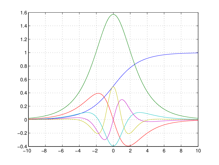
(a) φ⁡(x)\varphi(x) and ρ⁡(x)\rho(x) profiles.
Refer to caption
(b) φ′​(x)\varphi^{\prime}(x) and ρ′​(x)\rho^{\prime}(x) profiles.
Refer to caption
(c) (1−∂x2)φ(x)=2δ0(1-\partial^{2}_{x})\varphi(x)=2\delta_{0} and (1−∂x2)ρ(x)=(1/2)e−2​|x|(1-\partial^{2}_{x})\rho(x)=(1/2)e^{-2|x|} profiles
Figure 1: Variation of peakon and smooth-peakon at initial time with the speed c=1c=1.
Lemma 3.3 (Quadratic Identity; See [5]).

For any u∈L2​(ℝ)u\in L^{2}(\mathbb{R}) and ξ∈ℝ\xi\in\mathbb{R}, it holds

E(u)−E(φc)=∥u−φc(⋅−ξ)∥ℋ2+4c(v(ξ)−c6),E(u)-E(\varphi_{c})=\|u-\varphi_{c}(\cdot-\xi)\|^{2}_{\mathcal{H}}+4c\left(v(\xi)-\frac{c}{6}\right), (3.12)

where v=(4−∂x2)−1uv=(4-\partial^{2}_{x})^{-1}u and c/6=ρc​(0)=maxx∈ℝ⁡ρc​(x−ξ)c/6=\rho_{c}(0)=\max_{x\in\mathbb{R}}\rho_{c}(x-\xi).

Sketch of proof. The proof follows by direct computation, with the aid of two integration by parts, and using that (1−∂x2)φc(⋅−ξ)=2cδξ(1-\partial^{2}_{x})\varphi_{c}(\cdot-\xi)=2c\delta_{\xi}, where δξ\delta_{\xi} denotes the Dirac mass applied at point ξ\xi. □\square

Let u∈H1​(ℝ)u\in H^{1}(\mathbb{R}) with y=(1−∂x2)u∈ℳ+(ℝ)y=(1-\partial^{2}_{x})u\in\mathcal{M}^{+}(\mathbb{R}), and assume that there exists ξ∈ℝ\xi\in\mathbb{R} such that (3.6) holds for some ξ∈ℝ\xi\in\mathbb{R}. We consider now the interval in which the peakon (respectively the smooth-peakon) is concentrated, and we will decompose this interval according to the variation of v=(4−∂x2)−1uv=(4-\partial^{2}_{x})^{-1}u in the following way: we set

α=sup{x<ξ,v⁡(x)=c2400}​and​β=inf{x>ξ,v⁡(x)=c2400}.\alpha=\sup\left\{x<\xi,~v(x)=\frac{c}{2400}\right\}~~\text{and}~~\beta=\inf\left\{x>\xi,~v(x)=\frac{c}{2400}\right\}. (3.13)

According to Lemma 3.2, we know that vv is close to ρc(⋅−ξ)\rho_{c}(\cdot-\xi) in L∞L^{\infty} norm with ρc​(0)=c/6\rho_{c}(0)=c/6. Therefore vv must have at least one local maximum on [α,β][\alpha,\beta]. Assume that on [α,β][\alpha,\beta] the function vv admits k+1k+1 points (ξj)j=1k+1(\xi_{j})_{j=1}^{k+1} with local maximal values for some integer k≥0k\geq 0, where ξ1\xi_{1} is the first local maximum point and ξk+1\xi_{k+1} the last local maximum point22 2 In the case of an infinite countable number of local maximal values, the proof is exactly the same.. Then between ξ1\xi_{1} and ξk+1\xi_{k+1}, the function vv admits kk points (ηj)j=1k(\eta_{j})_{j=1}^{k} with local minimal values. We rename α=η0\alpha=\eta_{0} and β=ηk+1\beta=\eta_{k+1} so that it holds

η0<ξ1<η1<…<ξj<ηj<ξj+1<ηj+1<…<ηk<ξk+1<ηk+1.\eta_{0}<\xi_{1}<\eta_{1}<\ldots<\xi_{j}<\eta_{j}<\xi_{j+1}<\eta_{j+1}<\ldots<\eta_{k}<\xi_{k+1}<\eta_{k+1}. (3.14)

Let

Mj=v(ξj),j=1,…,k+1,andmj=v(ηj),j=1,…,k.M_{j}=v(\xi_{j}),~~j=1,\ldots,k+1,~~\text{and}~~m_{j}=v(\eta_{j}),~~j=1,\ldots,k. (3.15)

By construction

vx(x)≥0,∀x∈[ηj−1,ξj],j=1,…,kv_{x}(x)\geq 0,~~\forall x\in[\eta_{j-1},\xi_{j}],~~j=1,\ldots,k (3.16)

and

vx(x)≤0,∀x∈[ξj,ηj],j=1,…,k+1.v_{x}(x)\leq 0,~~\forall x\in[\xi_{j},\eta_{j}],~~j=1,\ldots,k+1. (3.17)

We claim that

v⁡(x)≤c300,∀x∈ℝ∖[η0,ηk+1],v(x)\leq\frac{c}{300},~~\forall x\in\mathbb{R}\setminus[\eta_{0},\eta_{k+1}], (3.18)
u⁡(x)≤c300,∀x∈ℝ∖[η0,ηk+1],u(x)\leq\frac{c}{300},~~\forall x\in\mathbb{R}\setminus[\eta_{0},\eta_{k+1}], (3.19)

and there exits C0>0C_{0}>0 such that

[η0,ηk+1]⊂[ξ−C0,ξ+C0].[\eta_{0},\eta_{k+1}]\subset[\xi-C_{0},\xi+C_{0}]. (3.20)

Indeed, for some 0<ε≪10<\varepsilon\ll 1 fixed, using (3.11) we have

ρc​(η0−ξ)=v⁡(η0)+O⁡(ε1/4)=c2400+O⁡(ε1/4)≤c350.\rho_{c}(\eta_{0}-\xi)=v(\eta_{0})+O(\varepsilon^{1/4})=\frac{c}{2400}+O(\varepsilon^{1/4})\leq\frac{c}{350}.

Please note that, we abuse notation by writing that the difference between vv and ρc(⋅−ξ)\rho_{c}(\cdot-\xi) is equal to O⁡(ε1/4)O(\varepsilon^{1/4}). Therefore, using that ρc(⋅−ξ)\rho_{c}(\cdot-\xi) is increasing on ]−∞,ξ]]-\infty,\xi], it holds for all x∈]−∞,η0[x\in]-\infty,\eta_{0}[,

v⁡(x)=ρc​(x−ξ)+O⁡(ε1/4)≤c350+O⁡(ε1/4)≤c300.v(x)=\rho_{c}(x-\xi)+O(\varepsilon^{1/4})\leq\frac{c}{350}+O(\varepsilon^{1/4})\leq\frac{c}{300}.

Proceeding in the same way for x∈]ηk+1,+∞[x\in]\eta_{k+1},+\infty[, we obtain (3.18).

One can remark that for all x∈ℝx\in\mathbb{R},

φc​(x)−6​ρc​(x)=c​e−|x|−6​(c3​e−|x|−c6​e−2​|x|)=−c​e−|x|+c​e−2​|x|≤0.\varphi_{c}(x)-6\rho_{c}(x)=ce^{-|x|}-6\left(\frac{c}{3}e^{-|x|}-\frac{c}{6}e^{-2|x|}\right)=-ce^{-|x|}+ce^{-2|x|}\leq 0. (3.21)

Thus, combining (3.10), (3.21) and proceeding as for the estimate (3.18), we infer (3.19).

Finally, from (3.11) we have

ρc​(η0−ξ)=v⁡(η0)+O⁡(ε1/4)=c2400+O⁡(ε1/4)≥c3000.\rho_{c}(\eta_{0}-\xi)=v(\eta_{0})+O(\varepsilon^{1/4})=\frac{c}{2400}+O(\varepsilon^{1/4})\geq\frac{c}{3000}.

Therefore, since ρc=(c/3)e−|⋅|−(c/6)e−2|⋅|\rho_{c}=(c/3)e^{-|\cdot|}-(c/6)e^{-2|\cdot|} and that x↦(1/3)​e−|x|−(1/6)​e−2​|x|x\mapsto(1/3)e^{-|x|}-(1/6)e^{-2|x|} is a positive even function decreasing to 00 on ℝ+\mathbb{R}_{+} (see Fig. 1a), there exists a universal constant C0>0C_{0}>0 such that (3.20) holds.

We now are ready to establish the connection between the conservation laws. Please note that, we will change the order of the extrema of v=(4−∂x2)−1uv=(4-\partial^{2}_{x})^{-1}u while keeping the same notations as in (3.15).

Lemma 3.4 (Connection Between E⁡(⋅)E(\cdot) and the Local Extrema of vv).

Let u∈H1​(ℝ)u\in H^{1}(\mathbb{R}) and v=(4−∂x2)−1u∈H3(ℝ)v=(4-\partial^{2}_{x})^{-1}u\in H^{3}(\mathbb{R}). Define the function gg by

g(x)={2​v+vx​x−3​vx,x<ξ1,2​v+vx​x+3​vx,ξj<x<ηj,2​v+vx​x−3​vx,ηj<x<ξj+1,2​v+vx​x+3​vx,x>ξk+1,j=1,…,k.g(x)=\left\{\begin{aligned} &2v+v_{xx}-3v_{x},~~x<\xi_{1},\\ &2v+v_{xx}+3v_{x},~~\xi_{j}<x<\eta_{j},\\ &2v+v_{xx}-3v_{x},~~\eta_{j}<x<\xi_{j+1},\\ &2v+v_{xx}+3v_{x},~~x>\xi_{k+1},\\ \end{aligned}\right.~~j=1,\ldots,k. (3.22)

Then it holds

∫ℝg2​(x)​𝑑x=E⁡(u)−12​(∑j=0kMj+12−∑j=1kmj2).\int_{\mathbb{R}}g^{2}(x)dx=E(u)-12\left(\sum_{j=0}^{k}M^{2}_{j+1}-\sum_{j=1}^{k}m^{2}_{j}\right). (3.23)

Proof. We have

∫ℝg2​(x)​𝑑x=∫−∞ξ1g2​(x)​𝑑x+∑j=1k∫ξjξj+1g2​(x)​𝑑x+∫ξk+1+∞g2​(x)​𝑑x.\int_{\mathbb{R}}g^{2}(x)dx=\int_{-\infty}^{\xi_{1}}g^{2}(x)dx+\sum_{j=1}^{k}\int_{\xi_{j}}^{\xi_{j+1}}g^{2}(x)dx+\int_{\xi_{k+1}}^{+\infty}g^{2}(x)dx. (3.24)

For j=1,…,kj=1,\ldots,k,

∫ξjξj+1g2​(x)​(x)​𝑑x\displaystyle\int_{\xi_{j}}^{\xi_{j+1}}g^{2}(x)(x)dx =∫ξjηj(2​v+vx​x+3​vx)2+∫ηjξj+1(2​v+vx​x−3​vx)2\displaystyle=\int_{\xi_{j}}^{\eta_{j}}\left(2v+v_{xx}+3v_{x}\right)^{2}+\int_{\eta_{j}}^{\xi_{j+1}}\left(2v+v_{xx}-3v_{x}\right)^{2}
=J+I.\displaystyle=J+I.

Let us compute II,

I\displaystyle I =∫ηjξj+1(4​v2+vx​x2+9​vx2+4​v​vx​x−12​v​vx−6​vx​vx​x)\displaystyle=\int_{\eta_{j}}^{\xi_{j+1}}\left(4v^{2}+v^{2}_{xx}+9v^{2}_{x}+4vv_{xx}-12vv_{x}-6v_{x}v_{xx}\right)
=∫ηjξj+1(4​v2+vx​x2+9​vx2)+4​∫ηjξj+1v​vx​x−12​∫ηjξj+1v​vx−6​∫ηjξj+1vx​vx​x\displaystyle=\int_{\eta_{j}}^{\xi_{j+1}}\left(4v^{2}+v^{2}_{xx}+9v^{2}_{x}\right)+4\int_{\eta_{j}}^{\xi_{j+1}}vv_{xx}-12\int_{\eta_{j}}^{\xi_{j+1}}vv_{x}-6\int_{\eta_{j}}^{\xi_{j+1}}v_{x}v_{xx}
=∫ηjξj+1(4​v2+vx​x2+9​vx2)+I1+I2+I3.\displaystyle=\int_{\eta_{j}}^{\xi_{j+1}}\left(4v^{2}+v^{2}_{xx}+9v^{2}_{x}\right)+I_{1}+I_{2}+I_{3}.

Applying integration by parts and using that vx​(ξj)=vx​(ηj)=0v_{x}(\xi_{j})=v_{x}(\eta_{j})=0, we get

I1=−4∫ηjξj+1vx2,I2=−6∫ηjξj+1∂x(v2)=−6v2(ξj+1)+6v2(ηj)andI3=−3∫ηjξj+1∂x(vx2)=0.I_{1}=-4\int_{\eta_{j}}^{\xi_{j+1}}v^{2}_{x},~~I_{2}=-6\int_{\eta_{j}}^{\xi_{j+1}}\partial_{x}(v^{2})=-6v^{2}(\xi_{j+1})+6v^{2}(\eta_{j})~~\text{and}~~I_{3}=-3\int_{\eta_{j}}^{\xi_{j+1}}\partial_{x}(v^{2}_{x})=0.

Therefore

I=∫ηjξj+1(4​v2+5​vx2+vx​x2)−6​v2​(ξj+1)+6​v2​(ηj).I=\int_{\eta_{j}}^{\xi_{j+1}}\left(4v^{2}+5v^{2}_{x}+v^{2}_{xx}\right)-6v^{2}(\xi_{j+1})+6v^{2}(\eta_{j}). (3.25)

Similar computations lead to

J=∫ξjηj(4​v2+5​vx2+vx​x2)−6​v2​(ξj)+6​v2​(ηj),∫−∞ξ1g2​(x)​𝑑x=∫−∞ξ1(4​v2+5​vx2+vx​x2)−6​v2​(ξ1)J=\int_{\xi_{j}}^{\eta_{j}}\left(4v^{2}+5v^{2}_{x}+v^{2}_{xx}\right)-6v^{2}(\xi_{j})+6v^{2}(\eta_{j}),~~\int_{-\infty}^{\xi_{1}}g^{2}(x)\,dx=\int_{-\infty}^{\xi_{1}}\left(4v^{2}+5v^{2}_{x}+v^{2}_{xx}\right)-6v^{2}(\xi_{1}) (3.26)

and

∫ξk+1+∞g2​(x)​𝑑x=∫ξk+1+∞(4​v2+5​vx2+vx​x2)−6​v2​(ξk+1).\int_{\xi_{k+1}}^{+\infty}g^{2}(x)\,dx=\int_{\xi_{k+1}}^{+\infty}\left(4v^{2}+5v^{2}_{x}+v^{2}_{xx}\right)-6v^{2}(\xi_{k+1}). (3.27)

Adding II and JJ, and summing over j∈{1,…,k}j\in\{1,\ldots,k\}, we obtain

∫ξ1ξk+1g2​(x)​𝑑x=∫ξ1ξk+1(4​v2+5​vx2+vx​x2)−6​∑j=1kv2​(ξj+1)−6​∑j=1kv2​(ξj)+12​∑j=1kv2​(ηj).\int_{\xi_{1}}^{\xi_{k+1}}g^{2}(x)dx=\int_{\xi_{1}}^{\xi_{k+1}}\left(4v^{2}+5v^{2}_{x}+v^{2}_{xx}\right)-6\sum_{j=1}^{k}v^{2}(\xi_{j+1})-6\sum_{j=1}^{k}v^{2}(\xi_{j})+12\sum_{j=1}^{k}v^{2}(\eta_{j}). (3.28)

The lemma follows by combining (3.24) and (3.26)-(3.28). □\square

Lemma 3.5 (Connection Between F⁡(⋅)F(\cdot) and the Local Extrema of vv).

Let u∈H1​(ℝ)u\in H^{1}(\mathbb{R}) and v=(4−∂x2)−1u∈H3(ℝ)v=(4-\partial^{2}_{x})^{-1}u\in H^{3}(\mathbb{R}). Define the function hh by

h(x)={−vx​x−6​vx+16​v,x<ξ1,−vx​x+6​vx+16​v,ξj<x<ηj,−vx​x−6​vx+16​v,ηj<x<ξj+1,−vx​x+6​vx+16​v,x>ξk+1,j=1,…,k.h(x)=\left\{\begin{aligned} &-v_{xx}-6v_{x}+16v,~~x<\xi_{1},\\ &-v_{xx}+6v_{x}+16v,~~\xi_{j}<x<\eta_{j},\\ &-v_{xx}-6v_{x}+16v,~~\eta_{j}<x<\xi_{j+1},\\ &-v_{xx}+6v_{x}+16v,~~x>\xi_{k+1},\\ \end{aligned}\right.~~j=1,\ldots,k. (3.29)

Then it holds

∫ℝh⁡(x)​g2​(x)​𝑑x=F⁡(u)−144​(∑j=0kMj+13−∑j=1kmj3).\int_{\mathbb{R}}h(x)g^{2}(x)dx=F(u)-144\left(\sum_{j=0}^{k}M^{3}_{j+1}-\sum_{j=1}^{k}m^{3}_{j}\right). (3.30)

Proof. We have

∫ℝh⁡(x)​g2​(x)​𝑑x=∫−∞ξ1h⁡(x)​g2​(x)​𝑑x+∑j=1k∫ξjξj+1h⁡(x)​g2​(x)​𝑑x+∫ξk+1+∞h⁡(x)​g2​(x)​𝑑x.\int_{\mathbb{R}}h(x)g^{2}(x)dx=\int_{-\infty}^{\xi_{1}}h(x)g^{2}(x)dx+\sum_{j=1}^{k}\int_{\xi_{j}}^{\xi_{j+1}}h(x)g^{2}(x)dx+\int_{\xi_{k+1}}^{+\infty}h(x)g^{2}(x)dx. (3.31)

For j=1,…,kj=1,\ldots,k,

∫ξjξj+1h⁡(x)​g2​(x)​𝑑x\displaystyle\int_{\xi_{j}}^{\xi_{j+1}}h(x)g^{2}(x)dx =∫ξjηj(−vx​x−6​vx+16​v)​(2​v+vx​x−3​vx)2\displaystyle=\int_{\xi_{j}}^{\eta_{j}}\left(-v_{xx}-6v_{x}+16v\right)\left(2v+v_{xx}-3v_{x}\right)^{2}
+∫ηjξj+1(−vx​x+6vx+16v)(2v+vx​x+3vx)2\displaystyle\hskip 28.45274pt+\int_{\eta_{j}}^{\xi_{j+1}}\left(-v_{xx}+6v_{x}+16v\right)\left(2v+v_{xx}+3v_{x}\right)^{2}
=J+I.\displaystyle=J+I.

Let us compute II,

I\displaystyle I =∫ηjξj+1(−vx​x3+12​v​vx​x2+64​v3+60​v2​vx​x)−54​∫ηjξj+1vx3+27​∫ηjξj+1vx2​vx​x\displaystyle=\int_{\eta_{j}}^{\xi_{j+1}}\left(-v^{3}_{xx}+12vv^{2}_{xx}+64v^{3}+60v^{2}v_{xx}\right)-54\int_{\eta_{j}}^{\xi_{j+1}}v^{3}_{x}+27\int_{\eta_{j}}^{\xi_{j+1}}v^{2}_{x}v_{xx}
−108∫ηjξj+1vvxvx​x−216∫ηjξj+1v2vx+216∫ηjξj+1vv2x\displaystyle\hskip 28.45274pt-108\int_{\eta_{j}}^{\xi_{j+1}}vv_{x}v_{xx}-216\int_{\eta_{j}}^{\xi_{j+1}}v^{2}v_{x}+216\int_{\eta_{j}}^{\xi_{j+1}}vv^{2}_{x}
=∫ηjξj+1(−vx​x3+12​v​vx​x2+64​v3+60​v2​vx​x)\displaystyle=\int_{\eta_{j}}^{\xi_{j+1}}\left(-v^{3}_{xx}+12vv^{2}_{xx}+64v^{3}+60v^{2}v_{xx}\right)
−54∫ηjξj+1v3x+I1+I2+I3+I4.\displaystyle\hskip 28.45274pt-54\int_{\eta_{j}}^{\xi_{j+1}}v^{3}_{x}+I_{1}+I_{2}+I_{3}+I_{4}.

Applying integration by parts and using that vx​(ξj)=vx​(ηj)=0v_{x}(\xi_{j})=v_{x}(\eta_{j})=0, we get

I1=9∫ηjξj+1∂x(vx3)=0,I2=54∫ηjξj+1vx3,I3=−72∫ηjξj+1∂x(v3)=−72v3(ξj+1)+72v3(ηj)I_{1}=9\int_{\eta_{j}}^{\xi_{j+1}}\partial_{x}(v^{3}_{x})=0,~~I_{2}=54\int_{\eta_{j}}^{\xi_{j+1}}v^{3}_{x},~~I_{3}=-72\int_{\eta_{j}}^{\xi_{j+1}}\partial_{x}(v^{3})=-72v^{3}(\xi_{j+1})+72v^{3}(\eta_{j})

and

I4\displaystyle I_{4} =108∫ηjξj+1∂x(v2)vx=−108∫ηjξj+1v2vx​x.\displaystyle=108\int_{\eta_{j}}^{\xi_{j+1}}\partial_{x}(v^{2})v_{x}=-108\int_{\eta_{j}}^{\xi_{j+1}}v^{2}v_{xx}.

Therefore

I=∫ηjξj+1(−vx​x3+12​v​vx​x2+64​v3+60​v2​vx​x)−72​v3​(ξj+1)+72​v3​(ηj).I=\int_{\eta_{j}}^{\xi_{j+1}}\left(-v^{3}_{xx}+12vv^{2}_{xx}+64v^{3}+60v^{2}v_{xx}\right)-72v^{3}(\xi_{j+1})+72v^{3}(\eta_{j}). (3.32)

Similar computations lead to

J=∫ξjηj(−vx3+12​v​vx​x2+64​v3+60​v2​vx​x)−72​v3​(ξj)+72​v3​(ηj),J=\int_{\xi_{j}}^{\eta_{j}}\left(-v^{3}_{x}+12vv^{2}_{xx}+64v^{3}+60v^{2}v_{xx}\right)-72v^{3}(\xi_{j})+72v^{3}(\eta_{j}), (3.33)
∫−∞ξ1h⁡(x)​g2​(x)​𝑑x=∫−∞ξ1(−vx3+12​v​vx​x2+64​v3+60​v2​vx​x)−72​v3​(ξ1)\int_{-\infty}^{\xi_{1}}h(x)g^{2}(x)\\ dx=\int_{-\infty}^{\xi_{1}}\left(-v^{3}_{x}+12vv^{2}_{xx}+64v^{3}+60v^{2}v_{xx}\right)-72v^{3}(\xi_{1}) (3.34)

and

∫ξk+1+∞h⁡(x)​g2​(x)​𝑑x=∫ξk+1+∞(−vx3+12​v​vx​x2+64​v3+60​v2​vx​x)−72​v3​(ξk+1).\int_{\xi_{k+1}}^{+\infty}h(x)g^{2}(x)\,dx=\int_{\xi_{k+1}}^{+\infty}\left(-v^{3}_{x}+12vv^{2}_{xx}+64v^{3}+60v^{2}v_{xx}\right)-72v^{3}(\xi_{k+1}). (3.35)

Adding (3.25) and (3.33), and summing over j∈{1,…,k}j\in\{1,\ldots,k\}, we obtain

∫ξ1ξk+1h⁡(x)​g2​(x)​𝑑x\displaystyle\int_{\xi_{1}}^{\xi_{k+1}}h(x)g^{2}(x)dx =∫ξ1ξk+1(−vx3+12​v​vx​x2+64​v3+60​v2​vx​x)−72​∑j=1kv3​(ξj+1)\displaystyle=\int_{\xi_{1}}^{\xi_{k+1}}\left(-v^{3}_{x}+12vv^{2}_{xx}+64v^{3}+60v^{2}v_{xx}\right)-72\sum_{j=1}^{k}v^{3}(\xi_{j+1})
−72∑j=1kv3(ξj)+72∑j=1kv3(ηj).\displaystyle\hskip 28.45274pt-72\sum_{j=1}^{k}v^{3}(\xi_{j})+72\sum_{j=1}^{k}v^{3}(\eta_{j}). (3.36)

The lemma follows by combining (3.31) and (3.34)-(3.36). □\square

Lemma 3.6 (Connection Between E⁡(⋅)E(\cdot) and F⁡(⋅)F(\cdot)).

Let u∈H1​(ℝ)u\in H^{1}(\mathbb{R}), with y=(1−∂x2)u∈ℳ+(ℝ)y=(1-\partial^{2}_{x})u\in{\mathcal{M}}^{+}({\mathbb{R}}), that satisfies (3.6) for some ξ∈ℝ\xi\in\mathbb{R}. Assume that v=(4−∂x2)−1uv=(4-\partial^{2}_{x})^{-1}u satisfies (3.13)-(3.20), with local extrema on [η0,ηk+1][\eta_{0},\eta_{k+1}] arranged in decreasing order in the following way:

M1≥M2≥…≥Mk+1≥0,m1≥m2≥…≥mk≥0,Mj+1≥mj,j=1,…,k.M_{1}\geq M_{2}\geq\ldots\geq M_{k+1}\geq 0,~~m_{1}\geq m_{2}\geq\ldots\geq m_{k}\geq 0,~~M_{j+1}\geq m_{j},~j=1,\ldots,k. (3.37)

There exists ε0>0\varepsilon_{0}>0 only depending on the speed cc, such that if 0<ε<ε00<\varepsilon<\varepsilon_{0}, then it holds

M13−14​E​(u)​M1+172​F​(u)≤0.M^{3}_{1}-\frac{1}{4}E(u)M_{1}+\frac{1}{72}F(u)\leq 0. (3.38)

Proof. The key is to show that h≤18​M1h\leq 18M_{1} on ℝ\mathbb{R}. Note that by (3.6) we know that 18​M1≥c/418M_{1}\geq c/4. We rewrite the function hh as

h(x)={−vx​x−6​vx+16​v,x<η0,−(∂2x+3∂x+2)v−3vx+18v,η0<x<ξ1,−(∂2x−3∂x+2)v+3vx+18v,ξj<x<ηj,−(∂2x+3∂x+2)v−3vx+18v,ηj<x<ξj+1,−(∂2x−3∂x+2)v+3vx+18v,ξk+1<x<ηk+1,−vx​x+6​vx+16​v,x>ηk+1,j=1,…,k.h(x)=\left\{\begin{aligned} &-v_{xx}-6v_{x}+16v,~~x<\eta_{0},\\ &-\left(\partial^{2}_{x}+3\partial_{x}+2\right)v-3v_{x}+18v,~~\eta_{0}<x<\xi_{1},\\ &-\left(\partial^{2}_{x}-3\partial_{x}+2\right)v+3v_{x}+18v,~~\xi_{j}<x<\eta_{j},\\ &-\left(\partial^{2}_{x}+3\partial_{x}+2\right)v-3v_{x}+18v,~~\eta_{j}<x<\xi_{j+1},\\ &-\left(\partial^{2}_{x}-3\partial_{x}+2\right)v+3v_{x}+18v,~~\xi_{k+1}<x<\eta_{k+1},\\ &-v_{xx}+6v_{x}+16v,~~x>\eta_{k+1},\\ \end{aligned}\right.~~j=1,\ldots,k.

First, one can remark that for all x∈ℝx\in\mathbb{R},

v⁡(x)=e−2​x4​∫−∞xe2​x′​u​(x′)​d​x′+e2​x4​∫x+∞e−2​x′​u​(x′)​d​x′v(x)=\frac{e^{-2x}}{4}\int_{-\infty}^{x}e^{2x^{\prime}}u(x^{\prime})dx^{\prime}+\frac{e^{2x}}{4}\int_{x}^{+\infty}e^{-2x^{\prime}}u(x^{\prime})dx^{\prime}

and

vx(x)=−e−2​x2∫−∞xe2​x′u(x′)dx′+e2​x2∫x+∞e−2​x′u(x′)dx′.v_{x}(x)=-\frac{e^{-2x}}{2}\int_{-\infty}^{x}e^{2x^{\prime}}u(x^{\prime})dx^{\prime}+\frac{e^{2x}}{2}\int_{x}^{+\infty}e^{-2x^{\prime}}u(x^{\prime})dx^{\prime}.

Then using that u=(1−∂x2)−1y≥0u=(1-\partial^{2}_{x})^{-1}y\geq 0 on ℝ\mathbb{R}, we get

|vx​(x)|≤2​v​(x),∀x∈ℝ.|v_{x}(x)|\leq 2v(x),~~\forall x\in\mathbb{R}. (3.39)

Next, if x∈ℝ∖[η0,ηk+1]x\in\mathbb{R}\setminus[\eta_{0},\eta_{k+1}], using that vx​x=4​v−uv_{xx}=4v-u, (3.18), (3.19) and (3.39), it holds

h\displaystyle h ≤|vx​x|+6​|vx|+16​v≤u+32​v≤c9.\displaystyle\leq|v_{xx}|+6|v_{x}|+16v\leq u+32v\leq\frac{c}{9}.

If η0<x<ξ1\eta_{0}<x<\xi_{1}, then vx≥0v_{x}\geq 0, and using that y=(1−∂x2)u≥0y=(1-\partial^{2}_{x})u\geq 0, it follows from Lemma 2.2 that

h\displaystyle h =−(∂x2+3∂x+2)v−3vx+18v\displaystyle=-(\partial^{2}_{x}+3\partial_{x}+2)v-3v_{x}+18v
=−(2+∂x)(4−∂x2)−1(1+∂x)u−3vx+18v\displaystyle=-(2+\partial_{x})(4-\partial^{2}_{x})^{-1}(1+\partial_{x})u-3v_{x}+18v
≤18​v.\displaystyle\leq 18v.

If ξj<x<ηj\xi_{j}<x<\eta_{j}, then vx≤0v_{x}\leq 0, and similarly using that y=(1−∂x2)u≥0y=(1-\partial^{2}_{x})u\geq 0, it follows from Lemma 2.2 that

h\displaystyle h =−(∂x2−3∂x+2)v+3vx+18v\displaystyle=-(\partial^{2}_{x}-3\partial_{x}+2)v+3v_{x}+18v
=−(2−∂x)(4−∂x2)−1(1−∂x)u+3vx+18v\displaystyle=-(2-\partial_{x})(4-\partial^{2}_{x})^{-1}(1-\partial_{x})u+3v_{x}+18v
≤18​v.\displaystyle\leq 18v.

Therefore, it holds

h⁡(x)≤18​maxx∈ℝ⁡v⁡(x)=18​M1,∀x∈ℝ.h(x)\leq 18\max_{x\in\mathbb{R}}v(x)=18M_{1},~~\forall x\in\mathbb{R}. (3.40)

Now, combining (3.23), (3.30) and (3.40), we get

F⁡(u)−144\displaystyle F(u)-144 (∑j=0kMj+13−∑j=1kmj3)\displaystyle\left(\sum_{j=0}^{k}M^{3}_{j+1}-\sum_{j=1}^{k}m^{3}_{j}\right)
=∫ℝh⁡(x)​g2​(x)​𝑑x\displaystyle=\int_{\mathbb{R}}h(x)g^{2}(x)dx
≤‖h‖L∞​(ℝ)​∫ℝg2​(x)​𝑑x\displaystyle\leq\|h\|_{L^{\infty}(\mathbb{R})}\int_{\mathbb{R}}g^{2}(x)dx
≤18​M1​[E⁡(u)−12​(∑j=0kMj+12−∑j=1kmj2)].\displaystyle\leq 18M_{1}\left[E(u)-12\left(\sum_{j=0}^{k}M^{2}_{j+1}-\sum_{j=1}^{k}m^{2}_{j}\right)\right].

For j=1,…,kj=1,\ldots,k, we set

Aj=Mj+13−mj3​and​Bj=Mj+12−mj2,A_{j}=M^{3}_{j+1}-m^{3}_{j}~~\text{and}~~B_{j}=M^{2}_{j+1}-m^{2}_{j},

and our inequality becomes

M13−14​E​(u)​M1+172​F​(u)≤2​∑j=1k(Aj−32​M1​Bj).M^{3}_{1}-\frac{1}{4}E(u)M_{1}+\frac{1}{72}F(u)\leq 2\sum_{j=1}^{k}\left(A_{j}-\frac{3}{2}M_{1}B_{j}\right). (3.41)

On the other hand, using that Mj+1≥mjM_{j+1}\geq m_{j}, we have

Aj−32​M1​Bj=−12​(Mj+1−mj)​(3​M1​mj+3​M1​Mj+1−2​Mj+1​mj−2​Mj+12−2​mj2)≤0.A_{j}-\frac{3}{2}M_{1}B_{j}=-\frac{1}{2}\left(M_{j+1}-m_{j}\right)\left(3M_{1}m_{j}+3M_{1}M_{j+1}-2M_{j+1}m_{j}-2M^{2}_{j+1}-2m^{2}_{j}\right)\leq 0. (3.42)

Finally, combining (3.41) and (3.42), we obtain the lemma. □\square

Proof of Theorem 3.1. We argue as El Dika and Molinet in [3]. As noticed after the statement of the theorem, it suffices to prove (3.7) assuming that u∈H1​(ℝ)u\in H^{1}(\mathbb{R}) satisfies (3.1), (3.2) and (3.4)-(3.6). We set M1=v⁡(ξ1)=maxx∈ℝ⁡v⁡(x)M_{1}=v(\xi_{1})=\max_{x\in\mathbb{R}}v(x) and δ=c/6−M1\delta=c/6-M_{1}. We first remark that if δ≤0\delta\leq 0, combining (3.4) and (3.12), it holds

∥u−φc(⋅−ξ1)∥ℋ≤|E(u0)−E(φc)|1/2≤O(ε),\|u-\varphi_{c}(\cdot-\xi_{1})\|_{\mathcal{H}}\leq|E(u_{0})-E(\varphi_{c})|^{1/2}\leq O(\varepsilon),

that yields the desired result. Now suppose that δ>0\delta>0, that is the maximum of the function vv is less than the maximum of ρc\rho_{c}. Combining (3.4), (3.5) and (3.38), we get

M13−14​E​(φc)​M1+172​F​(φc)≤O⁡(ε2).M^{3}_{1}-\frac{1}{4}E(\varphi_{c})M_{1}+\frac{1}{72}F(\varphi_{c})\leq O(\varepsilon^{2}).

Using that E⁡(φc)=c2/3E(\varphi_{c})=c^{2}/3 and F⁡(φc)=2​c3/3F(\varphi_{c})=2c^{3}/3, our inequality becomes

(M1−c6)2​(M1+c3)≤O⁡(ε2).\left(M_{1}-\frac{c}{6}\right)^{2}\left(M_{1}+\frac{c}{3}\right)\leq O(\varepsilon^{2}).

Substituting M1M_{1} by c/6−δc/6-\delta and using that (M1+c/3)−1<3/c(M_{1}+c/3)^{-1}<3/c, it holds

δ2≤O⁡(ε2)⇒δ≤O⁡(ε).\delta^{2}\leq O(\varepsilon^{2})\Rightarrow\delta\leq O(\varepsilon). (3.43)

Finally, combining (3.4), (3.12) and (3.43), we obtain

∥u−φc(⋅−ξ1)∥ℋ≤Cε,\|u-\varphi_{c}(\cdot-\xi_{1})\|_{\mathcal{H}}\leq C\sqrt{\varepsilon},

where C>0C>0 only depends on the speed cc. This completes the proof of the stability of a single peakon.

4 Stability of the trains of peakons

For γ>0\gamma>0 and L>0L>0, we define the following neighborhood of all the sums of NN peakons of speed c1,…,cNc_{1},...,c_{N} with spatial shifts ziz_{i} that satisfied zi−zi−1≥Lz_{i}-z_{i-1}\geq L,

U(γ,L)={u∈H1(ℝ);infzi−zi−1>L‖u−∑i=1Nφci(⋅−zi)‖ℋ≤γ}.U(\gamma,L)=\left\{u\in H^{1}(\mathbb{R});~\inf_{z_{i}-z_{i-1}>L}\left\|u-\sum_{i=1}^{N}\varphi_{c_{i}}(\cdot-z_{i})\right\|_{\mathcal{H}}\leq\gamma\right\}. (4.1)

By the continuity of the map t↦u⁡(t)t\mapsto u(t) from [0,T[[0,T[ into H1​(ℝ)↪ℋH^{1}(\mathbb{R})\hookrightarrow\mathcal{H}, to prove Theorem 1.11.1 it suffices to prove that there exist A>0A>0, ε0>0\varepsilon_{0}>0 and L0>0L_{0}>0 such that for all L>L0L>L_{0} and 0<ε<ε00<\varepsilon<\varepsilon_{0}, if u0u_{0} satisfies (1.12)-(1.14), and if for some 0<t0<T0<t_{0}<T,

u(t)∈U(A(ε+L−1/8),L2),∀t∈[0,t0],u(t)\in U\left(A(\sqrt{\varepsilon}+L^{-1/8}),\frac{L}{2}\right),~~\forall t\in[0,t_{0}], (4.2)

then

u(t0)∈U(A2(ε+L−1/8),2​L3).u(t_{0})\in U\left(\frac{A}{2}(\sqrt{\varepsilon}+L^{-1/8}),\frac{2L}{3}\right). (4.3)

Therefore, in the sequel of this section we will assume (4.2) for some 0<ε<ε00<\varepsilon<\varepsilon_{0} and L>L0L>L_{0}, with AA, ε0\varepsilon_{0} and L0L_{0} to be specified later, and we will prove (4.3).

Remark 4.1 (Distance Between vv and the Sum of NN Smooth-peakons).

From the definition of E⁡(⋅)E(\cdot) and ℋ\mathcal{H} (see respectively (1.3) and (1.6)), one can clearly see that ‖u‖ℋ\|u\|_{\mathcal{H}} is equivalent to ‖v‖H2​(ℝ)\|v\|_{H^{2}(\mathbb{R})}, where v=(4−∂x2)−1uv=(4-\partial^{2}_{x})^{-1}u. Let t1∈[0,t0]t_{1}\in[0,t_{0}] fixed, if u⁡(t1)∈U⁡(γ,L/2)u(t_{1})\in U(\gamma,L/2), then there exists Z~=(z~i)i=1N\tilde{Z}=(\tilde{z}_{i})_{i=1}^{N} with z~i−z~i−1≥L/2\tilde{z}_{i}-\tilde{z}_{i-1}\geq L/2, such that v⁡(t1)∈H3​(ℝ)↪C2​(ℝ)v(t_{1})\in H^{3}(\mathbb{R})\hookrightarrow C^{2}(\mathbb{R}) stays close to ∑i=1Nρci(⋅−z~i)\sum_{i=1}^{N}\rho_{c_{i}}(\cdot-\tilde{z}_{i}) in the H2H^{2} norm, where ρci\rho_{c_{i}} is defined in (3.8).

4.1 Control of the distance between the peakons

In this subsection, we want to prove that the different bumps of uu (respectively of vv) that are individually close to a peakon (respectively a smooth-peakon) get away from each others as time is increasing. This is crucial in our analysis since we do not know how to manage strong interactions.

Lemma 4.1 (Decomposition of the Solution Around φc\varphi_{c}).

Let u0u_{0} satisfying (1.12)-(1.14). There exist γ0>0\gamma_{0}>0, L0>0L_{0}>0 and C0>0C_{0}>0 such that for all 0<γ<γ00<\gamma<\gamma_{0} and 0<L0<L0<L_{0}<L, if u⁡(t)∈U⁡(γ,L/2)u(t)\in U(\gamma,L/2) on [0,t0][0,t_{0}] for some 0<t0<T0<t_{0}<T, then there exist N​C1N~C^{1} functions x~1,…,x~N\tilde{x}_{1},\ldots,\tilde{x}_{N} defined on [0,t0][0,t_{0}] such that

‖u(t)−∑i=1Nφci(⋅−x~i(t))‖ℋ≤O(γ),\left\|u(t)-\sum_{i=1}^{N}\varphi_{c_{i}}(\cdot-\tilde{x}_{i}(t))\right\|_{\mathcal{H}}\leq O(\gamma), (4.4)
‖v(t)−∑i=1Nρci(⋅−x~i(t))‖C1​(ℝ)≤O(γ),\left\|v(t)-\sum_{i=1}^{N}\rho_{c_{i}}(\cdot-\tilde{x}_{i}(t))\right\|_{C^{1}(\mathbb{R})}\leq O(\gamma), (4.5)
|x~˙i(t)−ci|≤c1−2(O(γ)+O(e−L/4)),i=1,…,N,\left|\dot{\tilde{x}}_{i}(t)-c_{i}\right|\leq c_{1}^{-2}\left(O(\gamma)+O(e^{-L/4})\right),~~i=1,\ldots,N, (4.6)

and

x~i(t)−x~i−1(t)≥3​L4+(ci−ci−1)​t2,i=2,…,N.\tilde{x}_{i}(t)-\tilde{x}_{i-1}(t)\geq\frac{3L}{4}+\frac{(c_{i}-c_{i-1})t}{2},~~i=2,\ldots,N. (4.7)

Moreover, for i=1,…,Ni=1,\ldots,N, setting Ji=[yi​(t),yi+1​(t)]J_{i}=[y_{i}(t),y_{i+1}(t)], with

{y1=−∞,yi​(t)=x~i−1​(t)+x~i​(t)2,yN+1=+∞,i=2,…,N,\left\{\begin{aligned} &y_{1}=-\infty,\\ &y_{i}(t)=\frac{\tilde{x}_{i-1}(t)+\tilde{x}_{i}(t)}{2},\\ &y_{N+1}=+\infty,\\ \end{aligned}\right.~~i=2,\ldots,N, (4.8)

it holds

|ξ1i(t)−x~i(t)|≤L12,i=1,…,N,\left|\xi^{i}_{1}(t)-\tilde{x}_{i}(t)\right|\leq\frac{L}{12},~~i=1,\ldots,N, (4.9)

where ξ11​(t),…,ξ1N​(t)\xi^{1}_{1}(t),\ldots,\xi^{N}_{1}(t) are any point such that

v(t,ξ1i(t))=maxx∈Jiv(t,x),i=1,…,N,v\left(t,\xi^{i}_{1}(t)\right)=\max_{x\in J_{i}}v(t,x),~~i=1,\ldots,N, (4.10)

and where v=(4−∂x2)−1uv=(4-\partial^{2}_{x})^{-1}u and O⁡(⋅)O(\cdot) only depends on the speeds (ci)i=1N(c_{i})_{i=1}^{N}.

Proof. We will slightly modify the construction done by El Dika and Molinet in [3]. One can remark that the peakons φci(⋅−cit)\varphi_{c_{i}}(\cdot-c_{i}t) and the smooth-peakons ρci(⋅−cit)\rho_{c_{i}}(\cdot-c_{i}t) travel at the same speed cic_{i}, thanks to this, we will do our construction with v=(4−∂x2)−1uv=(4-\partial^{2}_{x})^{-1}u instead of uu. We do that because the ℋ\mathcal{H} (equivalent to L2L^{2}) approximation (4.2) does not permit us to construct a C1C^{1} function, which is crucial for application of the Implicit Function Theorem. We note that the same approach can also be used for the CH equation.

For Z=(z1,…,zN)∈ℝNZ=(z_{1},\ldots,z_{N})\in\mathbb{R}^{N} fixed such that |zi−zi−1|>L/2|z_{i}-z_{i-1}|>L/2, we set

RZ(⋅)=∑i=1Nρci(⋅−zi)andSZ(⋅)=∑i=1Nφci(⋅−zi).R_{Z}(\cdot)=\sum_{i=1}^{N}\rho_{c_{i}}(\cdot-z_{i})~~\text{and}~~S_{Z}(\cdot)=\sum_{i=1}^{N}\varphi_{c_{i}}(\cdot-z_{i}). (4.11)

For 0<γ<γ00<\gamma<\gamma_{0}, we define the function

𝒴:(−γ,γ)N\displaystyle\mathcal{Y}:(-\gamma,\gamma)^{N} ×BH2​(RZ,γ)→ℝN,\displaystyle\times B_{H^{2}}(R_{Z},\gamma)\rightarrow\mathbb{R}^{N},
(y1,…,yN,v)↦(𝒴1​(y1,…,yN,v),…,𝒴N​(y1,…,yN,v))\displaystyle(y_{1},\ldots,y_{N},v)\mapsto\left(\mathcal{Y}^{1}(y_{1},\ldots,y_{N},v),\ldots,\mathcal{Y}^{N}(y_{1},\ldots,y_{N},v)\right)

with

𝒴i(y1,…,yN,v)=∫ℝ(v−∑j=1Nρcj(⋅−zj−yj))∂xρci(⋅−zi−yi).\mathcal{Y}^{i}(y_{1},\ldots,y_{N},v)=\int_{\mathbb{R}}\left(v-\sum_{j=1}^{N}\rho_{c_{j}}(\cdot-z_{j}-y_{j})\right)\partial_{x}\rho_{c_{i}}(\cdot-z_{i}-y_{i}).

YY is clearly of class C1C^{1}. For i=1,…,Ni=1,\ldots,N,

∂𝒴i∂yi(y1,…,yN,v)=−∫ℝ(v−∑1≤j≤Nj≠iρcj(⋅−zj−yj))∂x2ρci(⋅−zi−yi)\frac{\partial\mathcal{Y}^{i}}{\partial y_{i}}(y_{1},\ldots,y_{N},v)=-\int_{\mathbb{R}}\left(v-\sum\limits_{\underset{j\neq i}{1\leq j\leq N}}\rho_{c_{j}}(\cdot-z_{j}-y_{j})\right)\partial^{2}_{x}\rho_{c_{i}}(\cdot-z_{i}-y_{i})

and for j≠ij\neq i,

∂𝒴i∂yj(y1,…,yN,v)=∫ℝ∂xρcj(⋅−zj−yj)∂xρci(⋅−zi−yi).\frac{\partial\mathcal{Y}^{i}}{\partial y_{j}}(y_{1},\ldots,y_{N},v)=\int_{\mathbb{R}}\partial_{x}\rho_{c_{j}}(\cdot-z_{j}-y_{j})\partial_{x}\rho_{c_{i}}(\cdot-z_{i}-y_{i}).

Hence

∂𝒴i∂yi​(0,…,0,RZ)=‖∂xρci‖L2​(ℝ)2=ci254≥c1254\frac{\partial\mathcal{Y}^{i}}{\partial y_{i}}(0,\ldots,0,R_{Z})=\|\partial_{x}\rho_{c_{i}}\|^{2}_{L^{2}(\mathbb{R})}=\frac{c^{2}_{i}}{54}\geq\frac{c^{2}_{1}}{54}

and for j≠ij\neq i, using the exponential decay of φci\varphi_{c_{i}} and that |zi−zi−1|>L/2|z_{i}-z_{i-1}|>L/2, for L>L0>0L>L_{0}>0 with L0≫1L_{0}\gg 1, it holds

|∂𝒴i∂yj​(0,…,0,RZ)|\displaystyle\left|\frac{\partial\mathcal{Y}^{i}}{\partial y_{j}}(0,\ldots,0,R_{Z})\right|
=|∫ℝ∂xρcj,α(⋅−zj)∂xρci,α(⋅−zi)|\displaystyle\hskip 28.45274pt=\left|\int_{\mathbb{R}}\partial_{x}\rho_{c_{j},\alpha}(\cdot-z_{j})\partial_{x}\rho_{c_{i},\alpha}(\cdot-z_{i})\right|
=|∫ℝρcj,α(⋅−zj)∂x2ρci,α(⋅−zi)|\displaystyle\hskip 28.45274pt=\left|\int_{\mathbb{R}}\rho_{c_{j},\alpha}(\cdot-z_{j})\partial^{2}_{x}\rho_{c_{i},\alpha}(\cdot-z_{i})\right|
≤19(ci−α)(cj−α){∫ℝe−|x−zj|−|x−zi|dx+2∫ℝe−|x−zj|−2​|x−zi|dx\displaystyle\hskip 28.45274pt\leq\frac{1}{9}(c_{i}-\alpha)(c_{j}-\alpha)\left\{\int_{\mathbb{R}}e^{-|x-z_{j}|-|x-z_{i}|}dx+2\int_{\mathbb{R}}e^{-|x-z_{j}|-2|x-z_{i}|}dx\right.
+12∫ℝe−2​|x−zj|−|x−zi|dx+∫ℝe−2​|x−zj|−2​|x−zi|dx}\displaystyle\hskip 56.9055pt\left.+\frac{1}{2}\int_{\mathbb{R}}e^{-2|x-z_{j}|-|x-z_{i}|}dx+\int_{\mathbb{R}}e^{-2|x-z_{j}|-2|x-z_{i}|}dx\right\}
≤O(e−L/4).\displaystyle\hskip 28.45274pt\leq O(e^{-L/4}).

We deduce that, for L>0L>0 large enough, D(y1,…,yN)​𝒴​(0,…,0,RZ)=D+PD_{(y_{1},\ldots,y_{N})}\mathcal{Y}(0,\ldots,0,R_{Z})=D+P where DD is an invertible diagonal matrix with ‖D−1‖≤(c1/3​6)−2\|D^{-1}\|\leq(c_{1}/3\sqrt{6})^{-2} and ∥P∥≤O(e−L/4)\|P\|\leq O(e^{-L/4}). Hence there exists L0>0L_{0}>0 such that for L>L0L>L_{0}, D(y1,…,yN)​𝒴​(0,…,0,RZ)D_{(y_{1},\ldots,y_{N})}\mathcal{Y}(0,\ldots,0,R_{Z}) is invertible with an inverse matrix of norm smaller than 2​(c1/3​6)−22(c_{1}/3\sqrt{6})^{-2}. From the Implicit Function Theorem we deduce that there exists β0>0\beta_{0}>0 and C1C^{1} functions (y1,…,yN)(y_{1},\ldots,y_{N}) from BH2​(RZ,β0)B_{H^{2}}(R_{Z},\beta_{0}) to a neighborhood of (0,…,0)(0,\ldots,0) which are uniquely determined such that

𝒴⁡(y1​(v),…,yN​(v),v)=0,∀v∈BH2​(RZ,β0).\mathcal{Y}(y_{1}(v),\ldots,y_{N}(v),v)=0,~~\forall v\in B_{H^{2}}(R_{Z},\beta_{0}).

In particular, there exists C0>0C_{0}>0 such that if v∈BH2​(RZ,β)v\in B_{H^{2}}(R_{Z},\beta), with 0<β≤β00<\beta\leq\beta_{0}, then

∑i=1N|yi​(v)|≤C0​β.\sum_{i=1}^{N}|y_{i}(v)|\leq C_{0}\beta. (4.12)

Note that β0\beta_{0} and C0C_{0} only depend on c1c_{1} and L0L_{0} and not on the point (z1,…,zN)(z_{1},\ldots,z_{N}). For v∈BH2​(RZ,β0)v\in B_{H^{2}}(R_{Z},\beta_{0}) we set x~i​(v)=zi+yi​(v)\tilde{x}_{i}(v)=z_{i}+y_{i}(v). Assuming that β0≤L0/8​C0\beta_{0}\leq L_{0}/8C_{0}, (x~1​(v),…,x~N​(v))(\tilde{x}_{1}(v),\ldots,\tilde{x}_{N}(v)) are thus C1C^{1} functions on BH2​(RZ,β)B_{H^{2}}(R_{Z},\beta) satisfying

x~i​(v)−x~i−1​(v)=zi−zi−1+yi​(v)−yi−1​(v)>L2−2​C0​β>L4.\tilde{x}_{i}(v)-\tilde{x}_{i-1}(v)=z_{i}-z_{i-1}+y_{i}(v)-y_{i-1}(v)>\frac{L}{2}-2C_{0}\beta>\frac{L}{4}. (4.13)

For L>L0L>L_{0} and 0<γ<γ0<β0/20<\gamma<\gamma_{0}<\beta_{0}/2 to be chosen later, we define the modulation of vv in the following way: we cover the trajectory of vv by a finite number of open balls in the following way:

{v⁡(t),t∈[0,t0]}⊂⋃k=1,…,MBH2​(RZk,2​γ).\{v(t),t\in[0,t_{0}]\}\subset\bigcup_{k=1,\ldots,M}B_{H^{2}}(R_{Z^{k}},2\gamma).

This is possible thanks to Remark 4.1. It is worth noticing that, since 0<γ<γ0<β0/20<\gamma<\gamma_{0}<\beta_{0}/2, the functions x~i​(v)\tilde{x}_{i}(v) are uniquely determined for v∈BH2​(RZk,2​γ)∩BH2​(RZk′,2​γ)v\in B_{H^{2}}(R_{Z^{k}},2\gamma)\cap B_{H^{2}}(R_{Z^{k^{\prime}}},2\gamma). We can thus define the functions t↦x~i​(t)t\mapsto\tilde{x}_{i}(t) on [0,t0][0,t_{0}] by setting x~i​(t)=x~i​(v⁡(t))\tilde{x}_{i}(t)=\tilde{x}_{i}(v(t)). By construction

∫ℝ(v(t,⋅)−∑j=1Nρcj(⋅−x~j(t)))∂xρci(⋅−x~i(t))=0.\int_{\mathbb{R}}\left(v(t,\cdot)-\sum_{j=1}^{N}\rho_{c_{j}}(\cdot-\tilde{x}_{j}(t))\right)\partial_{x}\rho_{c_{i}}(\cdot-\tilde{x}_{i}(t))=0. (4.14)

For 0<γ<γ00<\gamma<\gamma_{0}, with γ0≪1\gamma_{0}\ll 1, using that u∈U⁡(γ,L/2)u\in U(\gamma,L/2) and (4.12), we have

∥u(t)\displaystyle\|u(t) −SX~​(t)∥ℋ\displaystyle-S_{\tilde{X}(t)}\|_{\mathcal{H}}
≤∥u(t)−SZ(t)∥ℋ+∑i=1N∥φci(⋅−zi)−φci(⋅−zi−yi(v(t)))∥L2​(ℝ)\displaystyle\leq\|u(t)-S_{Z}(t)\|_{\mathcal{H}}+\sum_{i=1}^{N}\|\varphi_{c_{i}}(\cdot-z_{i})-\varphi_{c_{i}}(\cdot-z_{i}-y_{i}(v(t)))\|_{L^{2}(\mathbb{R})}
≤γ+2​∑i=1N(∫ℝφci2​(x)​𝑑x−∫ℝφci​(x−zi)​φci​(x−zi−yi​(v⁡(t)))​𝑑x)1/2\displaystyle\leq\gamma+\sqrt{2}\sum_{i=1}^{N}\left(\int_{\mathbb{R}}\varphi^{2}_{c_{i}}(x)dx-\int_{\mathbb{R}}\varphi_{c_{i}}(x-z_{i})\varphi_{c_{i}}(x-z_{i}-y_{i}(v(t)))dx\right)^{1/2}
=γ+2​∑i=1Nci​(1−e−|yi​(v​(t))|−|yi​(v⁡(t))|​e−|yi​(v​(t))|)1/2\displaystyle=\gamma+\sqrt{2}\sum_{i=1}^{N}c_{i}\left(1-e^{-|y_{i}(v(t))|}-|y_{i}(v(t))|e^{-|y_{i}(v(t))|}\right)^{1/2}
≤γ+∑i=1NO⁡(|yi​(v⁡(t))|)\displaystyle\leq\gamma+\sum_{i=1}^{N}O(|y_{i}(v(t))|)
≤O⁡(γ),\displaystyle\leq O(\gamma),

where we apply two time the mean value theorem with the function φ\varphi on [0,|yi​(v⁡(t))|][0,|y_{i}(v(t))|] for substituting (1−e−|yi​(v​(t))|)(1-e^{-|y_{i}(v(t))|}) by |yi​(v⁡(t))|​e−θ|y_{i}(v(t))|e^{-\theta}, with θ∈]0,|yi​(v⁡(t))|[\theta\in]0,|y_{i}(v(t))|[, and this proves (4.4) (see Fig. 2a-2b).

The estimate (4.5) follows directly by using (4.4), Remark 4.1 and the Sobolev embedding of H2​(ℝ)H^{2}(\mathbb{R}) into C1​(ℝ)C^{1}(\mathbb{R}).

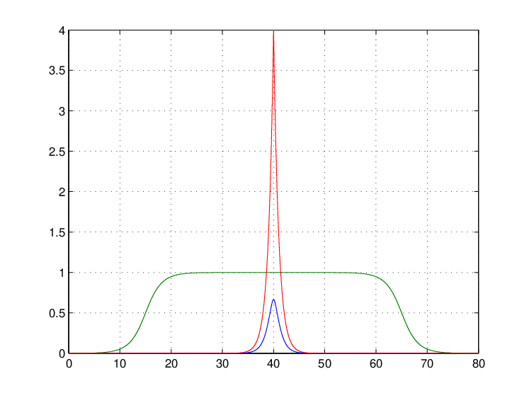
Refer to caption
(a) (∫0x|φ⁡(x−10)−φ⁡(x−10−10−9)|2)1/2≈10−9\left(\int_{0}^{x}|\varphi(x-10)-\varphi(x-10-10^{-9})|^{2}\right)^{1/2}\approx 10^{-9}
Refer to caption
(b) log⁡(∫0x|φ⁡(x−10)−φ⁡(x−10−10−9)|2)1/2≈−20.72\log\left(\int_{0}^{x}|\varphi(x-10)-\varphi(x-10-10^{-9})|^{2}\right)^{1/2}\approx-20.72
Figure 2: Distance between two very close peakons (at time t=10t=10 with respective speeds 11 and OPEN1+10−10)1+10^{-10}).

To prove that the speed of x~i​(⋅)\tilde{x}_{i}(\cdot) stays close to cic_{i}, we set

Sj(t)=φcj(⋅−x~j(t)),ε1(t)=u(t)−∑j=1NSj(t)S_{j}(t)=\varphi_{c_{j}}(\cdot-\tilde{x}_{j}(t)),~~\varepsilon_{1}(t)=u(t)-\sum_{j=1}^{N}S_{j}(t)

and

Rj(t)=ρcj(⋅−x~j(t)),ε2(t)=v(t)−∑j=1NRj(t).R_{j}(t)=\rho_{c_{j}}(\cdot-\tilde{x}_{j}(t)),~~\varepsilon_{2}(t)=v(t)-\sum_{j=1}^{N}R_{j}(t).

One can notice that

∂x2Ri=4​Ri−Si,\partial^{2}_{x}R_{i}=4R_{i}-S_{i}, (4.15)

and using the Fourier transformation

(1−∂x2)−1(4−∂x2)−1(⋅)\displaystyle(1-\partial^{2}_{x})^{-1}(4-\partial^{2}_{x})^{-1}(\cdot) =ℱ−1​[1(1+ω2)​(4+ω2)]​(⋅)\displaystyle=\mathcal{F}^{-1}\left[\frac{1}{(1+\omega^{2})(4+\omega^{2})}\right](\cdot)
=ℱ−1​[13​(1+ω2)−13​(4+ω2)]​(⋅)\displaystyle=\mathcal{F}^{-1}\left[\frac{1}{3(1+\omega^{2})}-\frac{1}{3(4+\omega^{2})}\right](\cdot)
=13(1−∂x2)−1(⋅)−13(4−∂x2)−1(⋅).\displaystyle=\frac{1}{3}(1-\partial^{2}_{x})^{-1}(\cdot)-\frac{1}{3}(4-\partial^{2}_{x})^{-1}(\cdot). (4.16)

Differentiating (4.14) with respect to time and using (4.15), we get

∫ℝ∂tε2​∂xRi=x~˙i​(t)​(4​∫ℝε2​Ri−∫ℝε2​Si)\int_{\mathbb{R}}\partial_{t}\varepsilon_{2}\partial_{x}R_{i}=\dot{\tilde{x}}_{i}(t)\left(4\int_{\mathbb{R}}\varepsilon_{2}R_{i}-\int_{\mathbb{R}}\varepsilon_{2}S_{i}\right)

and thus

|∫ℝ∂tε2​∂xRi|\displaystyle\left|\int_{\mathbb{R}}\partial_{t}\varepsilon_{2}\partial_{x}R_{i}\right| ≤|x~˙i​(t)|​(4​‖ε2‖L∞​(ℝ)​‖Ri‖L1​(ℝ)+‖ε2‖L∞​(ℝ)​‖Si‖L1​(ℝ))\displaystyle\leq|\dot{\tilde{x}}_{i}(t)|\left(4\|\varepsilon_{2}\|_{L^{\infty}(\mathbb{R})}\|R_{i}\|_{L^{1}(\mathbb{R})}+\|\varepsilon_{2}\|_{L^{\infty}(\mathbb{R})}\|S_{i}\|_{L^{1}(\mathbb{R})}\right)
≤|x~˙i​(t)−ci|​O​(γ)+O⁡(γ),\displaystyle\leq|\dot{\tilde{x}}_{i}(t)-c_{i}|O(\gamma)+O(\gamma), (4.17)

we point out that ‖Si‖L1​(ℝ)=c\left\|S_{i}\right\|_{L^{1}(\mathbb{R})}=c and ‖Ri‖L1​(ℝ)=c/2\left\|R_{i}\right\|_{L^{1}(\mathbb{R})}=c/2. Substituting uu by ε1+∑j=1NSj\varepsilon_{1}+\sum_{j=1}^{N}S_{j} in (1.7) and using that SjS_{j} satisfies

∂tSj=−(x~˙j(t)−cj)∂xSj−12∂xSj2−32(1−∂x2)−1∂xSj2,\partial_{t}S_{j}=-(\dot{\tilde{x}}_{j}(t)-c_{j})\partial_{x}S_{j}-\frac{1}{2}\partial_{x}S_{j}^{2}-\frac{3}{2}(1-\partial^{2}_{x})^{-1}\partial_{x}S^{2}_{j},

we infer that ε1\varepsilon_{1} satisfies on [0,t0][0,t_{0}],

∂tε1\displaystyle\partial_{t}\varepsilon_{1} −∑j=1N(x~˙j(t)−cj)∂xSj\displaystyle-\sum_{j=1}^{N}(\dot{\tilde{x}}_{j}(t)-c_{j})\partial_{x}S_{j}
=−12∂x[(ε1+∑j=1NSj)2−∑j=1NSj2]\displaystyle=-\frac{1}{2}\partial_{x}\left[\left(\varepsilon_{1}+\sum_{j=1}^{N}S_{j}\right)^{2}-\sum_{j=1}^{N}S^{2}_{j}\right]
−32∂x(1−∂x2)−1[(ε1+∑j=1NSj)2−∑j=1NSj2].\displaystyle\hskip 28.45274pt-\frac{3}{2}\partial_{x}(1-\partial^{2}_{x})^{-1}\left[\left(\varepsilon_{1}+\sum_{j=1}^{N}S_{j}\right)^{2}-\sum_{j=1}^{N}S^{2}_{j}\right].

Multiplying by (4−∂x2)−1(⋅)(4-\partial^{2}_{x})^{-1}(\cdot) and using (4.16), we get

∂tε2−∑j=1N(x~˙j(t)−cj)∂xRj=−12∂x(1−∂x2)−1[(ε1+∑j=1NSj)2−∑j=1NSj2].\partial_{t}\varepsilon_{2}-\sum_{j=1}^{N}(\dot{\tilde{x}}_{j}(t)-c_{j})\partial_{x}R_{j}=-\frac{1}{2}\partial_{x}(1-\partial^{2}_{x})^{-1}\left[\left(\varepsilon_{1}+\sum_{j=1}^{N}S_{j}\right)^{2}-\sum_{j=1}^{N}S^{2}_{j}\right].

Taking the L2L^{2} scalar product with ∂xRi\partial_{x}R_{i}, integrating by parts, we find

−(x~˙i​(t)CLOSE\displaystyle-(\dot{\tilde{x}}_{i}(t) OPEN−ci)​∫ℝ(∂xRi)2\displaystyle-c_{i})\int_{\mathbb{R}}(\partial_{x}R_{i})^{2}
=−∫ℝ∂tε2∂xRi+∑1≤j≤Nj≠i(x~˙j(t)−cj)∫ℝ(∂xRi)(∂xRj)\displaystyle=-\int_{\mathbb{R}}\partial_{t}\varepsilon_{2}\partial_{x}R_{i}+\sum\limits_{\underset{j\neq i}{1\leq j\leq N}}(\dot{\tilde{x}}_{j}(t)-c_{j})\int_{\mathbb{R}}(\partial_{x}R_{i})(\partial_{x}R_{j})
+12∫ℝ(1−∂x2)−1[(ε1+∑j=1NSj)2−∑j=1NSj2]∂x2Ri.\displaystyle\hskip 28.45274pt+\frac{1}{2}\int_{\mathbb{R}}(1-\partial^{2}_{x})^{-1}\left[\left(\varepsilon_{1}+\sum_{j=1}^{N}S_{j}\right)^{2}-\sum_{j=1}^{N}S^{2}_{j}\right]\partial^{2}_{x}R_{i}. (4.18)

We set

Q=(ε1+∑j=1NSj)2−∑j=1NSj2=ε12+2​ε1​(∑j=1NSj)+∑1≤i,j≤Nj≠iSi​Sj,Q=\left(\varepsilon_{1}+\sum_{j=1}^{N}S_{j}\right)^{2}-\sum_{j=1}^{N}S^{2}_{j}\\ =\varepsilon_{1}^{2}+2\varepsilon_{1}\left(\sum_{j=1}^{N}S_{j}\right)+\sum\limits_{\underset{j\neq i}{1\leq i,j\leq N}}S_{i}S_{j},

then

(1−∂x2)−1Q\displaystyle(1-\partial^{2}_{x})^{-1}Q =(1−∂x2)−1ε12+2∑j=1N(1−∂x2)−1(ε1Sj)+∑1≤i,j≤Nj≠i(1−∂x2)−1(SiSj)\displaystyle=(1-\partial^{2}_{x})^{-1}\varepsilon_{1}^{2}+2\sum_{j=1}^{N}(1-\partial^{2}_{x})^{-1}\left(\varepsilon_{1}S_{j}\right)+\sum\limits_{\underset{j\neq i}{1\leq i,j\leq N}}(1-\partial^{2}_{x})^{-1}\left(S_{i}S_{j}\right)
=I+J+K.\displaystyle=I+J+K.

We have the following estimates

I=12∫ℝe−|x−x′|ε12(x′)≤12∥e−|⋅|∥L∞​(ℝ)∥ε1∥L2​(ℝ)2=12∥ε1∥L2​(ℝ)2,I=\frac{1}{2}\int_{\mathbb{R}}e^{-|x-x^{\prime}|}\varepsilon^{2}_{1}(x^{\prime})\leq\frac{1}{2}\|e^{-|\cdot|}\|_{L^{\infty}(\mathbb{R})}\|\varepsilon_{1}\|^{2}_{L^{2}(\mathbb{R})}=\frac{1}{2}\|\varepsilon_{1}\|^{2}_{L^{2}(\mathbb{R})},
J=∑j=1N∫ℝe−|x−x′|ε1(x′)Sj(x′)≤∥e−|⋅|∥L∞​(ℝ)∥ε1∥L2​(ℝ)∑j=1N∥Sj∥L2​(ℝ)=(∑j=1Ncj)∥ε1∥L2​(ℝ)J=\sum_{j=1}^{N}\int_{\mathbb{R}}e^{-|x-x^{\prime}|}\varepsilon_{1}(x^{\prime})S_{j}(x^{\prime})\leq\|e^{-|\cdot|}\|_{L^{\infty}(\mathbb{R})}\|\varepsilon_{1}\|_{L^{2}(\mathbb{R})}\sum_{j=1}^{N}\|S_{j}\|_{L^{2}(\mathbb{R})}=\left(\sum_{j=1}^{N}c_{j}\right)\|\varepsilon_{1}\|_{L^{2}(\mathbb{R})}

and

K=12​∑1≤i,j≤Nj≠i∫ℝe−|x−x′|​Sj​(x′)​Si​(x′)≤12​∑1≤i,j≤Nj≠i∫ℝSj​(x′)​Si​(x′).K=\frac{1}{2}\sum\limits_{\underset{j\neq i}{1\leq i,j\leq N}}\int_{\mathbb{R}}e^{-|x-x^{\prime}|}S_{j}(x^{\prime})S_{i}(x^{\prime})\leq\frac{1}{2}\sum\limits_{\underset{j\neq i}{1\leq i,j\leq N}}\int_{\mathbb{R}}S_{j}(x^{\prime})S_{i}(x^{\prime}).

Thus, using (4.4) and the exponential decay of SjS_{j}, it holds

∥(1−∂x2)−1Q∥L∞​(ℝ)≤O(γ)+O(e−L/4)\|(1-\partial^{2}_{x})^{-1}Q\|_{L^{\infty}(\mathbb{R})}\leq O(\gamma)+O(e^{-L/4})

and then

|12∫ℝ[(1−∂x2)−1Q]∂x2Ri|\displaystyle\left|\frac{1}{2}\int_{\mathbb{R}}[(1-\partial^{2}_{x})^{-1}Q]\partial^{2}_{x}R_{i}\right| ≤12∥(1−∂x2)−1Q∥L∞​(ℝ)∥∂x2Ri∥L1​(ℝ)\displaystyle\leq\frac{1}{2}\|(1-\partial^{2}_{x})^{-1}Q\|_{L^{\infty}(\mathbb{R})}\|\partial^{2}_{x}R_{i}\|_{L^{1}(\mathbb{R})}
≤O(γ)+O(e−L/4),\displaystyle\leq O(\gamma)+O(e^{-L/4}), (4.19)

where ‖∂x2Ri‖L1​(ℝ)=c/3\left\|\partial^{2}_{x}R_{i}\right\|_{L^{1}(\mathbb{R})}=c/3. Now, combining (4.17), (4.19), and using the exponential decay of ∂xRi\partial_{x}R_{i}, it holds

|x~˙i(t)−ci|∥∂xRi∥L2​(ℝ)2≤|x~˙i(t)−ci|O(γ)+O(γ)+O(e−L/4),\left|\dot{\tilde{x}}_{i}(t)-c_{i}\right|\|\partial_{x}R_{i}\|^{2}_{L^{2}(\mathbb{R})}\leq\left|\dot{\tilde{x}}_{i}(t)-c_{i}\right|O(\gamma)+O(\gamma)+O(e^{-L/4}),

then

|x~˙i(t)−ci|(ci254−O(γ))≤O(γ)+O(e−L/4),\left|\dot{\tilde{x}}_{i}(t)-c_{i}\right|\left(\frac{c_{i}^{2}}{54}-O(\gamma)\right)\leq O(\gamma)+O(e^{-L/4}),

which yields (4.6).

Taking 0<γ<γ00<\gamma<\gamma_{0} and L>L0>0L>L_{0}>0 with γ0≪1\gamma_{0}\ll 1 and L0≫1L_{0}\gg 1, combining (1.12)-(1.14), (4.6) and (4.13), we deduce that

x~i​(t)−x~i−1​(t)\displaystyle\tilde{x}_{i}(t)-\tilde{x}_{i-1}(t) =x~i​(0)−x~i−1​(0)+(ci−ci−1)​t\displaystyle=\tilde{x}_{i}(0)-\tilde{x}_{i-1}(0)+(c_{i}-c_{i-1})t
≥L−2​C0​γ0+(ci−ci−1)​t2\displaystyle\geq L-2C_{0}\gamma_{0}+\frac{(c_{i}-c_{i-1})t}{2}
≥3​L4+(ci−ci−1)​t2,\displaystyle\geq\frac{3L}{4}+\frac{(c_{i}-c_{i-1})t}{2},

this proves (4.7).

From (4.5), we infer that

v⁡(x)=∑j=1Nρcj​(x−x~j)+O⁡(γ),∀x∈ℝ,v(x)=\sum_{j=1}^{N}\rho_{c_{j}}(x-\tilde{x}_{j})+O(\gamma),~~\forall x\in\mathbb{R},

please note that we abuse notation by writing ε2​(x)=O​(γ)\varepsilon_{2}(x)=O(\gamma). Applying this formula with x=ξ1ix=\xi^{i}_{1} and v⁡(ξ1i)=maxx∈Ji⁡v⁡(x)v(\xi^{i}_{1})=\max_{x\in J_{i}}v(x), and using (4.7), it holds

v⁡(ξ1i)\displaystyle v(\xi^{i}_{1}) =maxx∈Ji⁡{∑j=1Nρcj​(x−x~j)}+O⁡(γ)\displaystyle=\max_{x\in J_{i}}\left\{\sum_{j=1}^{N}\rho_{c_{j}}(x-\tilde{x}_{j})\right\}+O(\gamma)
=ci6+O(e−L/4)+O(γ)\displaystyle=\frac{c_{i}}{6}+O(e^{-L/4})+O(\gamma)
≥ci7.\displaystyle\geq\frac{c_{i}}{7}.

On the other hand, for x∈Ji∖[x~i​(t)−L/12,x~i​(t)+L/12]x\in J_{i}\setminus[\tilde{x}_{i}(t)-L/12,~\tilde{x}_{i}(t)+L/12], we get

v(x)≤ci3e−L/12+O(e−L/4)+O(γ)≤ci8.v(x)\leq\frac{c_{i}}{3}e^{-L/12}+O(e^{-L/4})+O(\gamma)\\ \leq\frac{c_{i}}{8}.

This ensures that ξ1i∈[x~i​(t)−L/12,x~i​(t)+L/12]\xi^{i}_{1}\in[\tilde{x}_{i}(t)-L/12,~\tilde{x}_{i}(t)+L/12], and this concluded the proof of the lemma. □\square

4.2 Monotonicity property

Thanks to the preceding lemma, for ε0>0\varepsilon_{0}>0 small enough and L0>0L_{0}>0 large enough, one can construct N​C1N~C^{1} functions x~1,…,x~N\tilde{x}_{1},\ldots,\tilde{x}_{N} defined on [0,t0][0,t_{0}] such that (4.4)-(4.8) are satisfied. In this subsection, we state the almost monotonicity of functionals that are very close to the energy at the right of iith bump, i=1,…,N−1i=1,\ldots,N-1 of uu (respectively of vv). Let ψ\psi be a C∞C^{\infty} test-function (see Fig. 3) such that

{0<ψ⁡(x)​<1,ψ′​(x)>​0,x∈ℝ,|ψ(q)(x)|≤10ψ′(x),q=2,3,4,5,x∈[−10,10],\left\{\begin{aligned} &0<\psi(x)<1,~\psi^{\prime}(x)>0,&x&\in\mathbb{R},\\ &|\psi^{(q)}(x)|\leq 10\psi^{\prime}(x),~q=2,3,4,5,&x&\in[-10,10],\\ \end{aligned}\right. (4.20)

and

ψ(x)={e−|x|,x<−10,1−e−|x|,x>10.\psi(x)=\left\{\begin{aligned} &e^{-|x|},&x&<-10,\\ &1-e^{-|x|},&x&>10.\\ \end{aligned}\right. (4.21)
Refer to caption
Figure 3: ψ(q)​(x)\psi^{(q)}(x), q=0,1,2,3,4,5q=0,1,2,3,4,5, profiles. Note that ψ(5)\psi^{(5)} will not be used.

Setting ψK=ψ(⋅/K)\psi_{K}=\psi(\cdot/K), we introduce for i=2,…,Ni=2,\ldots,N,

𝒥i,K​(t)=∫ℝ(4​v2+5​vx2+vx​x2)​ψi,K​(t),\mathcal{J}_{i,K}(t)=\int_{\mathbb{R}}\left(4v^{2}+5v^{2}_{x}+v^{2}_{xx}\right)\psi_{i,K}(t), (4.22)

where ψi,K​(t,x)=ψK​(x−yi​(t))\psi_{i,K}(t,x)=\psi_{K}(x-y_{i}(t)) with yiy_{i}’s as in (4.8). Note that 𝒥i,K​(t)\mathcal{J}_{i,K}(t) is close to ‖u⁡(t)‖ℋ​(x>yi​(t))2\|u(t)\|^{2}_{\mathcal{H}(x>y_{i}(t))} (respectively to ‖v⁡(t)‖H2​(x>yi​(t))2\|v(t)\|^{2}_{H^{2}(x>y_{i}(t))}) and thus measures the energy at the right of the (i−1)(i-1)th bump of uu (respectively of vv). Finally, we set

σ0=14​min⁡{c1,c2−c1,…,cN−cN−1}.\sigma_{0}=\frac{1}{4}\min\{c_{1},c_{2}-c_{1},\ldots,c_{N}-c_{N-1}\}. (4.23)

We have the following monotonicity result.

Proposition 4.1 (Exponential Decay of the Functional 𝒥i,K​(t)\mathcal{J}_{i,K}(t)).

Let u∈𝒳([0,T[)u\in\mathcal{X}([0,T[), with 0<T≤+∞0<T\leq+\infty, be a solution of equation (1.1) that satisfies (1.12)-(1.14) and (4.4)-(4.5). There exist γ0>0\gamma_{0}>0 and L0>0L_{0}>0 only depending on c1c_{1} such that if 0<γ<γ00<\gamma<\gamma_{0} and L>L0>0L>L_{0}>0, then for any 4≤K≲L4\leq K\lesssim\sqrt{L},

𝒥i,K(t)−𝒥i,K(0)≤O(e−L8​K),∀t∈[0,t0],i=2,…,N.\mathcal{J}_{i,K}(t)-\mathcal{J}_{i,K}(0)\leq O(e^{-\frac{L}{8K}}),~~\forall t\in[0,t_{0}],~~i=2,\ldots,N. (4.24)

The proof of Proposition 4.1 relies on the following Virial type identity.

Lemma 4.2 (Virial Type Identity).

Let u∈𝒳([0,T[)u\in\mathcal{X}([0,T[), with 0<T≤+∞0<T\leq+\infty, be a solution of equation (1.1) that satisfies (1.12)-(1.14). For any smooth space function g:ℝ↦ℝg:\mathbb{R}\mapsto\mathbb{R}, it holds

dd​t∫ℝ\displaystyle\frac{d}{dt}\int_{\mathbb{R}} (4​v2+5​vx2+vx​x2)​g\displaystyle\left(4v^{2}+5v^{2}_{x}+v^{2}_{xx}\right)g
=23​∫ℝu3​g′−4​∫ℝu2​v​g′−12​∫ℝu2​v​g′′′+12​∫ℝu2​vx​g′′+∫ℝu​h​g′\displaystyle=\frac{2}{3}\int_{\mathbb{R}}u^{3}g^{\prime}-4\int_{\mathbb{R}}u^{2}vg^{\prime}-\frac{1}{2}\int_{\mathbb{R}}u^{2}vg^{\prime\prime\prime}+\frac{1}{2}\int_{\mathbb{R}}u^{2}v_{x}g^{\prime\prime}+\int_{\mathbb{R}}uhg^{\prime}
+12∫ℝuhxg′′−52∫ℝvhxg′′−2∫ℝvxhg′′+12∫ℝvhxg(4)\displaystyle\hskip 28.45274pt+\frac{1}{2}\int_{\mathbb{R}}uh_{x}g^{\prime\prime}-\frac{5}{2}\int_{\mathbb{R}}vh_{x}g^{\prime\prime}-2\int_{\mathbb{R}}v_{x}hg^{\prime\prime}+\frac{1}{2}\int_{\mathbb{R}}vh_{x}g^{(4)} (4.25)

where y=(1−∂x2)uy=(1-\partial^{2}_{x})u, v=(4−∂x2)−1uv=(4-\partial^{2}_{x})^{-1}u and h=(1−∂x2)−1u2h=(1-\partial^{2}_{x})^{-1}u^{2}.

The full proof of Lemma 4.2 is given in the Appendix 4.

Proof of Proposition 4.1. We first note that, combining (4.6) and (4.8), it holds for i=2,…,Ni=2,\ldots,N,

y˙i​(t)\displaystyle\dot{y}_{i}(t) =x~˙i−1​(t)+x~˙i​(t)2\displaystyle=\frac{\dot{\tilde{x}}_{i-1}(t)+\dot{\tilde{x}}_{i}(t)}{2}
=ci−1+ci2+O⁡(γ)\displaystyle=\frac{c_{i-1}+c_{i}}{2}+O(\gamma)
≥ci−1+O⁡(γ)\displaystyle\geq c_{i-1}+O(\gamma)
≥c12.\displaystyle\geq\frac{c_{1}}{2}. (4.26)

Recall that the assumption (1.12) ensures that u≥0u\geq 0 and v≥0v\geq 0 on ℝ\mathbb{R}. Now, applying the Virial type identity (4.25) with g=ψi,Kg=\psi_{i,K} and using (4.26), we get

dd​t​𝒥i,K​(t)\displaystyle\frac{d}{dt}\mathcal{J}_{i,K}(t) =−y˙i∫ℝ(4v2+5vx2+vx​x2)ψi,K′+23∫ℝu3ψi,K′−4∫ℝu2vψi,K′\displaystyle=-\dot{y}_{i}\int_{\mathbb{R}}\left(4v^{2}+5v^{2}_{x}+v^{2}_{xx}\right)\psi^{\prime}_{i,K}+\frac{2}{3}\int_{\mathbb{R}}u^{3}\psi_{i,K}^{\prime}-4\int_{\mathbb{R}}u^{2}v\psi_{i,K}^{\prime}
−12∫ℝu2vψi,K′′′+12∫ℝu2vxψ′′i,K+∫ℝuhψi,K′+12∫ℝuhxψi,K′′\displaystyle\hskip 28.45274pt-\frac{1}{2}\int_{\mathbb{R}}u^{2}v\psi_{i,K}^{\prime\prime\prime}+\frac{1}{2}\int_{\mathbb{R}}u^{2}v_{x}\psi^{\prime\prime}_{i,K}+\int_{\mathbb{R}}uh\psi_{i,K}^{\prime}+\frac{1}{2}\int_{\mathbb{R}}uh_{x}\psi_{i,K}^{\prime\prime}
−52∫ℝvhxψ′′i,K−2∫ℝvxhψ′′i,K+12∫ℝvhxψ(4)i,K\displaystyle\hskip 56.9055pt-\frac{5}{2}\int_{\mathbb{R}}vh_{x}\psi^{\prime\prime}_{i,K}-2\int_{\mathbb{R}}v_{x}h\psi^{\prime\prime}_{i,K}+\frac{1}{2}\int_{\mathbb{R}}vh_{x}\psi^{(4)}_{i,K}
≤−y˙i∫ℝ(4v2+5vx2+vx​x2)ψi,K′+23∫ℝu3ψi,K′−12∫ℝu2vψi,K′′′\displaystyle\leq-\dot{y}_{i}\int_{\mathbb{R}}\left(4v^{2}+5v^{2}_{x}+v^{2}_{xx}\right)\psi^{\prime}_{i,K}+\frac{2}{3}\int_{\mathbb{R}}u^{3}\psi_{i,K}^{\prime}-\frac{1}{2}\int_{\mathbb{R}}u^{2}v\psi^{\prime\prime\prime}_{i,K}
+12∫ℝu2vxψi,K′′+∫ℝuhψi,K′+12∫ℝuhxψi,K′′−52∫ℝvhxψ′′i,K\displaystyle\hskip 28.45274pt+\frac{1}{2}\int_{\mathbb{R}}u^{2}v_{x}\psi_{i,K}^{\prime\prime}+\int_{\mathbb{R}}uh\psi_{i,K}^{\prime}+\frac{1}{2}\int_{\mathbb{R}}uh_{x}\psi_{i,K}^{\prime\prime}-\frac{5}{2}\int_{\mathbb{R}}vh_{x}\psi^{\prime\prime}_{i,K}
−2∫ℝvxhψ′′i,K+12∫ℝvhxψ(4)i,K\displaystyle\hskip 56.9055pt-2\int_{\mathbb{R}}v_{x}h\psi^{\prime\prime}_{i,K}+\frac{1}{2}\int_{\mathbb{R}}vh_{x}\psi^{(4)}_{i,K}
≤−c12∫ℝ(4v2+5vx2+vx​x2)ψi,K′+∑k=18Jk.\displaystyle\leq-\frac{c_{1}}{2}\int_{\mathbb{R}}\left(4v^{2}+5v^{2}_{x}+v^{2}_{xx}\right)\psi^{\prime}_{i,K}+\sum_{k=1}^{8}J_{k}. (4.27)

We claim that for k=1,…,8k=1,\ldots,8, it holds

Jk≤c120​∫ℝ(4​v2+5​vx2+vx​x2)​ψi,K′+CK​‖u0‖ℋ3​e−1K​(σ0​t+L/8).J_{k}\leq\frac{c_{1}}{20}\int_{\mathbb{R}}\left(4v^{2}+5v^{2}_{x}+v^{2}_{xx}\right)\psi^{\prime}_{i,K}+\frac{C}{K}\|u_{0}\|^{3}_{\mathcal{H}}e^{-\frac{1}{K}(\sigma_{0}t+L/8)}. (4.28)

We divide ℝ\mathbb{R} into two regions DiD_{i} and DicD^{c}_{i} with

Di=[x~i−1(t)+L4,x~i(t)−L4],i=2,…,N.D_{i}=\left[\tilde{x}_{i-1}(t)+\frac{L}{4},\tilde{x}_{i}(t)-\frac{L}{4}\right],~~i=2,\ldots,N.

Combining (4.7) and (4.8), one can check that for x∈Dicx\in D^{c}_{i},

|x−yi​(t)|\displaystyle|x-y_{i}(t)| ≥x~i​(t)−x~i−1​(t)2−L4\displaystyle\geq\frac{\tilde{x}_{i}(t)-\tilde{x}_{i-1}(t)}{2}-\frac{L}{4}
≥ci−ci−14​t+L8\displaystyle\geq\frac{c_{i}-c_{i-1}}{4}t+\frac{L}{8}
≥σ0​t+L8.\displaystyle\geq\sigma_{0}t+\frac{L}{8}. (4.29)

Let us begin by an estimate of J1J_{1}. Using (2.3), (4.29) and the exponential decay of ψi,K′\psi^{\prime}_{i,K} on DicD^{c}_{i}, we get

23​∫ℝu3​ψi,K′\displaystyle\frac{2}{3}\int_{\mathbb{R}}u^{3}\psi^{\prime}_{i,K} =23​∫Diu3​ψi,K′+23​∫Dicu3​ψi,K′\displaystyle=\frac{2}{3}\int_{D_{i}}u^{3}\psi_{i,K}^{\prime}+\frac{2}{3}\int_{D^{c}_{i}}u^{3}\psi^{\prime}_{i,K}
≤23​‖u‖L∞​(Di)​∫ℝu2​ψi,K′+23​‖ψi,K′‖L∞​(Dic)​‖u‖L∞​(ℝ)​‖u‖L2​(ℝ)2\displaystyle\leq\frac{2}{3}\|u\|_{L^{\infty}(D_{i})}\int_{\mathbb{R}}u^{2}\psi^{\prime}_{i,K}+\frac{2}{3}\|\psi^{\prime}_{i,K}\|_{L^{\infty}(D^{c}_{i})}\|u\|_{L^{\infty}(\mathbb{R})}\|u\|^{2}_{L^{2}(\mathbb{R})}
≤23​‖u‖L∞​(Di)​∫ℝu2​ψi,K′+CK​‖u‖L2​(ℝ)3​e−1K​(σ0​t+L/8).\displaystyle\leq\frac{2}{3}\|u\|_{L^{\infty}(D_{i})}\int_{\mathbb{R}}u^{2}\psi^{\prime}_{i,K}+\frac{C}{K}\|u\|^{3}_{L^{2}(\mathbb{R})}e^{-\frac{1}{K}(\sigma_{0}t+L/8)}. (4.30)

Note that, using the exponential decay of |ψj,K′′′||\psi^{\prime\prime\prime}_{j,K}| on DicD^{c}_{i}, |ψi,K′′′|≤(10/K2)​ψi,K′|\psi^{\prime\prime\prime}_{i,K}|\leq(10/K^{2})\psi^{\prime}_{i,K} on DiD_{i}, with K≥4K\geq 4, and that ‖u‖ℋ=‖u0‖ℋ\|u\|_{\mathcal{H}}=\|u_{0}\|_{\mathcal{H}}, we have

∫ℝu2​ψi,K′\displaystyle\int_{\mathbb{R}}u^{2}\psi^{\prime}_{i,K} =∫ℝ(4​v−vx​x)2​ψi,K′\displaystyle=\int_{\mathbb{R}}(4v-v_{xx})^{2}\psi^{\prime}_{i,K}
=16​∫ℝv2​ψi,K′+∫ℝvx​x2​ψi,K′−8​∫ℝv​vx​x​ψi,K′\displaystyle=16\int_{\mathbb{R}}v^{2}\psi^{\prime}_{i,K}+\int_{\mathbb{R}}v^{2}_{xx}\psi^{\prime}_{i,K}-8\int_{\mathbb{R}}vv_{xx}\psi^{\prime}_{i,K}
=16​∫ℝv2​ψi,K′+∫ℝvx​x2​ψi,K′+8​∫ℝvx2​ψi,K′+4​∫ℝ∂x(v2)​ψi,K′′\displaystyle=16\int_{\mathbb{R}}v^{2}\psi^{\prime}_{i,K}+\int_{\mathbb{R}}v^{2}_{xx}\psi^{\prime}_{i,K}+8\int_{\mathbb{R}}v^{2}_{x}\psi^{\prime}_{i,K}+4\int_{\mathbb{R}}\partial_{x}(v^{2})\psi^{\prime\prime}_{i,K}
=16​∫ℝv2​ψi,K′+∫ℝvx​x2​ψi,K′+8​∫ℝvx2​ψi,K′−4​∫ℝv2​ψi,K′′′\displaystyle=16\int_{\mathbb{R}}v^{2}\psi^{\prime}_{i,K}+\int_{\mathbb{R}}v^{2}_{xx}\psi^{\prime}_{i,K}+8\int_{\mathbb{R}}v^{2}_{x}\psi^{\prime}_{i,K}-4\int_{\mathbb{R}}v^{2}\psi^{\prime\prime\prime}_{i,K}
≤∫ℝ(16​v2+8​vx2+vx​x2)​ψi,K′+4​∫Div2​|ψj,K′′′|+4​∫Dicv2​|ψj,K′′′|\displaystyle\leq\int_{\mathbb{R}}\left(16v^{2}+8v^{2}_{x}+v^{2}_{xx}\right)\psi^{\prime}_{i,K}+4\int_{D_{i}}v^{2}|\psi^{\prime\prime\prime}_{j,K}|+4\int_{D^{c}_{i}}v^{2}|\psi^{\prime\prime\prime}_{j,K}|
≤∫ℝ(16​v2+8​vx2+vx​x2)​ψi,K′+40K2​∫ℝv2​ψi,K′+CK3​‖u0‖ℋ2​e−1K​(σ0​t+L/8)\displaystyle\leq\int_{\mathbb{R}}\left(16v^{2}+8v^{2}_{x}+v^{2}_{xx}\right)\psi^{\prime}_{i,K}+\frac{40}{K^{2}}\int_{\mathbb{R}}v^{2}\psi^{\prime}_{i,K}+\frac{C}{K^{3}}\|u_{0}\|^{2}_{\mathcal{H}}e^{-\frac{1}{K}(\sigma_{0}t+L/8)}
≤5​∫ℝ(4​v2+5​vx2+vx​x2)​ψi,K′+CK3​‖u0‖ℋ2​e−1K​(σ0​t+L/8).\displaystyle\leq 5\int_{\mathbb{R}}\left(4v^{2}+5v^{2}_{x}+v^{2}_{xx}\right)\psi^{\prime}_{i,K}+\frac{C}{K^{3}}\|u_{0}\|^{2}_{\mathcal{H}}e^{-\frac{1}{K}(\sigma_{0}t+L/8)}. (4.31)

Now, using the exponential decay of φci\varphi_{c_{i}} on DiD_{i}, (4.4), and proceeding as for the estimate (3.10) (see Lemma 3.2), it holds

‖u‖L∞​(Di)\displaystyle\|u\|_{L^{\infty}(D_{i})} ≤‖u−∑j=1Nφcj(⋅−x~j(t))‖L∞​(Di)+∑j=1N‖φcj(⋅−x~j(t))‖L∞​(Di)\displaystyle\leq\left\|u-\sum_{j=1}^{N}\varphi_{c_{j}}(\cdot-\tilde{x}_{j}(t))\right\|_{L^{\infty}(D_{i})}+\sum_{j=1}^{N}\left\|\varphi_{c_{j}}(\cdot-\tilde{x}_{j}(t))\right\|_{L^{\infty}(D_{i})}
≤O(γ1/2)+O(e−L/8).\displaystyle\leq O(\gamma^{1/2})+O(e^{-L/8}). (4.32)

Therefore, for 0<γ<γ00<\gamma<\gamma_{0} and L>L0>0L>L_{0}>0, with γ0≪1\gamma_{0}\ll 1 and L0≫1L_{0}\gg 1, combining (4.30)-(4.31), we obtain

J1≤c120​∫ℝ(4​v2+5​vx2+vx​x2)​ψi,K′+CK​‖u‖L2​(ℝ)3​e−1K​(σ0​t+L/8).J_{1}\leq\frac{c_{1}}{20}\int_{\mathbb{R}}\left(4v^{2}+5v^{2}_{x}+v^{2}_{xx}\right)\psi^{\prime}_{i,K}+\frac{C}{K}\|u\|^{3}_{L^{2}(\mathbb{R})}e^{-\frac{1}{K}(\sigma_{0}t+L/8)}.

Next, the estimate of J2J_{2} on DicD^{c}_{i} gives us

|12​∫Dicu2​v​ψi,K′′′|≤12​‖ψi,K′′′‖L∞​(Dic)​‖v‖L∞​(ℝ)​‖u‖L2​(ℝ)2.\left|\frac{1}{2}\int_{D^{c}_{i}}u^{2}v\psi^{\prime\prime\prime}_{i,K}\right|\leq\frac{1}{2}\|\psi^{\prime\prime\prime}_{i,K}\|_{L^{\infty}(D^{c}_{i})}\|v\|_{L^{\infty}(\mathbb{R})}\|u\|^{2}_{L^{2}(\mathbb{R})}.

Note that, applying the Hölder inequality, we have for all x∈ℝx\in\mathbb{R},

v⁡(x)\displaystyle v(x) =14​∫ℝe−2​|x−x′|​u​(x′)​d​x′\displaystyle=\frac{1}{4}\int_{\mathbb{R}}e^{-2|x-x^{\prime}|}u(x^{\prime})dx^{\prime}
≤14​(∫ℝe−4​|x−x′|​d​x′)1/2​(∫ℝ|u⁡(x′)|2​d​x′)1/2\displaystyle\leq\frac{1}{4}\left(\int_{\mathbb{R}}e^{-4|x-x^{\prime}|}dx^{\prime}\right)^{1/2}\left(\int_{\mathbb{R}}|u(x^{\prime})|^{2}dx^{\prime}\right)^{1/2}
=14​2​‖u‖L2​(ℝ)\displaystyle=\frac{1}{4\sqrt{2}}\|u\|_{L^{2}(\mathbb{R})} (4.33)

and thus, using (4.33) and the exponential decay of |ψi,K′′′||\psi^{\prime\prime\prime}_{i,K}| on DicD^{c}_{i}, it holds

|12​∫Dicu2​v​ψi,K′′′|≤18​2​K3​‖u‖L2​(ℝ)3​e−1K​(σ0​t+L/8).\left|\frac{1}{2}\int_{D^{c}_{i}}u^{2}v\psi^{\prime\prime\prime}_{i,K}\right|\leq\frac{1}{8\sqrt{2}K^{3}}\|u\|^{3}_{L^{2}(\mathbb{R})}e^{-\frac{1}{K}(\sigma_{0}t+L/8)}. (4.34)

Using that |ψi,K′′′|≤(10/K2)​ψi,K′|\psi^{\prime\prime\prime}_{i,K}|\leq(10/K^{2})\psi^{\prime}_{i,K} on DiD_{i}, the estimate of J2J_{2} on DiD_{i} leads to

|12​∫Diu2​v​ψi,K′′′|≤5K2​‖u‖L∞​(Di)​∫ℝu​v​ψi,K′.\left|\frac{1}{2}\int_{D_{i}}u^{2}v\psi^{\prime\prime\prime}_{i,K}\right|\leq\frac{5}{K^{2}}\|u\|_{L^{\infty}(D_{i})}\int_{\mathbb{R}}uv\psi^{\prime}_{i,K}. (4.35)

Also, one can notice that, using the exponential decay of |ψj,K′′′||\psi^{\prime\prime\prime}_{j,K}| on DicD^{c}_{i}, |ψi,K′′′|≤(10/K2)​ψi,K′|\psi^{\prime\prime\prime}_{i,K}|\leq(10/K^{2})\psi^{\prime}_{i,K} on ℝ\mathbb{R}, with K≥4K\geq 4, and that ‖u‖ℋ=‖u0‖ℋ\|u\|_{\mathcal{H}}=\|u_{0}\|_{\mathcal{H}}, we have

∫ℝu​v​ψi,K′\displaystyle\int_{\mathbb{R}}uv\psi^{\prime}_{i,K} =∫ℝ(4​v−vx​x)​v​ψi,K′\displaystyle=\int_{\mathbb{R}}(4v-v_{xx})v\psi^{\prime}_{i,K}
=4​∫ℝv2​ψi,K′+∫ℝ∂x(v​ψi,K′)​vx\displaystyle=4\int_{\mathbb{R}}v^{2}\psi^{\prime}_{i,K}+\int_{\mathbb{R}}\partial_{x}(v\psi^{\prime}_{i,K})v_{x}
=4​∫ℝv2​ψj,K′+∫ℝvx2​ψi,K′+∫ℝv​vx​ψi,K′′\displaystyle=4\int_{\mathbb{R}}v^{2}\psi^{\prime}_{j,K}+\int_{\mathbb{R}}v^{2}_{x}\psi^{\prime}_{i,K}+\int_{\mathbb{R}}vv_{x}\psi^{\prime\prime}_{i,K}
=∫ℝ(4​v2+vx2)​ψi,K′−12​∫ℝv2​ψi,K′′′\displaystyle=\int_{\mathbb{R}}\left(4v^{2}+v^{2}_{x}\right)\psi^{\prime}_{i,K}-\frac{1}{2}\int_{\mathbb{R}}v^{2}\psi^{\prime\prime\prime}_{i,K}
≤∫ℝ(4​v2+vx2)​ψi,K′+12​∫Div2​|ψi,K′′′|+12​∫Dicv2​|ψi,K′′′|\displaystyle\leq\int_{\mathbb{R}}\left(4v^{2}+v^{2}_{x}\right)\psi^{\prime}_{i,K}+\frac{1}{2}\int_{D_{i}}v^{2}|\psi^{\prime\prime\prime}_{i,K}|+\frac{1}{2}\int_{D^{c}_{i}}v^{2}|\psi^{\prime\prime\prime}_{i,K}|
≤∫ℝ(4​v2+vx2)​ψi,K′+5K2​∫ℝv2​ψi,K′+CK3​‖u0‖ℋ2​e−1K​(σ0​t+L/8)\displaystyle\leq\int_{\mathbb{R}}\left(4v^{2}+v^{2}_{x}\right)\psi^{\prime}_{i,K}+\frac{5}{K^{2}}\int_{\mathbb{R}}v^{2}\psi^{\prime}_{i,K}+\frac{C}{K^{3}}\|u_{0}\|^{2}_{\mathcal{H}}e^{-\frac{1}{K}(\sigma_{0}t+L/8)}
≤2​∫ℝ(4​v2+5​vx2+vx​x2)​ψi,K′+CK3​‖u0‖ℋ2​e−1K​(σ0​t+L/8).\displaystyle\leq 2\int_{\mathbb{R}}\left(4v^{2}+5v^{2}_{x}+v^{2}_{xx}\right)\psi^{\prime}_{i,K}+\frac{C}{K^{3}}\|u_{0}\|^{2}_{\mathcal{H}}e^{-\frac{1}{K}(\sigma_{0}t+L/8)}. (4.36)

Therefore, for 0<γ<γ00<\gamma<\gamma_{0} and L>L0>0L>L_{0}>0, with γ0≪1\gamma_{0}\ll 1 and L0≫1L_{0}\gg 1, combining (4.32), (4.34)-(4.36), it holds

J2≤c120​∫ℝ(4​v2+5​vx2+vx​x2)​ψi,K′+CK3​‖u‖L2​(ℝ)3​e−1K​(σ0​t+L/8).J_{2}\leq\frac{c_{1}}{20}\int_{\mathbb{R}}\left(4v^{2}+5v^{2}_{x}+v^{2}_{xx}\right)\psi^{\prime}_{i,K}+\frac{C}{K^{3}}\|u\|^{3}_{L^{2}(\mathbb{R})}e^{-\frac{1}{K}(\sigma_{0}t+L/8)}.

In the same way, using that |vx|≤2​v|v_{x}|\leq 2v on ℝ\mathbb{R} (see (3.39)), and the definition of ψi,K\psi_{i,K} (see (4.20) and (4.21)), we deduce the estimate of J3J_{3}.

Let us tackle now the estimate of J4J_{4}. On DicD^{c}_{i} we have

∫Dicu​h​ψi,K′\displaystyle\int_{D^{c}_{i}}uh\psi_{i,K}^{\prime} ≤|ψi,K′|∫ℝL∞​(Dic)⁡u​h\displaystyle\leq\|\psi^{\prime}_{i,K}\|_{L^{\infty}(D^{c}_{i})}\int_{\mathbb{R}}uh
=∥ψi,K′∥L∞​(Dic)∫ℝu[(1−∂x2)−1u2]\displaystyle=\|\psi^{\prime}_{i,K}\|_{L^{\infty}(D^{c}_{i})}\int_{\mathbb{R}}u[(1-\partial^{2}_{x})^{-1}u^{2}]
=∥ψi,K′∥L∞​(Dic)∫ℝu2[(1−∂x2)−1u]\displaystyle=\|\psi^{\prime}_{i,K}\|_{L^{\infty}(D^{c}_{i})}\int_{\mathbb{R}}u^{2}[(1-\partial^{2}_{x})^{-1}u]
≤∥ψi,K′∥L∞​(Djc)∥(1−∂x2)−1u∥L∞​(ℝ)∥u∥L2​(ℝ)2.\displaystyle\leq\|\psi^{\prime}_{i,K}\|_{L^{\infty}(D^{c}_{j})}\|(1-\partial^{2}_{x})^{-1}u\|_{L^{\infty}(\mathbb{R})}\|u\|^{2}_{L^{2}(\mathbb{R})}.

Remark that, applying the Hölder inequality, we have for all x∈ℝx\in\mathbb{R},

(1−∂x2)−1u(x)\displaystyle(1-\partial^{2}_{x})^{-1}u(x) ≤12​∫ℝe−|x−x′|​u​(x′)​d​x′\displaystyle\leq\frac{1}{2}\int_{\mathbb{R}}e^{-|x-x^{\prime}|}u(x^{\prime})dx^{\prime}
≤12​(∫ℝe−2​|x−x′|​d​x′)1/2​(∫ℝ|u⁡(x′)|2​d​x′)1/2\displaystyle\leq\frac{1}{2}\left(\int_{\mathbb{R}}e^{-2|x-x^{\prime}|}dx^{\prime}\right)^{1/2}\left(\int_{\mathbb{R}}|u(x^{\prime})|^{2}dx^{\prime}\right)^{1/2}
=12​‖u‖L2​(ℝ)\displaystyle=\frac{1}{2}\|u\|_{L^{2}(\mathbb{R})} (4.37)

and thus, using (4.37) and the exponential decay of ψi,K′\psi^{\prime}_{i,K} on DicD^{c}_{i}, it holds

∫Dicu​h​ψi,K′≤12​K​‖u‖L2​(ℝ)3​e−1K​(σ0​t+L/8).\int_{D^{c}_{i}}uh\psi^{\prime}_{i,K}\leq\frac{1}{2K}\|u\|^{3}_{L^{2}(\mathbb{R})}e^{-\frac{1}{K}(\sigma_{0}t+L/8)}. (4.38)

The estimate of J4J_{4} on DiD_{i} leads to

∫Diu​h​ψi,K′\displaystyle\int_{D_{i}}uh\psi^{\prime}_{i,K} ≤∥u∥L∞​(Di)∫ℝψi,K′[(1−∂x2)−1u2]\displaystyle\leq\|u\|_{L^{\infty}(D_{i})}\int_{\mathbb{R}}\psi^{\prime}_{i,K}[(1-\partial^{2}_{x})^{-1}u^{2}]
=∥u∥L∞​(Di)∫ℝu2[(1−∂x2)−1ψi,K′].\displaystyle=\|u\|_{L^{\infty}(D_{i})}\int_{\mathbb{R}}u^{2}[(1-\partial^{2}_{x})^{-1}\psi^{\prime}_{i,K}]. (4.39)

On the other hand, using that |ψi,K′′′|≤(10/K2)​ψi,K′|\psi^{\prime\prime\prime}_{i,K}|\leq(10/K^{2})\psi^{\prime}_{i,K} on ℝ\mathbb{R}, we have

(1−∂x2)ψi,K′(x)=ψi,K′(x)−ψi,K′′′(x)≥(1−10K2)ψi,K′(x),∀x∈ℝ,(1-\partial^{2}_{x})\psi^{\prime}_{i,K}(x)=\psi^{\prime}_{i,K}(x)-\psi^{\prime\prime\prime}_{i,K}(x)\geq\left(1-\frac{10}{K^{2}}\right)\psi^{\prime}_{i,K}(x),~~\forall x\in\mathbb{R},

and since K≥4K\geq 4, it holds

(1−∂x2)−1ψi,K′(x)≤(1−10K2)−1ψi,K′(x),∀x∈ℝ.(1-\partial^{2}_{x})^{-1}\psi^{\prime}_{i,K}(x)\leq\left(1-\frac{10}{K^{2}}\right)^{-1}\psi^{\prime}_{i,K}(x),~~\forall x\in\mathbb{R}. (4.40)

Therefore, for 0<γ<γ00<\gamma<\gamma_{0} and L>L0>0L>L_{0}>0, with γ0≪1\gamma_{0}\ll 1 and L0≫1L_{0}\gg 1, combining (4.32), (4.38)-(4.40), it holds

J4≤c120​∫ℝ(4​v2+5​vx2+vx​x2)​ψi,K′+CK​‖u‖L2​(ℝ)3​e−1K​(σ0​t+L/8).J_{4}\leq\frac{c_{1}}{20}\int_{\mathbb{R}}\left(4v^{2}+5v^{2}_{x}+v^{2}_{xx}\right)\psi^{\prime}_{i,K}+\frac{C}{K}\|u\|^{3}_{L^{2}(\mathbb{R})}e^{-\frac{1}{K}(\sigma_{0}t+L/8)}.

Noticing that for all x∈ℝx\in\mathbb{R},

h⁡(x)=e−x2​∫−∞xex′​u2​(x′)​d​x′+ex2​∫x+∞e−x′​u2​(x′)​d​x′h(x)=\frac{e^{-x}}{2}\int_{-\infty}^{x}e^{x^{\prime}}u^{2}(x^{\prime})dx^{\prime}+\frac{e^{x}}{2}\int_{x}^{+\infty}e^{-x^{\prime}}u^{2}(x^{\prime})dx^{\prime}

and

hx(x)=−e−x2∫−∞xex′u2(x′)dx′+ex2∫x+∞e−x′u2(x′)dx′,h_{x}(x)=-\frac{e^{-x}}{2}\int_{-\infty}^{x}e^{x^{\prime}}u^{2}(x^{\prime})dx^{\prime}+\frac{e^{x}}{2}\int_{x}^{+\infty}e^{-x^{\prime}}u^{2}(x^{\prime})dx^{\prime},

we infer that

|hx​(x)|≤h⁡(x),∀x∈ℝ.|h_{x}(x)|\leq h(x),~~\forall x\in\mathbb{R}. (4.41)

Then, combining (4.20), (4.41), and proceeding as for the estimate of J4J_{4}, we deduce the estimate of J5J_{5}.

Now, combining (4.33) and (4.37), we have for all x∈ℝx\in\mathbb{R},

(1−∂x2)−1v(x)\displaystyle(1-\partial^{2}_{x})^{-1}v(x) =13(1−∂x2)−1u(x)−13v(x)\displaystyle=\frac{1}{3}(1-\partial^{2}_{x})^{-1}u(x)-\frac{1}{3}v(x)
≤13‖(1−∂x2)−1u‖L∞​(ℝ)+13∥v∥L∞​(ℝ)\displaystyle\leq\frac{1}{3}\left\|(1-\partial^{2}_{x})^{-1}u\right\|_{L^{\infty}(\mathbb{R})}+\frac{1}{3}\|v\|_{L^{\infty}(\mathbb{R})}
≤4+224​‖u‖L2​(ℝ),\displaystyle\leq\frac{4+\sqrt{2}}{24}\|u\|_{L^{2}(\mathbb{R})}, (4.42)

and using the exponential decay of ρci\rho_{c_{i}} on DiD_{i} and (4.5), it holds

‖v‖L∞​(Di)\displaystyle\|v\|_{L^{\infty}(D_{i})} ≤‖v−∑j=1Nρcj(⋅−x~j(t))‖L∞​(Di)+∑j=1N‖ρcj(⋅−x~j(t))‖L∞​(Di)\displaystyle\leq\left\|v-\sum_{j=1}^{N}\rho_{c_{j}}(\cdot-\tilde{x}_{j}(t))\right\|_{L^{\infty}(D_{i})}+\sum_{j=1}^{N}\left\|\rho_{c_{j}}(\cdot-\tilde{x}_{j}(t))\right\|_{L^{\infty}(D_{i})}
≤O(γ)+O(e−L/8).\displaystyle\leq O(\gamma)+O(e^{-L/8}). (4.43)

Therefore, combining (3.39), (4.20), (4.41)-(4.43), and proceeding as for the estimate of J4J_{4}, we deduce the estimates of the remaining terms.

Finally, combining (4.27), (4.28) and using that ‖u‖L2​(ℝ)∼‖u0‖ℋ\|u\|_{L^{2}(\mathbb{R})}\sim\|u_{0}\|_{\mathcal{H}}, it holds actually

dd​t​𝒥i,K​(t)≤CK​‖u0‖ℋ3​e−1K​(σ0​t+L/8).\frac{d}{dt}\mathcal{J}_{i,K}(t)\leq\frac{C}{K}\|u_{0}\|^{3}_{\mathcal{H}}e^{-\frac{1}{K}(\sigma_{0}t+L/8)}.

Integrating between 00 and tt, we obtain

𝒥i,K​(t)−𝒥i,K​(0)\displaystyle\mathcal{J}_{i,K}(t)-\mathcal{J}_{i,K}(0) ≤CK​‖u0‖ℋ3​(−Kσ0​e−1K​(σ0​t+L/8)+Kσ0​e−L8​K)\displaystyle\leq\frac{C}{K}\|u_{0}\|^{3}_{\mathcal{H}}\left(-\frac{K}{\sigma_{0}}e^{-\frac{1}{K}(\sigma_{0}t+L/8)}+\frac{K}{\sigma_{0}}e^{-\frac{L}{8K}}\right)
≤Cσ0​‖u0‖ℋ3​e−L8​K,\displaystyle\leq\frac{C}{\sigma_{0}}\|u_{0}\|^{3}_{\mathcal{H}}e^{-\frac{L}{8K}},

and this proves the proposition for smooth initial solutions.

For u∈𝒳([0,T[)u\in\mathcal{X}([0,T[), we will use that for any T0>0T_{0}>0 and any sequence (u0,n)n≥1⊂L2​(ℝ)(u_{0,n})_{n\geq 1}\subset L^{2}(\mathbb{R}) such that (u0,n−∂x2u0,n)n≥1⊂ℳ+​(ℝ)(u_{0,n}-\partial^{2}_{x}u_{0,n})_{n\geq 1}\subset\mathcal{M}^{+}(\mathbb{R}) and u0,n→u0u_{0,n}\rightarrow u_{0} in L2​(ℝ)L^{2}(\mathbb{R}), the sequence of emanating global weak solutions (un)n≥1(u_{n})_{n\geq 1} to the DP equation satisfies

un​⟶n→+∞​u​in​C​([0,T0],L2​(ℝ)),u_{n}\underset{n\to+\infty}{\longrightarrow}u~~\text{in}~~C\left([0,T_{0}];L^{2}(\mathbb{R})\right), (4.44)

where uu is the global weak solution emanating from u0u_{0}. This fact can be easily deduced from the proof of the existence of the global weak solutions in [4]. Indeed, by the same arguments developed in this proof, we obtain that, up to a subsequence, (un)n≥1(u_{n})_{n\geq 1} converges in C⁡([0,T0],L2​(ℝ))C\left([0,T_{0}];L^{2}(\mathbb{R})\right) towards a solution of the DP equation emanating from u0u_{0}. (4.44) then follows by the uniqueness result. Combining (4.44) and Remark 4.1, it follows that

vn​⟶n→+∞​v​in​C​([0,T0],H2​(ℝ)),v_{n}\underset{n\to+\infty}{\longrightarrow}v~~\text{in}~~C\left([0,T_{0}];H^{2}(\mathbb{R})\right), (4.45)

where v=(4−∂x2)−1uv=(4-\partial^{2}_{x})^{-1}u. For all t∈[0,T[t\in[0,T[, we set

𝒥i,Kn​(t)=𝒥i,K​(un​(t))=∫ℝ(4​vn2+5​vn,x2+vn,x​x2)​ψi,K​(t),\mathcal{J}^{n}_{i,K}(t)=\mathcal{J}_{i,K}(u_{n}(t))=\int_{\mathbb{R}}\left(4v^{2}_{n}+5v^{2}_{n,x}+v^{2}_{n,xx}\right)\psi_{i,K}(t), (4.46)

and we claim that

limn→+∞sup0≤t<T|𝒥i,Kn​(t)−𝒥i,K​(t)|=0.\lim_{n\to+\infty}\sup_{0\leq t<T}\left|\mathcal{J}^{n}_{i,K}(t)-\mathcal{J}_{i,K}(t)\right|=0. (4.47)

Let t∈[0,T[t\in[0,T[ be fixed, we compute

𝒥i,Kn​(t)−𝒥i,K​(t)\displaystyle\mathcal{J}^{n}_{i,K}(t)-\mathcal{J}_{i,K}(t) =4​∫ℝ(vn2−v2)​ψi,K​(t)+5​∫ℝ(vn,x2−vx2)​ψi,K​(t)+∫ℝ(vn,x​x2−vx​x2)​ψi,K​(t)\displaystyle=4\int_{\mathbb{R}}(v^{2}_{n}-v^{2})\psi_{i,K}(t)+5\int_{\mathbb{R}}(v^{2}_{n,x}-v^{2}_{x})\psi_{i,K}(t)+\int_{\mathbb{R}}(v^{2}_{n,xx}-v^{2}_{xx})\psi_{i,K}(t)
=K1n​(t)+K2n​(t)+K3n​(t).\displaystyle=K^{n}_{1}(t)+K^{n}_{2}(t)+K^{n}_{3}(t). (4.48)

Then it is easy to check that

|K1n​(t)|\displaystyle|K^{n}_{1}(t)| ≤4​∫ℝ|vn−v|​(vn+v)​ψi,K​(t)\displaystyle\leq 4\int_{\mathbb{R}}|v_{n}-v|(v_{n}+v)\psi_{i,K}(t)
=4​‖vn−v‖L2​(ℝ)​‖vn+v‖L2​(ℝ)​‖ψi,K‖L∞​(ℝ)\displaystyle=4\|v_{n}-v\|_{L^{2}(\mathbb{R})}\|v_{n}+v\|_{L^{2}(\mathbb{R})}\|\psi_{i,K}\|_{L^{\infty}(\mathbb{R})}
≤O⁡(‖vn−v‖L2​(ℝ))\displaystyle\leq O(\|v_{n}-v\|_{L^{2}(\mathbb{R})})
→0​as​n→+∞,\displaystyle\rightarrow 0~~\text{as}~~n\rightarrow+\infty, (4.49)

and

|K2n​(t)|\displaystyle|K^{n}_{2}(t)| ≤5​∫ℝ|vn,x−vx|​|vn,x+vx|​ψi,K​(t)\displaystyle\leq 5\int_{\mathbb{R}}|v_{n,x}-v_{x}|\left|v_{n,x}+v_{x}\right|\psi_{i,K}(t)
=4​‖vn,x−vx‖L2​(ℝ)​‖vn,x+vx‖L2​(ℝ)​‖ψi,K‖L∞​(ℝ)\displaystyle=4\|v_{n,x}-v_{x}\|_{L^{2}(\mathbb{R})}\|v_{n,x}+v_{x}\|_{L^{2}(\mathbb{R})}\|\psi_{i,K}\|_{L^{\infty}(\mathbb{R})}
≤O⁡(‖vn,x−vx‖L2​(ℝ))\displaystyle\leq O(\|v_{n,x}-v_{x}\|_{L^{2}(\mathbb{R})})
→0​as​n→+∞.\displaystyle\rightarrow 0~~\text{as}~~n\rightarrow+\infty. (4.50)

Recalling that vx​x=4​v−uv_{xx}=4v-u and thus vx​x2=16​v2+u2−8​u​vv^{2}_{xx}=16v^{2}+u^{2}-8uv, we also get

|K3n​(t)|\displaystyle|K^{n}_{3}(t)| ≤16​∫ℝ|vn−v|​(vn+v)​ψi,K​(t)+∫ℝ|un−u|​(un+u)​ψi,K​(t)\displaystyle\leq 16\int_{\mathbb{R}}|v_{n}-v|(v_{n}+v)\psi_{i,K}(t)+\int_{\mathbb{R}}|u_{n}-u|(u_{n}+u)\psi_{i,K}(t)
+8∫ℝun|vn−v|ψi,K(t)+8∫ℝv|un−u|ψi,K(t)\displaystyle\hskip 28.45274pt+8\int_{\mathbb{R}}u_{n}|v_{n}-v|\psi_{i,K}(t)+8\int_{\mathbb{R}}v|u_{n}-u|\psi_{i,K}(t)
≤16​‖vn−v‖L2​(ℝ)​‖vn+v‖L2​(ℝ)​‖ψi,K‖L∞​(ℝ)\displaystyle\leq 16\|v_{n}-v\|_{L^{2}(\mathbb{R})}\|v_{n}+v\|_{L^{2}(\mathbb{R})}\|\psi_{i,K}\|_{L^{\infty}(\mathbb{R})}
+‖un−u‖L2​(ℝ)​‖un+u‖L2​(ℝ)​‖ψi,K‖L∞​(ℝ)\displaystyle\hskip 28.45274pt+\|u_{n}-u\|_{L^{2}(\mathbb{R})}\|u_{n}+u\|_{L^{2}(\mathbb{R})}\|\psi_{i,K}\|_{L^{\infty}(\mathbb{R})}
+8​‖un‖L2​(ℝ)​‖vn−v‖L2​(ℝ)​‖ψi,K‖L∞​(ℝ)\displaystyle\hskip 56.9055pt+8\|u_{n}\|_{L^{2}(\mathbb{R})}\|v_{n}-v\|_{L^{2}(\mathbb{R})}\|\psi_{i,K}\|_{L^{\infty}(\mathbb{R})}
+8​‖v‖L2​(ℝCLOSE​‖un−u‖L2​(ℝ)​‖ψi,K‖L∞​(ℝ)\displaystyle\hskip 85.35826pt+8\|v\|_{L^{2}(\mathbb{R}}\|u_{n}-u\|_{L^{2}(\mathbb{R})}\|\psi_{i,K}\|_{L^{\infty}(\mathbb{R})}
≤O⁡(‖un−u‖L2​(ℝ))+O⁡(‖vn−v‖L2​(ℝ))\displaystyle\leq O\left(\|u_{n}-u\|_{L^{2}(\mathbb{R})})+O(\|v_{n}-v\|_{L^{2}(\mathbb{R})}\right)
→0​as​n→+∞.\displaystyle\rightarrow 0~~\text{as}~~n\rightarrow+\infty. (4.51)

Combining (4.48)-(4.51), we obtain (4.47).

Thanks to (4.47), the monotonicity formula (4.24) holds for any u∈𝒳([0,T[)u\in\mathcal{X}([0,T[), with 0<T≤+∞0<T\leq+\infty. □\square

4.3 A localized and a global estimate

Let K=L/8K=\sqrt{L}/8 and define the function ϕi=ϕi​(t,x)\phi_{i}=\phi_{i}(t,x) (see Fig. 4) by

{ϕ1=1−ψ2,K=1−ψK(⋅−y2(t)),ϕi=ψi,K−ψi+1,K=ψK(⋅−yi(t))−ψK(⋅−yi+1(t)),ϕN=ψN,K=ψK(⋅−yN(t)),i=2,…,N−1,\left\{\begin{aligned} &\phi_{1}=1-\psi_{2,K}=1-\psi_{K}(\cdot-y_{2}(t)),\\ &\phi_{i}=\psi_{i,K}-\psi_{i+1,K}=\psi_{K}(\cdot-y_{i}(t))-\psi_{K}(\cdot-y_{i+1}(t)),\\ &\phi_{N}=\psi_{N,K}=\psi_{K}(\cdot-y_{N}(t)),\\ \end{aligned}\right.~~i=2,\ldots,N-1, (4.52)

where ψi,K\psi_{i,K}’s and yiy_{i}’s are defined in Subsection 4.2. One can see that the ϕi\phi_{i}’s are positive functions and that ∑i=1Nϕi=1\sum_{i=1}^{N}\phi_{i}=1. We take L/K>4L/K>4 so that ϕi\phi_{i} satisfies for i=1,…,Ni=1,\ldots,N,

|1−ϕi|≤2e−L8​Kon]yi+L8,yi+1−L8[|1-\phi_{i}|\leq 2e^{-\frac{L}{8K}}~~\text{on}~~\left]y_{i}+\frac{L}{8},y_{i+1}-\frac{L}{8}\right[ (4.53)

and

|ϕi|≤2e−L8​Konℝ∖]yi−L8,yi+1+L8[.|\phi_{i}|\leq 2e^{-\frac{L}{8K}}~~\text{on}~~\mathbb{R}\setminus\left]y_{i}-\frac{L}{8},y_{i+1}+\frac{L}{8}\right[. (4.54)
Refer to caption
Figure 4: Localization-function ϕg​r​e​e​n​(x)=ψ⁡(x−15)−ψ⁡(x−65)\phi_{green}(x)=\psi(x-15)-\psi(x-65) (at time t=10t=10) profile. Also, the peakon 4​φ​(x−40)4\varphi(x-40) and the smooth-peakon 4​ρ​(x−40)4\rho(x-40) (at time t=10t=10 with speed c=4c=4) profiles. In this example, one can see that ϕg​r​e​e​n\phi_{green} is close to 11 on ]25,55[]25,55[, and decays exponentially to 00 on ℝ∖]10,70[\mathbb{R}\setminus]10,70[.

We will use the following localized version of the conservation laws defined for i=1,…,Ni=1,\ldots,N by

Ei​(t)=∫ℝ(4​v2+5​vx2+vx​x2)​ϕi​(t)​and​Fi​(t)=∫ℝ(−vx​x3+12​v​vx​x2−48​v2​vx​x+64​v3)​ϕi​(t).E_{i}(t)=\int_{\mathbb{R}}\left(4v^{2}+5v^{2}_{x}+v^{2}_{xx}\right)\phi_{i}(t)~~\text{and}~~F_{i}(t)=\int_{\mathbb{R}}\left(-v^{3}_{xx}+12vv^{2}_{xx}-48v^{2}v_{xx}+64v^{3}\right)\phi_{i}(t). (4.55)

One can remark that the functional Ei​(⋅)E_{i}(\cdot) and Fi​(⋅)F_{i}(\cdot) do not depend on time in the statement below since we fix −∞=y1<y2<…<yN<yN+1=+∞-\infty=y_{1}<y_{2}<\ldots<y_{N}<y_{N+1}=+\infty.

For i=1,…,Ni=1,\ldots,N, we set Ωi=]yi−L/8,yi+1+L/8[\Omega_{i}=]y_{i}-L/8,y_{i+1}+L/8[. First, one can notice that

∑j=1Nρcj(x−x~j)=ρci(x−x~i)+O(e−L/4),∀x∈Ωi,\sum_{j=1}^{N}\rho_{c_{j}}(x-\tilde{x}_{j})=\rho_{c_{i}}(x-\tilde{x}_{i})+O(e^{-L/4}),~~\forall x\in\Omega_{i}, (4.56)

we abuse notation by writing ρci(x−x~i)=O(e−L/4)\rho_{c_{i}}(x-\tilde{x}_{i})=O(e^{-L/4}) for all x∈ℝ∖Ωix\in\mathbb{R}\setminus\Omega_{i}. We will now decompose this interval according to the variation of v=(4−∂x2)−1uv=(4-\partial^{2}_{x})^{-1}u in the same way as in Section 3. We set

αi=sup{x<x~i,v⁡(x)=ci2400}​and​βi=inf{x>x~i,v⁡(x)=ci2400}.\alpha_{i}=\sup\left\{x<\tilde{x}_{i},~v(x)=\frac{c_{i}}{2400}\right\}~~\text{and}~~\beta_{i}=\inf\left\{x>\tilde{x}_{i},~v(x)=\frac{c_{i}}{2400}\right\}. (4.57)

According to Lemma 4.1, we know that vv is close to ∑i=1Nρc(⋅−x~i)\sum_{i=1}^{N}\rho_{c}(\cdot-\tilde{x}_{i}) in L∞L^{\infty} norm with ρci​(0)=ci/6\rho_{c_{i}}(0)=c_{i}/6. Therefore vv must have at least one local maximum on [αi,βi][\alpha_{i},\beta_{i}]. Assume that on [αi,βi][\alpha_{i},\beta_{i}] the function vv admits ki+1k_{i}+1 points (ξji)j=1ki+1(\xi^{i}_{j})_{j=1}^{k_{i}+1} with local maximal values for some integer ki≥0k_{i}\geq 0, where ξ1i\xi^{i}_{1} is the first local maximum point and ξki+1i\xi^{i}_{k_{i}+1} the last local maximum point33 3 In the case of an infinite countable number of local maximal values, the proof is exactly the same.. Then between ξ1i\xi^{i}_{1} and ξki+1i\xi^{i}_{k_{i}+1}, the function vv admits kik_{i} points (ηji)j=1ki(\eta^{i}_{j})_{j=1}^{k_{i}} with local minimal values. We rename αi=η0i\alpha_{i}=\eta^{i}_{0} and βi=ηk+1i\beta_{i}=\eta^{i}_{k+1} so that it holds

η0i<ξ1i<η1i<…<ξji<ηji<ξj+1i<ηj+1i<…<ηkii<ξki+1i<ηki+1i.\eta^{i}_{0}<\xi^{i}_{1}<\eta^{i}_{1}<\ldots<\xi^{i}_{j}<\eta^{i}_{j}<\xi^{i}_{j+1}<\eta^{i}_{j+1}<\ldots<\eta^{i}_{k_{i}}<\xi^{i}_{k_{i}+1}<\eta^{i}_{k_{i}+1}. (4.58)

Let

Mji=v(ξji),j=1,…,ki+1,andmji=v(ηji),j=1,…,ki.M^{i}_{j}=v(\xi^{i}_{j}),~~j=1,\ldots,k_{i}+1,~~\text{and}~~m^{i}_{j}=v(\eta^{i}_{j}),~~j=1,\ldots,k_{i}. (4.59)

By construction

vx(x)≥0,∀x∈[ηj−1i,ξji],j=1,…,kiv_{x}(x)\geq 0,~~\forall x\in[\eta^{i}_{j-1},\xi^{i}_{j}],~~j=1,\ldots,k_{i} (4.60)

and

vx(x)≤0,∀x∈[ξji,ηji],j=1,…,ki+1.v_{x}(x)\leq 0,~~\forall x\in[\xi^{i}_{j},\eta^{i}_{j}],~~j=1,\ldots,k_{i}+1. (4.61)

Proceeding as for (3.18)-(3.20), we also have

v⁡(x)≤ci300,∀x∈Ωi∖[η0i,ηki+1i],v(x)\leq\frac{c_{i}}{300},~~\forall x\in\Omega_{i}\setminus[\eta^{i}_{0},\eta^{i}_{k_{i}+1}], (4.62)
u⁡(x)≤ci300,∀x∈Ωi∖[η0i,ηki+1i],u(x)\leq\frac{c_{i}}{300},~~\forall x\in\Omega_{i}\setminus[\eta^{i}_{0},\eta^{i}_{k_{i}+1}], (4.63)

and taking L>L0>8​C0L>L_{0}>8C_{0}, it holds

[η0i,ηki+1i]⊂[x~i−C0,x~i+C0]⊂]yi+L8,yi+1−L8[,[\eta^{i}_{0},\eta^{i}_{k_{i}+1}]\subset[\tilde{x}_{i}-C_{0},\tilde{x}_{i}+C_{0}]\subset\left]y_{i}+\frac{L}{8},y_{i+1}-\frac{L}{8}\right[, (4.64)

where C0>0C_{0}>0 is the universal constant appearing in (3.20).

We now derive versions of Lemma 3.4, Lemma 3.5 and Lemma 3.6 where the global functional E⁡(⋅)E(\cdot) and F⁡(⋅)F(\cdot) are replaced by their localized versions Ei​(⋅)E_{i}(\cdot) and Fi​(⋅)F_{i}(\cdot). Please note that, we will change the order of the extrema of v=(4−∂x2)−1uv=(4-\partial^{2}_{x})^{-1}u while keeping the same notations as in (4.59).

Lemma 4.3 (Connection Between Ei​(⋅)E_{i}(\cdot) and the Local Extrema of vv).

Let u∈H1​(ℝ)u\in H^{1}(\mathbb{R}) and v=(4−∂x2)−1u∈H3(ℝ)v=(4-\partial^{2}_{x})^{-1}u\in H^{3}(\mathbb{R}). For i=1,…,Ni=1,\ldots,N, define the function gig_{i} by

gi(x)={2​v+vx​x−3​vx,x<ξ1i,2​v+vx​x+3​vx,ξji<x<ηji,2​v+vx​x−3​vx,ηji<x<ξj+1i,2​v+vx​x+3​vx,x>ξki+1i,j=1,…,ki.g_{i}(x)=\left\{\begin{aligned} &2v+v_{xx}-3v_{x},~~x<\xi^{i}_{1},\\ &2v+v_{xx}+3v_{x},~~\xi^{i}_{j}<x<\eta^{i}_{j},\\ &2v+v_{xx}-3v_{x},~~\eta^{i}_{j}<x<\xi^{i}_{j+1},\\ &2v+v_{xx}+3v_{x},~~x>\xi^{i}_{k_{i}+1},\\ \end{aligned}\right.~~j=1,\ldots,k_{i}. (4.65)

Then it holds

∫ℝgi2​(x)​ϕi​(x)\displaystyle\int_{\mathbb{R}}g^{2}_{i}(x)\phi_{i}(x) =Ei(u)−12(∑j=0ki(Mj+1i)2ϕi(ξj+1i)−∑j=1ki(mji)2ϕi(ηj))+∥u∥ℋ2O(L−1/2).\displaystyle=E_{i}(u)-12\left(\sum_{j=0}^{k_{i}}(M^{i}_{j+1})^{2}\phi_{i}(\xi^{i}_{j+1})-\sum_{j=1}^{k_{i}}(m^{i}_{j})^{2}\phi_{i}(\eta_{j})\right)+\|u\|^{2}_{\mathcal{H}}O(L^{-1/2}). (4.66)

Proof. We have

∫ℝgi2​(x)​ϕi​(x)​𝑑x=∫−∞ξ1igi2​(x)​ϕi​(x)​𝑑x+∑j=1ki∫ξjiξj+1igi2​(x)​ϕi​(x)​𝑑x+∫ξki+1i+∞gi2​(x)​ϕi​(x)​𝑑x.\int_{\mathbb{R}}g^{2}_{i}(x)\phi_{i}(x)dx=\int_{-\infty}^{\xi^{i}_{1}}g^{2}_{i}(x)\phi_{i}(x)dx+\sum_{j=1}^{k_{i}}\int_{\xi^{i}_{j}}^{\xi^{i}_{j+1}}g^{2}_{i}(x)\phi_{i}(x)dx+\int_{\xi^{i}_{k_{i}+1}}^{+\infty}g^{2}_{i}(x)\phi_{i}(x)dx. (4.67)

For j=1,…,kij=1,\ldots,k_{i},

∫ξjiξj+1igi2​(x)​ϕi​(x)​𝑑x\displaystyle\int_{\xi^{i}_{j}}^{\xi^{i}_{j+1}}g^{2}_{i}(x)\phi_{i}(x)dx =∫ξjiηji(2​v+vx​x+3​vx)2​ϕi​(x)​𝑑x+∫ηjiξj+1i(2​v+vx​x−3​vx)2​ϕi​(x)​𝑑x\displaystyle=\int_{\xi^{i}_{j}}^{\eta^{i}_{j}}\left(2v+v_{xx}+3v_{x}\right)^{2}\phi_{i}(x)dx+\int_{\eta^{i}_{j}}^{\xi^{i}_{j+1}}\left(2v+v_{xx}-3v_{x}\right)^{2}\phi_{i}(x)dx
=J+I.\displaystyle=J+I.

Computing II , we obtain

I\displaystyle I =∫ηjiξj+1i(4​v2+vx​x2+9​vx2+4​v​vx​x−12​v​vx−6​vx​vx​x)​ϕi\displaystyle=\int_{\eta^{i}_{j}}^{\xi^{i}_{j+1}}\left(4v^{2}+v^{2}_{xx}+9v^{2}_{x}+4vv_{xx}-12vv_{x}-6v_{x}v_{xx}\right)\phi_{i}
=∫ηjiξj+1i(4​v2+vx​x2+9​vx2)​ϕi+4​∫ηjiξj+1iv​vx​x​ϕi−12​∫ηjiξj+1iv​vx​ϕi−6​∫ηjiξj+1ivx​vx​x​ϕi\displaystyle=\int_{\eta^{i}_{j}}^{\xi^{i}_{j+1}}\left(4v^{2}+v^{2}_{xx}+9v^{2}_{x}\right)\phi_{i}+4\int_{\eta^{i}_{j}}^{\xi^{i}_{j+1}}vv_{xx}\phi_{i}-12\int_{\eta^{i}_{j}}^{\xi^{i}_{j+1}}vv_{x}\phi_{i}-6\int_{\eta^{i}_{j}}^{\xi^{i}_{j+1}}v_{x}v_{xx}\phi_{i}
=∫ηjiξj+1i(4​v2+vx​x2+9​vx2)​ϕi+I1+I2+I3\displaystyle=\int_{\eta^{i}_{j}}^{\xi^{i}_{j+1}}\left(4v^{2}+v^{2}_{xx}+9v^{2}_{x}\right)\phi_{i}+I_{1}+I_{2}+I_{3} (4.68)

with

I1\displaystyle I_{1} =−4∫ηjiξj+1i∂x(vϕi)vx=−4∫ηjiξj+1ivx2ϕi−4∫ηjiξj+1ivvxϕi′=−4∫ηjiξj+1ivx2ϕi−2∫ηjiξj+1i(v2)xϕi′\displaystyle=-4\int_{\eta^{i}_{j}}^{\xi^{i}_{j+1}}\partial_{x}(v\phi_{i})v_{x}=-4\int_{\eta^{i}_{j}}^{\xi^{i}_{j+1}}v^{2}_{x}\phi_{i}-4\int_{\eta^{i}_{j}}^{\xi^{i}_{j+1}}vv_{x}\phi^{\prime}_{i}=-4\int_{\eta^{i}_{j}}^{\xi^{i}_{j+1}}v^{2}_{x}\phi_{i}-2\int_{\eta^{i}_{j}}^{\xi^{i}_{j+1}}(v^{2})_{x}\phi^{\prime}_{i}
=−2​v2​(ξj+1i)​ϕi′​(ξj+1i)+2​v2​(ηji)​ϕi′​(ηji)−4​∫ηjiξj+1ivx2​ϕi+2​∫ηjiξj+1iv2​ϕi′′\displaystyle=-2v^{2}(\xi^{i}_{j+1})\phi^{\prime}_{i}(\xi^{i}_{j+1})+2v^{2}(\eta^{i}_{j})\phi^{\prime}_{i}(\eta^{i}_{j})-4\int_{\eta^{i}_{j}}^{\xi^{i}_{j+1}}v^{2}_{x}\phi_{i}+2\int_{\eta^{i}_{j}}^{\xi^{i}_{j+1}}v^{2}\phi^{\prime\prime}_{i} (4.69)
I2\displaystyle I_{2} =−6∫ηjiξj+1i∂x(v2)ϕi=−6v2(ξj+1i)ϕi(ξj+1i)+6v2(ηji)ϕi(ηji)+6∫ηjiξj+1iv2ϕi′\displaystyle=-6\int_{\eta^{i}_{j}}^{\xi^{i}_{j+1}}\partial_{x}(v^{2})\phi_{i}=-6v^{2}(\xi^{i}_{j+1})\phi_{i}(\xi^{i}_{j+1})+6v^{2}(\eta^{i}_{j})\phi_{i}(\eta^{i}_{j})+6\int_{\eta^{i}_{j}}^{\xi^{i}_{j+1}}v^{2}\phi^{\prime}_{i} (4.70)

and

I3\displaystyle I_{3} =−3∫ηjiξj+1i∂x(vx2)ϕi=3∫ηjiξj+1ivx2ϕi′.\displaystyle=-3\int_{\eta^{i}_{j}}^{\xi^{i}_{j+1}}\partial_{x}(v^{2}_{x})\phi_{i}=3\int_{\eta^{i}_{j}}^{\xi^{i}_{j+1}}v^{2}_{x}\phi^{\prime}_{i}. (4.71)

Adding (4.68)-(4.71), we get

I\displaystyle I =∫ηjiξj+1i(4​v2+5​vx2+vx​x2)​ϕi−6​v2​(ξj+1i)​ϕi​(ξj+1i)+6​v2​(ηji)​ϕi​(ηji)\displaystyle=\int_{\eta^{i}_{j}}^{\xi^{i}_{j+1}}\left(4v^{2}+5v^{2}_{x}+v^{2}_{xx}\right)\phi_{i}-6v^{2}(\xi^{i}_{j+1})\phi_{i}(\xi^{i}_{j+1})+6v^{2}(\eta^{i}_{j})\phi_{i}(\eta^{i}_{j})
−2​v2​(ξj+1i)​ϕi′​(ξj+1i)+2​v2​(ηji)​ϕi′​(ηji)+R1,\displaystyle\hskip 28.45274pt-2v^{2}(\xi^{i}_{j+1})\phi^{\prime}_{i}(\xi^{i}_{j+1})+2v^{2}(\eta^{i}_{j})\phi^{\prime}_{i}(\eta^{i}_{j})+R_{1}, (4.72)

where using that K=L/8K=\sqrt{L}/8, we have

|R1|≤6(∥ϕi′∥L∞​(ℝ)+∥ϕi′′∥L∞​(ℝ))∫ηjiξj+1i(v2+vx2)≤O(L−1/2)∫ηjiξj+1i(v2+vx2).|R_{1}|\leq 6(\|\phi^{\prime}_{i}\|_{L^{\infty}(\mathbb{R})}+\|\phi^{\prime\prime}_{i}\|_{L^{\infty}(\mathbb{R})})\int_{\eta^{i}_{j}}^{\xi^{i}_{j+1}}(v^{2}+v^{2}_{x})\leq O(L^{-1/2})\int_{\eta^{i}_{j}}^{\xi^{i}_{j+1}}(v^{2}+v^{2}_{x}).

Similar computations lead to

J\displaystyle J =∫ξjiηji(4​v2+5​vx2+vx​x2)​ϕi−6​v2​(ξji)​ϕi​(ξji)+6​v2​(ηji)​ϕi​(ηji)\displaystyle=\int_{\xi^{i}_{j}}^{\eta^{i}_{j}}\left(4v^{2}+5v^{2}_{x}+v^{2}_{xx}\right)\phi_{i}-6v^{2}(\xi^{i}_{j})\phi_{i}(\xi^{i}_{j})+6v^{2}(\eta^{i}_{j})\phi_{i}(\eta^{i}_{j})
+2​v2​(ξji)​ϕi′​(ξji)−2​v2​(ηji)​ϕi′​(ηji)+R2,\displaystyle\hskip 28.45274pt+2v^{2}(\xi^{i}_{j})\phi^{\prime}_{i}(\xi^{i}_{j})-2v^{2}(\eta^{i}_{j})\phi^{\prime}_{i}(\eta^{i}_{j})+R_{2}, (4.73)
∫−∞ξ1ig2​(x)​ϕi​(x)​𝑑x=∫−∞ξ1i(4​v2+5​vx2+vx​x2)​ϕi−6​v2​(ξ1i)​ϕi​(ξ1i)−2​v2​(ξ1i)​ϕi′​(ξ1i)+R3\int_{-\infty}^{\xi_{1}^{i}}g^{2}(x)\phi_{i}(x)\,dx=\int_{-\infty}^{\xi_{1}^{i}}\left(4v^{2}+5v^{2}_{x}+v^{2}_{xx}\right)\phi_{i}-6v^{2}(\xi^{i}_{1})\phi_{i}(\xi^{i}_{1})-2v^{2}(\xi^{i}_{1})\phi^{\prime}_{i}(\xi^{i}_{1})+R_{3} (4.74)

and

∫ξki+1i+∞g2​(x)​ϕi​(x)​𝑑x=∫ξki+1i+∞(4​v2+5​vx2+vx​x2)​ϕi−6​v2​(ξ1i)​ϕi​(ξki+1i)+2​v2​(ξki+1i)​ϕi′​(ξki+1i)+R4,\int_{\xi_{k_{i}+1}^{i}}^{+\infty}g^{2}(x)\phi_{i}(x)\,dx=\int_{\xi_{k_{i}+1}^{i}}^{+\infty}\left(4v^{2}+5v^{2}_{x}+v^{2}_{xx}\right)\phi_{i}-6v^{2}(\xi^{i}_{1})\phi_{i}(\xi_{k_{i}+1}^{i})+2v^{2}(\xi_{k_{i}+1}^{i})\phi^{\prime}_{i}(\xi_{k_{i}+1}^{i})+R_{4}, (4.75)

with

|R2|≤O(L−1/2)∫ξjiηji(v2+vx2),|R3|≤O(L−1/2)∫−∞ξ1i(v2+vx2)and|R4|≤O(L−1/2)∫ξki+1i+∞(v2+vx2).|R_{2}|\leq O(L^{-1/2})\int_{\xi^{i}_{j}}^{\eta^{i}_{j}}(v^{2}+v^{2}_{x}),~~|R_{3}|\leq O(L^{-1/2})\int_{-\infty}^{\xi^{i}_{1}}(v^{2}+v^{2}_{x})~~\text{and}~~|R_{4}|\leq O(L^{-1/2})\int_{\xi^{i}_{k_{i}+1}}^{+\infty}(v^{2}+v^{2}_{x}).

Then, adding (4.72) and (4.73), and summing over j∈{1,…,ki}j\in\{1,\ldots,k_{i}\}, we infer that

∫ξ1iξki+1igi2​(x)​ϕi​(x)​𝑑x\displaystyle\int_{\xi^{i}_{1}}^{\xi^{i}_{k_{i}+1}}g^{2}_{i}(x)\phi_{i}(x)dx =∫ξ1iξki+1i(4​v2+5​vx2+vx​x2)​ϕi−6​∑j=1kiv2​(ξj+1i)​ϕi​(ξj+1i)−6​∑j=1kiv2​(ξji)​ϕi​(ξji)\displaystyle=\int_{\xi^{i}_{1}}^{\xi^{i}_{k_{i}+1}}\left(4v^{2}+5v^{2}_{x}+v^{2}_{xx}\right)\phi_{i}-6\sum_{j=1}^{k_{i}}v^{2}(\xi^{i}_{j+1})\phi_{i}(\xi^{i}_{j+1})-6\sum_{j=1}^{k_{i}}v^{2}(\xi^{i}_{j})\phi_{i}(\xi^{i}_{j})
+12∑j=1kiv2(ηji)ϕi(ηji)−2∑j=1kiv2(ξj+1i)ϕi′(ξj+1i)+2∑j=1kiv2(ξji)ϕi′(ξji)+R,\displaystyle\hskip 14.22636pt+12\sum_{j=1}^{k_{i}}v^{2}(\eta^{i}_{j})\phi_{i}(\eta^{i}_{j})-2\sum_{j=1}^{k_{i}}v^{2}(\xi^{i}_{j+1})\phi^{\prime}_{i}(\xi^{i}_{j+1})+2\sum_{j=1}^{k_{i}}v^{2}(\xi^{i}_{j})\phi^{\prime}_{i}(\xi^{i}_{j})+R, (4.76)

with

|R|≤O(L−1/2)∫ξ1iξki+1i(v2+vx2).|R|\leq O(L^{-1/2})\int_{\xi^{i}_{1}}^{\xi^{i}_{k_{i}+1}}(v^{2}+v^{2}_{x}).

Finally, adding (4.74)-(4.76), and recalling that ‖v‖H1≤‖u‖ℋ\|v\|_{H^{1}}\leq\|u\|_{\mathcal{H}}, we obtain the lemma. □\square

Lemma 4.4 (Connection Between Fi​(⋅)F_{i}(\cdot) and the Local Extrema of vv).

Let u∈H1​(ℝ)u\in H^{1}(\mathbb{R}) and v=(4−∂x2)−1u∈H3(ℝ)v=(4-\partial^{2}_{x})^{-1}u\in H^{3}(\mathbb{R}). For i=1,…,Ni=1,\ldots,N, define the function hih_{i} by

hi(x)={−vx​x−6​vx+16​v,x<ξ1i,−vx​x+6​vx+16​v,ξji<x<ηji,−vx​x−6​vx+16​v,ηji<x<ξj+1i,−vx​x+6​vx+16​v,x>ξki+1i,j=1,…,ki.h_{i}(x)=\left\{\begin{aligned} &-v_{xx}-6v_{x}+16v,~~x<\xi^{i}_{1},\\ &-v_{xx}+6v_{x}+16v,~~\xi^{i}_{j}<x<\eta^{i}_{j},\\ &-v_{xx}-6v_{x}+16v,~~\eta^{i}_{j}<x<\xi^{i}_{j+1},\\ &-v_{xx}+6v_{x}+16v,~~x>\xi^{i}_{k_{i}+1},\\ \end{aligned}\right.~~j=1,\ldots,k_{i}. (4.77)

Then it holds

∫ℝhi​(x)​gi2​(x)​ϕi​(x)\displaystyle\int_{\mathbb{R}}h_{i}(x)g^{2}_{i}(x)\phi_{i}(x) =Fi(u)−144(∑j=0ki(Mj+1i)3ϕi(ξj+1i)−∑j=1ki(mji)3ϕi(ηji))+∥u∥ℋ3O(L−1/2).\displaystyle=F_{i}(u)-144\left(\sum_{j=0}^{k_{i}}(M^{i}_{j+1})^{3}\phi_{i}(\xi^{i}_{j+1})-\sum_{j=1}^{k_{i}}(m^{i}_{j})^{3}\phi_{i}(\eta^{i}_{j})\right)+\|u\|^{3}_{\mathcal{H}}O(L^{-1/2}). (4.78)

Proof. We have

∫ℝhi​(x)​gi2​(x)​ϕi​(x)​𝑑x\displaystyle\int_{\mathbb{R}}h_{i}(x)g^{2}_{i}(x)\phi_{i}(x)dx =∫−∞ξ1ihi​(x)​gi2​(x)​ϕi​(x)​𝑑x+∑j=1ki∫ξjiξj+1ihi​(x)​gi2​(x)​ϕi​(x)​𝑑x\displaystyle=\int_{-\infty}^{\xi^{i}_{1}}h_{i}(x)g^{2}_{i}(x)\phi_{i}(x)dx+\sum_{j=1}^{k_{i}}\int_{\xi^{i}_{j}}^{\xi^{i}_{j+1}}h_{i}(x)g^{2}_{i}(x)\phi_{i}(x)dx
+∫ξki+1i+∞hi(x)gi2(x)ϕi(x)dx.\displaystyle\hskip 28.45274pt+\int_{\xi^{i}_{k_{i}+1}}^{+\infty}h_{i}(x)g^{2}_{i}(x)\phi_{i}(x)dx. (4.79)

For j=1,…,kij=1,\ldots,k_{i},

∫ξjiξj+1ihi​(x)​gi2​(x)​ϕi​(x)​𝑑x\displaystyle\int_{\xi^{i}_{j}}^{\xi^{i}_{j+1}}h_{i}(x)g^{2}_{i}(x)\phi_{i}(x)dx =∫ξjiηji(−vx​x−6​vx+16​v)​(2​v+vx​x−3​vx)2​ϕi\displaystyle=\int_{\xi^{i}_{j}}^{\eta^{i}_{j}}\left(-v_{xx}-6v_{x}+16v\right)\left(2v+v_{xx}-3v_{x}\right)^{2}\phi_{i}
+∫ηjiξj+1i(−vx​x+6vx+16v)(2v+vx​x+3vx)2ϕi\displaystyle\hskip 28.45274pt+\int_{\eta^{i}_{j}}^{\xi^{i}_{j+1}}\left(-v_{xx}+6v_{x}+16v\right)\left(2v+v_{xx}+3v_{x}\right)^{2}\phi_{i}
=J+I.\displaystyle=J+I.

Computing II, we obtain

I\displaystyle I =∫ηjiξj+1i(−vx​x3+12​v​vx​x2+64​v3+60​v2​vx​x)​ϕi−54​∫ηjiξj+1ivx3​ϕi+27​∫ηjiξj+1ivx2​vx​x​ϕi\displaystyle=\int_{\eta^{i}_{j}}^{\xi^{i}_{j+1}}\left(-v^{3}_{xx}+12vv^{2}_{xx}+64v^{3}+60v^{2}v_{xx}\right)\phi_{i}-54\int_{\eta^{i}_{j}}^{\xi^{i}_{j+1}}v^{3}_{x}\phi_{i}+27\int_{\eta^{i}_{j}}^{\xi^{i}_{j+1}}v^{2}_{x}v_{xx}\phi_{i}
−108∫ηjiξj+1ivvxvx​xϕi−216∫ηjiξj+1iv2vxϕi+216∫ηjiξj+1ivv2xϕi\displaystyle\hskip 28.45274pt-108\int_{\eta^{i}_{j}}^{\xi^{i}_{j+1}}vv_{x}v_{xx}\phi_{i}-216\int_{\eta^{i}_{j}}^{\xi^{i}_{j+1}}v^{2}v_{x}\phi_{i}+216\int_{\eta^{i}_{j}}^{\xi^{i}_{j+1}}vv^{2}_{x}\phi_{i}
=∫ηjiξj+1i(−vx​x3+12​v​vx​x2+64​v3+60​v2​vx​x)​ϕi−54​∫ηjiξj+1ivx3​ϕi+I1+I2+I3+I4\displaystyle=\int_{\eta^{i}_{j}}^{\xi^{i}_{j+1}}\left(-v^{3}_{xx}+12vv^{2}_{xx}+64v^{3}+60v^{2}v_{xx}\right)\phi_{i}-54\int_{\eta^{i}_{j}}^{\xi^{i}_{j+1}}v^{3}_{x}\phi_{i}+I_{1}+I_{2}+I_{3}+I_{4} (4.80)

with

I1\displaystyle I_{1} =9∫ηjiξj+1i∂x(vx3)ϕi=−9∫ηjiξj+1ivx3ϕi′,\displaystyle=9\int_{\eta^{i}_{j}}^{\xi^{i}_{j+1}}\partial_{x}(v^{3}_{x})\phi_{i}=-9\int_{\eta^{i}_{j}}^{\xi^{i}_{j+1}}v^{3}_{x}\phi^{\prime}_{i}\,, (4.81)
I2\displaystyle I_{2} =−54∫ηjiξj+1iv∂x(vx2)ϕi=54∫ηjiξj+1i∂x(vϕi)vx2=54∫ηjiξj+1ivx3ϕi+54∫ηjiξj+1ivvx2ϕi′,\displaystyle=-54\int_{\eta^{i}_{j}}^{\xi^{i}_{j+1}}v\partial_{x}(v^{2}_{x})\phi_{i}=54\int_{\eta^{i}_{j}}^{\xi^{i}_{j+1}}\partial_{x}(v\phi_{i})v^{2}_{x}=54\int_{\eta^{i}_{j}}^{\xi^{i}_{j+1}}v^{3}_{x}\phi_{i}+54\int_{\eta^{i}_{j}}^{\xi^{i}_{j+1}}vv^{2}_{x}\phi^{\prime}_{i}\,, (4.82)
I3\displaystyle I_{3} =−72∫ηjiξj+1i∂x(v3)ϕi=−72v3(ξj+1i)ϕi(ξj+1i)+72v3(ηji)ϕi(ηji)+72∫ηjiξj+1iv3ϕi′,\displaystyle=-72\int_{\eta^{i}_{j}}^{\xi^{i}_{j+1}}\partial_{x}(v^{3})\phi_{i}=-72v^{3}(\xi^{i}_{j+1})\phi_{i}(\xi^{i}_{j+1})+72v^{3}(\eta^{i}_{j})\phi_{i}(\eta^{i}_{j})+72\int_{\eta^{i}_{j}}^{\xi^{i}_{j+1}}v^{3}\phi_{i}^{\prime}\,, (4.83)

and

I4\displaystyle I_{4} =108∫ηjiξj+1i∂x(v2)vxϕi=−108∫ηjiξj+1iv2∂x(vxϕi)=−108∫ηjiξj+1iv2vx​xϕi−108∫ηjiξj+1iv2vxϕi′\displaystyle=108\int_{\eta^{i}_{j}}^{\xi^{i}_{j+1}}\partial_{x}(v^{2})v_{x}\phi_{i}=-108\int_{\eta^{i}_{j}}^{\xi^{i}_{j+1}}v^{2}\partial_{x}(v_{x}\phi_{i})=-108\int_{\eta^{i}_{j}}^{\xi^{i}_{j+1}}v^{2}v_{xx}\phi_{i}-108\int_{\eta^{i}_{j}}^{\xi^{i}_{j+1}}v^{2}v_{x}\phi^{\prime}_{i}
=−108∫ηjiξj+1iv2vx​xϕi−36∫ηjiξj+1i∂x(v3)ϕi′\displaystyle=-108\int_{\eta^{i}_{j}}^{\xi^{i}_{j+1}}v^{2}v_{xx}\phi_{i}-36\int_{\eta^{i}_{j}}^{\xi^{i}_{j+1}}\partial_{x}(v^{3})\phi^{\prime}_{i}
=−36​v3​(ξj+1i)​ϕi′​(ξj+1i)+36​v3​(ηji)​ϕi′​(ηji)−108​∫ηjiξj+1iv2​vx​x​ϕi+36​∫ηjiξj+1iv3​ϕi′′.\displaystyle=-36v^{3}(\xi^{i}_{j+1})\phi^{\prime}_{i}(\xi^{i}_{j+1})+36v^{3}(\eta^{i}_{j})\phi^{\prime}_{i}(\eta^{i}_{j})-108\int_{\eta^{i}_{j}}^{\xi^{i}_{j+1}}v^{2}v_{xx}\phi_{i}+36\int_{\eta^{i}_{j}}^{\xi^{i}_{j+1}}v^{3}\phi^{\prime\prime}_{i}. (4.84)

Adding (4.80)-(4.84), we get

I\displaystyle I =∫ηjiξj+1i(−vx​x3+12​v​vx​x2+64​v3−48​v2​vx​x)​ϕi−72​v3​(ξj+1i)​ϕi​(ξj+1i)+72​v3​(ηji)​ϕi​(ηji)\displaystyle=\int_{\eta^{i}_{j}}^{\xi^{i}_{j+1}}\left(-v^{3}_{xx}+12vv^{2}_{xx}+64v^{3}-48v^{2}v_{xx}\right)\phi_{i}-72v^{3}(\xi^{i}_{j+1})\phi_{i}(\xi^{i}_{j+1})+72v^{3}(\eta^{i}_{j})\phi_{i}(\eta^{i}_{j})
−36​v3​(ξj+1i)​ϕi′​(ξj+1i)+36​v3​(ηji)​ϕi′​(ηji)+R,\displaystyle\hskip 28.45274pt-36v^{3}(\xi^{i}_{j+1})\phi^{\prime}_{i}(\xi^{i}_{j+1})+36v^{3}(\eta^{i}_{j})\phi^{\prime}_{i}(\eta^{i}_{j})+R, (4.85)

where using that ‖v‖C1​(ℝ)≤CS′​‖v‖H2​(ℝ)\|v\|_{C^{1}(\mathbb{R})}\leq C^{\prime}_{S}\|v\|_{H^{2}(\mathbb{R})} (with CS′C^{\prime}_{S} the constant of Sobolev), and ‖v‖H2​(ℝ)∼‖u‖ℋ\|v\|_{H^{2}(\mathbb{R})}\sim\|u\|_{\mathcal{H}}, the estimate of RR leads to

|R|\displaystyle|R| ≤(‖ϕi′‖L∞​(ℝ)+‖ϕi′′‖L∞​(ℝ))​(‖v‖L∞​(ℝ)+‖vx‖L∞​(ℝ))​∫ηjiξj+1i(v2+vx2)\displaystyle\leq(\|\phi^{\prime}_{i}\|_{L^{\infty}(\mathbb{R})}+\|\phi^{\prime\prime}_{i}\|_{L^{\infty}(\mathbb{R})})(\|v\|_{L^{\infty}(\mathbb{R})}+\|v_{x}\|_{L^{\infty}(\mathbb{R})})\int_{\eta^{i}_{j}}^{\xi^{i}_{j+1}}(v^{2}+v^{2}_{x})
≤O(L−1/2)∥u∥ℋ∫ηjiξj+1i(v2+vx2).\displaystyle\leq O(L^{-1/2})\|u\|_{\mathcal{H}}\int_{\eta^{i}_{j}}^{\xi^{i}_{j+1}}(v^{2}+v^{2}_{x}).

Similar computations lead to

J\displaystyle J =∫ξjiηji(−vx3+12​v​vx​x2+64​v3−48​v2​vx​x)​ϕi−72​v3​(ξji)​ϕi​(ξji)+72​v3​(ηji)​ϕi​(ηji)\displaystyle=\int_{\xi^{i}_{j}}^{\eta^{i}_{j}}\left(-v^{3}_{x}+12vv^{2}_{xx}+64v^{3}-48v^{2}v_{xx}\right)\phi_{i}-72v^{3}(\xi^{i}_{j})\phi_{i}(\xi^{i}_{j})+72v^{3}(\eta^{i}_{j})\phi_{i}(\eta^{i}_{j})
+36v3(ξji)ϕi′(ξji)−36v3(ηji)ϕi′(ηji)+O(L−1/2)∥u∥ℋ∫ξjiηji(v2+vx2),\displaystyle\hskip 28.45274pt+36v^{3}(\xi^{i}_{j})\phi^{\prime}_{i}(\xi^{i}_{j})-36v^{3}(\eta^{i}_{j})\phi^{\prime}_{i}(\eta^{i}_{j})+O(L^{-1/2})\|u\|_{\mathcal{H}}\int_{\xi^{i}_{j}}^{\eta^{i}_{j}}(v^{2}+v^{2}_{x}), (4.86)
∫−∞ξ1ihi​(x)​gi2​(x)​ϕi​(x)\displaystyle\int_{-\infty}^{\xi^{i}_{1}}h_{i}(x)g^{2}_{i}(x)\phi_{i}(x) =∫−∞ξ1i(−vx​x3+12​v​vx​x2+64​v3−48​v2​vx​x)​ϕi−72​v3​(ξ1i)​ϕi​(ξ1i)\displaystyle=\int_{-\infty}^{\xi^{i}_{1}}\left(-v^{3}_{xx}+12vv^{2}_{xx}+64v^{3}-48v^{2}v_{xx}\right)\phi_{i}-72v^{3}(\xi^{i}_{1})\phi_{i}(\xi^{i}_{1})
−36v3(ξ1i)ϕi′(ξ1i)+O(L−1/2)∥u∥ℋ∫−∞ξ1i(v2+vx2)\displaystyle\hskip 28.45274pt-36v^{3}(\xi^{i}_{1})\phi^{\prime}_{i}(\xi^{i}_{1})+O(L^{-1/2})\|u\|_{\mathcal{H}}\int_{-\infty}^{\xi^{i}_{1}}(v^{2}+v^{2}_{x}) (4.87)

and

∫ξki+1i+∞hi​(x)​gi2​(x)​ϕi​(x)\displaystyle\int_{\xi^{i}_{k_{i}+1}}^{+\infty}h_{i}(x)g^{2}_{i}(x)\phi_{i}(x) =∫ξki+1i+∞(−vx​x3+12​v​vx​x2+64​v3−48​v2​vx​x)​ϕi−72​v3​(ξki+1i)​ϕi​(ξki+1i)\displaystyle=\int_{\xi^{i}_{k_{i}+1}}^{+\infty}\left(-v^{3}_{xx}+12vv^{2}_{xx}+64v^{3}-48v^{2}v_{xx}\right)\phi_{i}-72v^{3}(\xi^{i}_{k_{i}+1})\phi_{i}(\xi^{i}_{k_{i}+1})
+36v3(ξki+1i)ϕi′(ξki+1i)+O(L−1/2)∥u∥ℋ∫ξki+1i+∞(v2+vx2).\displaystyle\hskip 28.45274pt+36v^{3}(\xi^{i}_{k_{i}+1})\phi^{\prime}_{i}(\xi^{i}_{k_{i}+1})+O(L^{-1/2})\|u\|_{\mathcal{H}}\int_{\xi^{i}_{k_{i}+1}}^{+\infty}(v^{2}+v^{2}_{x}). (4.88)

Adding (4.85) and (4.86), and summing over j∈{1,…,ki}j\in\{1,\ldots,k_{i}\}, we get

∫ξ1iξki+1ihi​(x)​gi2​(x)​ϕi​(x)​𝑑x\displaystyle\int_{\xi^{i}_{1}}^{\xi^{i}_{k_{i}+1}}h_{i}(x)g^{2}_{i}(x)\phi_{i}(x)dx
=∫ξ1iξki+1i(−vx3+12​v​vx​x2+64​v3−48​v2​vx​x)​ϕi−72​∑j=1kiv3​(ξj+1i)​ϕi​(ξj+1i)\displaystyle\hskip 28.45274pt=\int_{\xi^{i}_{1}}^{\xi^{i}_{k_{i}+1}}\left(-v^{3}_{x}+12vv^{2}_{xx}+64v^{3}-48v^{2}v_{xx}\right)\phi_{i}-72\sum_{j=1}^{k_{i}}v^{3}(\xi^{i}_{j+1})\phi_{i}(\xi^{i}_{j+1})
−72∑j=1kiv3(ξji)ϕi(ξji)+144∑j=1kiv3(ηji)ϕi(ηji)−36∑j=1kiv3(ξj+1i)ϕi′(ξj+1i)\displaystyle\hskip 56.9055pt-72\sum_{j=1}^{k_{i}}v^{3}(\xi^{i}_{j})\phi_{i}(\xi^{i}_{j})+144\sum_{j=1}^{k_{i}}v^{3}(\eta^{i}_{j})\phi_{i}(\eta^{i}_{j})-36\sum_{j=1}^{k_{i}}v^{3}(\xi^{i}_{j+1})\phi^{\prime}_{i}(\xi^{i}_{j+1})
+36∑j=1kiv3(ξji)ϕi′(ξji)+O(L−1/2)∥u∥ℋ∫ξ1iξki+1i(v2+vx2).\displaystyle\hskip 85.35826pt+36\sum_{j=1}^{k_{i}}v^{3}(\xi^{i}_{j})\phi^{\prime}_{i}(\xi^{i}_{j})+O(L^{-1/2})\|u\|_{\mathcal{H}}\int_{\xi^{i}_{1}}^{\xi^{i}_{k_{i}+1}}(v^{2}+v^{2}_{x}). (4.89)

Finally, adding (4.87)-(4.89), we obtain the lemma. □\square

Lemma 4.5 (Connection Between Ei​(⋅)E_{i}(\cdot) and Fi​(⋅)F_{i}(\cdot)).

Let u∈H1​(ℝ)u\in H^{1}(\mathbb{R}), with y=(1−∂x2)u∈ℳ+(ℝ)y=(1-\partial^{2}_{x})u\in\mathcal{M}^{+}(\mathbb{R}), that satisfies (4.2). Let be given N−1N-1 real numbers −∞=y1<y2<…<yN<yN+1=+∞-\infty=y_{1}<y_{2}<\ldots<y_{N}<y_{N+1}=+\infty with yi−yi−1≥2​L/3y_{i}-y_{i-1}\geq 2L/3. For i=1,…,Ni=1,\ldots,N, assume that v=(4−∂x2)−1uv=(4-\partial^{2}_{x})^{-1}u satisfies (4.57)-(4.64), with local extrema on [η0i,ηki+1i][\eta^{i}_{0},\eta^{i}_{k_{i}+1}] arranged in decreasing order in the following way:

Mi1≥Mi2≥…≥Miki+1≥0,mi1≥mi2≥…≥miki≥0,Mij+1≥mij,j=1,…,ki.M^{i}_{1}\geq M^{i}_{2}\geq\ldots\geq M^{i}_{k_{i}+1}\geq 0,~~m^{i}_{1}\geq m^{i}_{2}\geq\ldots\geq m^{i}_{k_{i}}\geq 0,~~M^{i}_{j+1}\geq m^{i}_{j},~~j=1,\ldots,k_{i}. (4.90)

There exist γ0>0\gamma_{0}>0 and L0>0L_{0}>0 only depending on the speeds (ci)i=1N(c_{i})_{i=1}^{N}, such that if 0<γ<γ00<\gamma<\gamma_{0} and L>L0>0L>L_{0}>0, then defining the functional Ei​(⋅)E_{i}(\cdot)’s and Fi​(⋅)F_{i}(\cdot)’s as in (4.52)-(4.55), it holds

Fi(u)≤18M1iEi(u)−72(M1i)3+∥u∥ℋ3O(L−1/2),i=1,…,N.F_{i}(u)\leq 18M^{i}_{1}E_{i}(u)-72(M^{i}_{1})^{3}+\|u\|^{3}_{\mathcal{H}}O(L^{-1/2}),~~i=1,\ldots,N. (4.91)

Proof. Combining (4.53), (4.64) and (4.66) with K=L/8K=\sqrt{L}/8, we get

∫ℝgi2(x)ϕi(x)=Ei(u)−12(∑j=0ki(Mj+1i)2−∑j=1ki(mji)2)+∥u∥ℋ2O(L−1/2).\int_{\mathbb{R}}g^{2}_{i}(x)\phi_{i}(x)=E_{i}(u)-12\left(\sum_{j=0}^{k_{i}}(M^{i}_{j+1})^{2}-\sum_{j=1}^{k_{i}}(m^{i}_{j})^{2}\right)+\|u\|^{2}_{\mathcal{H}}O(L^{-1/2}). (4.92)

Similarly, combining (4.53), (4.64) and (4.78), we get

∫ℝhi(x)gi2(x)ϕi(x)dx=Fi(u)−144(∑j=0ki(Mj+1i)3−∑j=1ki(mji)3)+∥u∥ℋ3O(L−1/2).\int_{\mathbb{R}}h_{i}(x)g^{2}_{i}(x)\phi_{i}(x)dx=F_{i}(u)-144\left(\sum_{j=0}^{k_{i}}(M^{i}_{j+1})^{3}-\sum_{j=1}^{k_{i}}(m^{i}_{j})^{3}\right)+\|u\|^{3}_{\mathcal{H}}O(L^{-1/2}). (4.93)

Now, let us show that hi≤18​M1ih_{i}\leq 18M^{i}_{1} on Ωi\Omega_{i}. Note that by (4.5) and (4.56), one can check that 18​M1i≥ci/418M^{i}_{1}\geq c_{i}/4. We rewrite the function hih_{i} as

hi(x)={−vx​x−6​vx+16​v,x<η0i,−(∂2x+3∂x+2)v−3vx+18v,ηi0<x<ξi1,−(∂2x−3∂x+2)v+3vx+18v,ξij<x<ηij,−(∂2x+3∂x+2)v−3vx+18v,ηij<x<ξij+1,−(∂2x−3∂x+2)v+3vx+18v,ξiki+1<x<ηiki+1,−vx​x+6​vx+16​v,x>ηki+1i,j=1,…,ki.h_{i}(x)=\left\{\begin{aligned} &-v_{xx}-6v_{x}+16v,~~x<\eta^{i}_{0},\\ &-\left(\partial^{2}_{x}+3\partial_{x}+2\right)v-3v_{x}+18v,~~\eta^{i}_{0}<x<\xi^{i}_{1},\\ &-\left(\partial^{2}_{x}-3\partial_{x}+2\right)v+3v_{x}+18v,~~\xi^{i}_{j}<x<\eta^{i}_{j},\\ &-\left(\partial^{2}_{x}+3\partial_{x}+2\right)v-3v_{x}+18v,~~\eta^{i}_{j}<x<\xi^{i}_{j+1},\\ &-\left(\partial^{2}_{x}-3\partial_{x}+2\right)v+3v_{x}+18v,~~\xi^{i}_{k_{i}+1}<x<\eta^{i}_{k_{i}+1},\\ &-v_{xx}+6v_{x}+16v,~~x>\eta^{i}_{k_{i}+1},\\ \end{aligned}\right.~~j=1,\ldots,k_{i}.

Then, if x∈Ωi∖[η0i,ηki+1i]x\in\Omega_{i}\setminus[\eta^{i}_{0},\eta^{i}_{k_{i}+1}], using that vx​x=4​v−uv_{xx}=4v-u, (3.39), (4.64) and (4.65), it holds

hi≤|vx​x|+6​|vx|+16​v≤u+32​v≤ci9.h_{i}\leq|v_{xx}|+6|v_{x}|+16v\leq u+32v\\ \leq\frac{c_{i}}{9}.

If η0i<x<ξ1i\eta^{i}_{0}<x<\xi^{i}_{1}, then vx≥0v_{x}\geq 0, and using that y=(1−∂x2)u≥0y=(1-\partial^{2}_{x})u\geq 0, it follows from Lemma 2.2 that

hi\displaystyle h_{i} =−(∂x2+3∂x+2)v−3vx+18v\displaystyle=-(\partial^{2}_{x}+3\partial_{x}+2)v-3v_{x}+18v
=−(2+∂x)(4−∂x2)−1(1+∂x)u−3vx+18v\displaystyle=-(2+\partial_{x})(4-\partial^{2}_{x})^{-1}(1+\partial_{x})u-3v_{x}+18v
≤18​v.\displaystyle\leq 18v.

If ξji<x<ηji\xi^{i}_{j}<x<\eta^{i}_{j}, then vx≤0v_{x}\leq 0, and similarly using that y=(1−∂x2)u≥0y=(1-\partial^{2}_{x})u\geq 0, it follows from Lemma 2.2 that

hi\displaystyle h_{i} =−(∂x2−3∂x+2)v+3vx+18v\displaystyle=-(\partial^{2}_{x}-3\partial_{x}+2)v+3v_{x}+18v
=−(2−∂x)(4−∂x2)−1(1−∂x)u+3vx+18v\displaystyle=-(2-\partial_{x})(4-\partial^{2}_{x})^{-1}(1-\partial_{x})u+3v_{x}+18v
≤18​v.\displaystyle\leq 18v.

Therefore, it holds

hi​(x)≤18​maxx∈Ωi⁡v⁡(x)=18​M1i,∀x∈Ωi.h_{i}(x)\leq 18\max_{x\in\Omega_{i}}v(x)=18M^{i}_{1},~~\forall x\in\Omega_{i}. (4.94)

Now, taking ϕi≡1\phi_{i}\equiv 1 on ℝ\mathbb{R} in (4.66), we have ‖gi‖L2​(ℝ)≤‖u‖ℋ\|g_{i}\|_{L^{2}(\mathbb{R})}\leq\|u\|_{\mathcal{H}}. Also, from the definition of hih_{i}, and using (2.3) and Remark 4.1, we have ‖hi‖L∞​(ℝ)≤‖u‖L∞​(ℝ)+32​‖v‖L∞​(ℝ)≤O⁡(‖u‖ℋ)\|h_{i}\|_{L^{\infty}(\mathbb{R})}\leq\|u\|_{L^{\infty}(\mathbb{R})}+32\|v\|_{L^{\infty}(\mathbb{R})}\leq O(\|u\|_{\mathcal{H}}). Then, combining (4.92)-(4.94), we obtain

Fi​(u)\displaystyle F_{i}(u) −144​(∑j=0ki(Mj+1i)3−∑j=1ki(mji)3)\displaystyle-144\left(\sum_{j=0}^{k_{i}}(M^{i}_{j+1})^{3}-\sum_{j=1}^{k_{i}}(m^{i}_{j})^{3}\right)
=∫ℝhi(x)gi2(x)ϕi(x)dx+∥u∥ℋ3O(L−1/2)\displaystyle=\int_{\mathbb{R}}h_{i}(x)g^{2}_{i}(x)\phi_{i}(x)dx+\|u\|^{3}_{\mathcal{H}}O(L^{-1/2})
=∫Ωihi(x)gi2(x)ϕi(x)dx+∫Ωichi(x)gi2(x)ϕi(x)dx+∥u∥ℋ3O(L−1/2)\displaystyle=\int_{\Omega_{i}}h_{i}(x)g^{2}_{i}(x)\phi_{i}(x)dx+\int_{\Omega^{c}_{i}}h_{i}(x)g^{2}_{i}(x)\phi_{i}(x)dx+\|u\|^{3}_{\mathcal{H}}O(L^{-1/2})
≤18M1i∫Ωigi2(x)ϕi(x)dx+∥hi∥L∞​(ℝ)∥gi∥L2​(ℝ)2∥ϕi∥L∞​(Ωic)+∥u∥ℋ3O(L−1/2)\displaystyle\leq 18M^{i}_{1}\int_{\Omega_{i}}g^{2}_{i}(x)\phi_{i}(x)dx+\|h_{i}\|_{L^{\infty}(\mathbb{R})}\|g_{i}\|^{2}_{L^{2}(\mathbb{R})}\|\phi_{i}\|_{L^{\infty}(\Omega^{c}_{i})}+\|u\|^{3}_{\mathcal{H}}O(L^{-1/2})
≤18M1i[Ei(u)−12(∑j=0ki(Mj+1i)2−∑j=1ki(mji)2)]+∥u∥ℋ3O(L−1/2).\displaystyle\leq 18M^{i}_{1}\left[E_{i}(u)-12\left(\sum_{j=0}^{k_{i}}(M^{i}_{j+1})^{2}-\sum_{j=1}^{k_{i}}(m^{i}_{j})^{2}\right)\right]+\|u\|^{3}_{\mathcal{H}}O(L^{-1/2}).

Therefore, using that Mj+1i≥mjiM^{i}_{j+1}\geq m^{i}_{j} and proceeding as in Lemma 3.6 (see (3.42)), we infer that

Fi​(u)\displaystyle F_{i}(u) ≤18​M1i​Ei​(u)−72​(M1i)3+144​∑j=1ki{[(Mj+1i)3−(mji)3]−32​M1i​[(Mj+1i)2−(mji)2]}\displaystyle\leq 18M^{i}_{1}E_{i}(u)-72(M^{i}_{1})^{3}+144\sum_{j=1}^{k_{i}}\left\{\left[(M^{i}_{j+1})^{3}-(m^{i}_{j})^{3}\right]-\frac{3}{2}M^{i}_{1}\left[(M^{i}_{j+1})^{2}-(m^{i}_{j})^{2}\right]\right\}
+∥u∥ℋ3O(L−1/2)\displaystyle\hskip 28.45274pt+\|u\|^{3}_{\mathcal{H}}O(L^{-1/2})
≤18M1iEi(u)−72(M1i)3+∥u∥ℋ3O(L−1/2).\displaystyle\leq 18M^{i}_{1}E_{i}(u)-72(M^{i}_{1})^{3}+\|u\|^{3}_{\mathcal{H}}O(L^{-1/2}).

This proves the lemma. □\square

The lemma below is the generalization of Lemma 3.3.

Lemma 4.6 (General Quadratic Identity).

Let Z=(zi)i=1N∈ℝNZ=(z_{i})_{i=1}^{N}\in\mathbb{R}^{N} with |zi−zi−1|≥L/2|z_{i}-z_{i-1}|\geq L/2, and u∈L2​(ℝ)u\in L^{2}(\mathbb{R}). It holds

E(u)−∑i=1NE(φci)=∥u−SZ∥ℋ2+4∑i=1Nci(v(zi)−ci6)+O(e−L/4),E(u)-\sum_{i=1}^{N}E(\varphi_{c_{i}})=\|u-S_{Z}\|^{2}_{\mathcal{H}}+4\sum_{i=1}^{N}c_{i}\left(v(z_{i})-\frac{c_{i}}{6}\right)+O(e^{-L/4}), (4.95)

where SZS_{Z} is defined in (4.11) and O⁡(⋅)O(\cdot) only depends on (ci)i=1N(c_{i})_{i=1}^{N}.

Proof. Let us compute

‖u−SZ‖ℋ2\displaystyle\|u-S_{Z}\|^{2}_{\mathcal{H}} =∫ℝ[(1−∂x2)(u−SZ)][(4−∂x2)−1(u−SZ)]\displaystyle=\int_{\mathbb{R}}[(1-\partial^{2}_{x})(u-S_{Z})][(4-\partial^{2}_{x})^{-1}(u-S_{Z})]
=∥u∥ℋ2+∥SZ∥ℋ2−2∫ℝ[(1−∂x2)SZ][(4−∂x2)−1u]\displaystyle=\|u\|^{2}_{\mathcal{H}}+\|S_{Z}\|^{2}_{\mathcal{H}}-2\int_{\mathbb{R}}[(1-\partial^{2}_{x})S_{Z}][(4-\partial^{2}_{x})^{-1}u]
=∥u∥ℋ2+∥SZ∥ℋ2−2∑i=1Nci∫ℝ[(1−∂x2)φci(x−zi)]v\displaystyle=\|u\|^{2}_{\mathcal{H}}+\|S_{Z}\|^{2}_{\mathcal{H}}-2\sum_{i=1}^{N}c_{i}\int_{\mathbb{R}}[(1-\partial^{2}_{x})\varphi_{c_{i}}(x-z_{i})]v
=‖u‖ℋ2+‖SZ‖ℋ2−4​∑i=1Nci​v​(zi),\displaystyle=\|u\|^{2}_{\mathcal{H}}+\|S_{Z}\|^{2}_{\mathcal{H}}-4\sum_{i=1}^{N}c_{i}v(z_{i}), (4.96)

where we use that

(1−∂x2)φci(⋅−zi)=2ciδzi(1-\partial^{2}_{x})\varphi_{c_{i}}(\cdot-z_{i})=2c_{i}\delta_{z_{i}}

with δzi\delta_{z_{i}} the Dirac mass applied at point ziz_{i}. We also have

‖SZ‖ℋ2\displaystyle\|S_{Z}\|^{2}_{\mathcal{H}} =∫ℝ[(1−∂x2)SZ][(4−∂x2)−1SZ]\displaystyle=\int_{\mathbb{R}}[(1-\partial^{2}_{x})S_{Z}][(4-\partial^{2}_{x})^{-1}S_{Z}]
=∑i=1N∫ℝ[(1−∂x2)φci(x−zi)][(4−∂x2)−1SZ]\displaystyle=\sum_{i=1}^{N}\int_{\mathbb{R}}[(1-\partial^{2}_{x})\varphi_{c_{i}}(x-z_{i})][(4-\partial^{2}_{x})^{-1}S_{Z}]
=2∑i=1Nci⟨δzi,(4−∂x2)−1SZ⟩H−1,H1\displaystyle=2\sum_{i=1}^{N}c_{i}\left\langle\delta_{z_{i}},(4-\partial^{2}_{x})^{-1}S_{Z}\right\rangle_{H^{-1},H^{1}}
=2∑1≤i,j≤Nci⟨δzi,(4−∂x2)−1φcj(⋅−zj)⟩H−1,H1\displaystyle=2\sum_{1\leq i,j\leq N}c_{i}\left\langle\delta_{z_{i}},(4-\partial^{2}_{x})^{-1}\varphi_{c_{j}}(\cdot-z_{j})\right\rangle_{H^{-1},H^{1}}
=2∑i=1Nci(4−∂x2)−1φci(0)+2∑1≤i,j≤Ni≠jcicj(4−∂x2)−1e−|zi−zj|,\displaystyle=2\sum_{i=1}^{N}c_{i}(4-\partial^{2}_{x})^{-1}\varphi_{c_{i}}(0)+2\sum\limits_{\underset{i\neq j}{1\leq i,j\leq N}}c_{i}c_{j}(4-\partial^{2}_{x})^{-1}e^{-|z_{i}-z_{j}|}, (4.97)

where ⟨⋅,⋅⟩H−1,H1\langle\cdot,\cdot\rangle_{H^{-1},H^{1}} denote the duality H−1/H1H^{-1}/H^{1}, and we recall that δzi∈H−1​(ℝ)\delta_{z_{i}}\in H^{-1}(\mathbb{R}) since ‖δzi‖H−1​(ℝ)≤CS\|\delta_{z_{i}}\|_{H^{-1}(\mathbb{R})}\leq C_{S}, with CSC_{S} the constant appearing in (2.3). Now, using that |zi−zi−1|≥L/2|z_{i}-z_{i-1}|\geq L/2,

(4−∂x2)−1e−|zi−zj|\displaystyle(4-\partial^{2}_{x})^{-1}e^{-|z_{i}-z_{j}|} =14​∫ℝe−2​|x′−(zi−zj)|​e−|x′|​d​x′\displaystyle=\frac{1}{4}\int_{\mathbb{R}}e^{-2|x^{\prime}-(z_{i}-z_{j})|}e^{-|x^{\prime}|}dx^{\prime}
=13​e−|zi−zj|−16​e−2​|zi−zj|\displaystyle=\frac{1}{3}e^{-|z_{i}-z_{j}|}-\frac{1}{6}e^{-2|z_{i}-z_{j}|}
=O(e−L/4),\displaystyle=O(e^{-L/4}), (4.98)

and combining (4.97) and (4.98), for L>L0>0L>L_{0}>0 with L0≫1L_{0}\gg 1, we get

∥SZ∥ℋ2=∑i=1NE(φci)+O(e−L/4).\|S_{Z}\|^{2}_{\mathcal{H}}=\sum_{i=1}^{N}E(\varphi_{c_{i}})+O(e^{-L/4}). (4.99)

Finally, combining (4.96) and (4.99), we obtain the lemma. □\square

The last lemma is the localized version of Lemma 3.1.

Lemma 4.7 (Control of the Distances Between Local and Global Energies at t=0t=0).

Let u0∈H1​(ℝ)u_{0}\in H^{1}(\mathbb{R}) satisfying (1.12)-(1.14). Then it holds

|E(u0)−∑i=1NE(φci)|≤O(ε2)+O(e−L/4),\left|E(u_{0})-\sum_{i=1}^{N}E(\varphi_{c_{i}})\right|\leq O(\varepsilon^{2})+O(e^{-L/4}), (4.100)
|Ei(u0)−E(φci)|≤O(ε2)+O(e−L),i=1,…,N,|E_{i}(u_{0})-E(\varphi_{c_{i}})|\leq O(\varepsilon^{2})+O(e^{-\sqrt{L}}),~~i=1,\ldots,N, (4.101)

and

|Fi(u0)−F(φci)|≤O(ε2)+O(e−L),i=1,…,N,|F_{i}(u_{0})-F(\varphi_{c_{i}})|\leq O(\varepsilon^{2})+O(e^{-\sqrt{L}}),~~i=1,\ldots,N, (4.102)

where O⁡(⋅)O(\cdot) only depend on (ci)i=1N(c_{i})_{i=1}^{N}.

Proof. For the first estimate, applying triangular inequality and (1.14), we have

|E⁡(u0)−E⁡(SZ0)|\displaystyle|E(u_{0})-E(S_{Z^{0}})| =|‖u0‖ℋ−‖SZ0‖ℋ|​(‖u0‖ℋ+‖SZ0‖ℋ)\displaystyle=\left|\|u_{0}\|_{\mathcal{H}}-\|S_{Z^{0}}\|_{\mathcal{H}}\right|\left(\|u_{0}\|_{\mathcal{H}}+\|S_{Z^{0}}\|_{\mathcal{H}}\right)
≤‖u0−SZ0‖ℋ​(‖u0−SZ0‖ℋ+2​‖SZ0‖ℋ)\displaystyle\leq\|u_{0}-S_{Z^{0}}\|_{\mathcal{H}}\left(\|u_{0}-S_{Z^{0}}\|_{\mathcal{H}}+2\|S_{Z^{0}}\|_{\mathcal{H}}\right)
≤ε2​(ε2+23​∑i=1Nci).\displaystyle\leq\varepsilon^{2}\left(\varepsilon^{2}+\frac{2}{\sqrt{3}}\sum_{i=1}^{N}c_{i}\right). (4.103)

Thus, combining (4.99) and (4.103), it holds

|E⁡(u0)−∑i=1NE⁡(φci)|\displaystyle\left|E(u_{0})-\sum_{i=1}^{N}E(\varphi_{c_{i}})\right| ≤|E⁡(u0)−E⁡(SZ0)|+|E⁡(SZ0)−∑i=1NE⁡(φci)|\displaystyle\leq\left|E(u_{0})-E(S_{Z^{0}})\right|+\left|E(S_{Z^{0}})-\sum_{i=1}^{N}E(\varphi_{c_{i}})\right|
≤ε2(ε2+O(1))+O(e−L/4)\displaystyle\leq\varepsilon^{2}(\varepsilon^{2}+O(1))+O(e^{-L/4})
≤O(ε2)+O(e−L/4).\displaystyle\leq O(\varepsilon^{2})+O(e^{-L/4}).

For the second estimate, using the exponential decay of φci\varphi_{c_{i}}’s and the ϕi\phi_{i}’s, and the definition of Ei​(⋅)E_{i}(\cdot), we have

|Ei(u0)\displaystyle|E_{i}(u_{0}) −E(φci)|\displaystyle-E(\varphi_{c_{i}})|
≤|‖u0‖ℋ⁡(Ωi)2−‖φci‖ℋ⁡(Ωi)2|+O⁡(e−L)\displaystyle\leq\left|\|u_{0}\|^{2}_{\mathcal{H}(\Omega_{i})}-\|\varphi_{c_{i}}\|^{2}_{\mathcal{H}(\Omega_{i})}\right|+O(e^{-\sqrt{L}})
=|‖u0‖ℋ⁡(Ωi)−‖φci‖ℋ⁡(Ωi)|​(‖u0‖ℋ⁡(Ωi)+‖φci‖ℋ⁡(Ωi))+O⁡(e−L)\displaystyle=\left|\|u_{0}\|_{\mathcal{H}(\Omega_{i})}-\|\varphi_{c_{i}}\|_{\mathcal{H}(\Omega_{i})}\right|\left(\|u_{0}\|_{\mathcal{H}(\Omega_{i})}+\|\varphi_{c_{i}}\|_{\mathcal{H}(\Omega_{i})}\right)+O(e^{-\sqrt{L}})
≤(‖u0−SZ0‖ℋ⁡(Ωi)+∑1≤j≤Nj≠i‖φcj‖ℋ⁡(Ωi))​(‖u0−SZ0‖ℋ+23​∑j=1Ncj)+O⁡(e−L)\displaystyle\leq\left(\|u_{0}-S_{Z^{0}}\|_{\mathcal{H}(\Omega_{i})}+\sum\limits_{\underset{j\neq i}{1\leq j\leq N}}\|\varphi_{c_{j}}\|_{\mathcal{H}(\Omega_{i})}\right)\left(\|u_{0}-S_{Z^{0}}\|_{\mathcal{H}}+\frac{2}{\sqrt{3}}\sum_{j=1}^{N}c_{j}\right)+O(e^{-\sqrt{L}})
≤(ε2+O(e−L/8))(ε2+O(1))+O(e−L)\displaystyle\leq\left(\varepsilon^{2}+O(e^{-L/8})\right)\left(\varepsilon^{2}+O(1)\right)+O(e^{-\sqrt{L}})
≤O⁡(ε2)+O⁡(e−L).\displaystyle\leq O(\varepsilon^{2})+O(e^{-\sqrt{L}}).

Similarly, for the third estimate, using the exponential decay of φci\varphi_{c_{i}}’s and the ϕi\phi_{i}’s, and the definition of Fi​(⋅)F_{i}(\cdot), we have

|Fi(u0)\displaystyle|F_{i}(u_{0}) −F(φci)|\displaystyle-F(\varphi_{c_{i}})|
≤|∫Ωi(u03−φci3)|+O⁡(e−L)\displaystyle\leq\left|\int_{\Omega_{i}}\left(u^{3}_{0}-\varphi^{3}_{c_{i}}\right)\right|+O(e^{-\sqrt{L}})
≤∫Ωi|u0−φci|​(u02+u0​φci+φci2)+O⁡(e−L)\displaystyle\leq\int_{\Omega_{i}}|u_{0}-\varphi_{c_{i}}|\left(u^{2}_{0}+u_{0}\varphi_{c_{i}}+\varphi^{2}_{c_{i}}\right)+O(e^{-\sqrt{L}})
≤‖u0−φci‖L2​(Ωi)​(∫Ωi(u02+u0​φci+φci2)2)1/2+O⁡(e−L)\displaystyle\leq\|u_{0}-\varphi_{c_{i}}\|_{L^{2}(\Omega_{i})}\left(\int_{\Omega_{i}}\left(u^{2}_{0}+u_{0}\varphi_{c_{i}}+\varphi^{2}_{c_{i}}\right)^{2}\right)^{1/2}+O(e^{-\sqrt{L}})
≤(‖u0−SZ0‖L2​(Ωi)+∑1≤j≤Nj≠i‖φcj‖L2​(Ωi))⋅O⁡(1)+O⁡(e−L)\displaystyle\leq\left(\|u_{0}-S_{Z^{0}}\|_{L^{2}(\Omega_{i})}+\sum\limits_{\underset{j\neq i}{1\leq j\leq N}}\|\varphi_{c_{j}}\|_{L^{2}(\Omega_{i})}\right)\cdot O(1)+O(e^{-\sqrt{L}})
≤(ε2+O(e−L/8))⋅O(1)+O(e−L)\displaystyle\leq\left(\varepsilon^{2}+O(e^{-L/8})\right)\cdot O(1)+O(e^{-\sqrt{L}})
≤O⁡(ε2)+O⁡(e−L).\displaystyle\leq O(\varepsilon^{2})+O(e^{-\sqrt{L}}).

This proves the lemma. □\square

4.4 End of the proof of Theorem 1.1

Let u∈𝒳([0,T[)u\in\mathcal{X}([0,T[), with 0<T≤+∞0<T\leq+\infty, be a solution of the DP equation satisfying (1.12)-(1.14) and (4.2) for some t0∈]0,T[t_{0}\in]0,T[. Let M1i=v⁡(t0,ξ1i​(t0))=maxx∈Ji⁡v⁡(t0,x)M^{i}_{1}=v(t_{0},\xi^{i}_{1}(t_{0}))=\max_{x\in J_{i}}v(t_{0},x), with JiJ_{i}’s as in (4.8), and δi=ci/6−M1i\delta_{i}=c_{i}/6-M^{i}_{1}. First, from (4.7) and (4.9), we know that for i=2,…,Ni=2,\ldots,N,

ξ1i​(t0)−ξ1i−1​(t0)≥2​L3>L2.\xi^{i}_{1}(t_{0})-\xi^{i-1}_{1}(t_{0})\geq\frac{2L}{3}>\frac{L}{2}.

Applying (4.95) and (4.100) with u⁡(t0)u(t_{0}), we get

‖u(t0)−∑i=1Nφci(⋅−ξ1i(t0))‖ℋ2≤4∑i=1Nciδi+O(ε2)+O(e−L/4).\left\|u(t_{0})-\sum_{i=1}^{N}\varphi_{c_{i}}(\cdot-\xi^{i}_{1}(t_{0}))\right\|^{2}_{\mathcal{H}}\leq 4\sum_{i=1}^{N}c_{i}\delta_{i}+O(\varepsilon^{2})+O(e^{-L/4}). (4.104)

In the same way, from (4.91) we get

Fi(u(t0))≤18M1iEi(u(t0))−72(M1i)3+O(L−1/2),F_{i}(u(t_{0}))\leq 18M^{i}_{1}E_{i}(u(t_{0}))-72(M^{i}_{1})^{3}+O(L^{-1/2}),

which leads to

F(u(t0))=∑i=1NFi(u(t0))≤18∑i=1NM1iEi(u(t0))−72∑i=1N(M1i)3+O(L−1/2),F(u(t_{0}))=\sum_{i=1}^{N}F_{i}(u(t_{0}))\leq 18\sum_{i=1}^{N}M^{i}_{1}E_{i}(u(t_{0}))-72\sum_{i=1}^{N}(M^{i}_{1})^{3}+O(L^{-1/2})\,, (4.105)

by summing over i∈{1,…,N}i\in\{1,\ldots,N\}.

Now, we will use the following notation: for a function f:ℝ+↦ℝf:\mathbb{R}_{+}\mapsto\mathbb{R}, we set

Δ0t0​f=f⁡(t0)−f⁡(0).\Delta^{t_{0}}_{0}f=f(t_{0})-f(0). (4.106)

From (4.105) and the fact that E⁡(⋅)E(\cdot) and F⁡(⋅)F(\cdot) are conservation laws for uu, we obtain

0=Δ0t0​F​(u)\displaystyle 0=\Delta^{t_{0}}_{0}F(u) =∑i=1NΔ0t0​Fi​(u)≤18​∑i=1NM1i​Δ0t0​Ei​(u)\displaystyle=\sum_{i=1}^{N}\Delta^{t_{0}}_{0}F_{i}(u)\leq 18\sum_{i=1}^{N}M^{i}_{1}\Delta^{t_{0}}_{0}E_{i}(u)
+∑i=1N[−72(M1i)3+18M1iEi(u0)−Fi(u0)]+O(L−1/2).\displaystyle+\sum_{i=1}^{N}\left[-72(M^{i}_{1})^{3}+18M^{i}_{1}E_{i}(u_{0})-F_{i}(u_{0})\right]+O(L^{-1/2}). (4.107)

Note that, from (4.101) and (4.102), for 0<ε<ε00<\varepsilon<\varepsilon_{0} and L>L0>0L>L_{0}>0 with ε0≪1\varepsilon_{0}\ll 1 and L0≫1L_{0}\gg 1, it holds

∑i=1N[−72(M1i)3+18M1iEi(u0)−Fi(u0)]=−72∑i=1Nδi2(M1i+ci3)+O(ε2)+O(e−L).\sum_{i=1}^{N}\left[-72(M^{i}_{1})^{3}+18M^{i}_{1}E_{i}(u_{0})-F_{i}(u_{0})\right]=-72\sum_{i=1}^{N}\delta^{2}_{i}\left(M^{i}_{1}+\frac{c_{i}}{3}\right)+O(\varepsilon^{2})+O(e^{-\sqrt{L}}). (4.108)

Combining (4.107) and (4.108), we get

∑i=1Nδi2(M1i+ci3)≤14∑i=1NM1iΔ0t0Ei(u)+O(ε2)+O(L−1/2),\sum_{i=1}^{N}\delta^{2}_{i}\left(M^{i}_{1}+\frac{c_{i}}{3}\right)\leq\frac{1}{4}\sum_{i=1}^{N}M^{i}_{1}\Delta^{t_{0}}_{0}E_{i}(u)+O(\varepsilon^{2})+O(L^{-1/2}),

and using the Abel transformation with M10=0M^{0}_{1}=0, we obtain

∑i=1Nδi2(M1i+ci3)≤14∑i=2N(M1i−M1i−1)Δ0t𝒥i,K+O(ε2)+O(L−1/2),\sum_{i=1}^{N}\delta^{2}_{i}\left(M^{i}_{1}+\frac{c_{i}}{3}\right)\leq\frac{1}{4}\sum_{i=2}^{N}(M^{i}_{1}-M^{i-1}_{1})\Delta^{t}_{0}\mathcal{J}_{i,K}+O(\varepsilon^{2})+O(L^{-1/2})\,, (4.109)

where 𝒥i,K​(t)\mathcal{J}_{i,K}(t) is defined in (4.22). From (4.2) we know that u⁡(t0)∈U⁡(γ,L/2)u(t_{0})\in U(\gamma,L/2), on account of Lemma 4.1 there exists X~=(x~1,…,x~N)\tilde{X}=(\tilde{x}_{1},\ldots,\tilde{x}_{N}) with x~i∈Ji\tilde{x}_{i}\in J_{i} such that E⁡(u⁡(t0)−SX~)≤O⁡(γ2)E\left(u(t_{0})-S_{\tilde{X}}\right)\leq O(\gamma^{2}), where SX~S_{\tilde{X}} is defined in (4.11). Recalling that v⁡(t0,ξ1i​(t0))=maxx∈Ji⁡v⁡(t0,x)v(t_{0},\xi^{i}_{1}(t_{0}))=\max_{x\in J_{i}}v(t_{0},x) and using (4.95), we obtain E(u(t0)−Sξ1)≤O(γ2)+O(e−L/4)E\left(u(t_{0})-S_{\xi_{1}}\right)\leq O(\gamma^{2})+O(e^{-L/4}), with ξ1=(ξ11,…,ξ1N)\xi_{1}=(\xi^{1}_{1},\ldots,\xi^{N}_{1}). From (4.5), we deduce that

‖v(t0)−∑j=1Nρcj(⋅−ξ1j(t0))‖L∞​(ℝ)≤O(γ)+O(e−L/8).\left\|v(t_{0})-\sum_{j=1}^{N}\rho_{c_{j}}(\cdot-\xi^{j}_{1}(t_{0}))\right\|_{L^{\infty}(\mathbb{R})}\leq O(\gamma)+O(e^{-L/8}).

Thus, we infer that

v(x)=∑j=1Nρcj(⋅−ξ1j(t0))+O(γ)+O(e−L/8),∀x∈ℝ,v(x)=\sum_{j=1}^{N}\rho_{c_{j}}(\cdot-\xi^{j}_{1}(t_{0}))+O(\gamma)+O(e^{-L/8}),~~\forall x\in\mathbb{R},

and applying this formula with x=ξ1i​(t0)x=\xi^{i}_{1}(t_{0}) and using that ξ1j​(t0)−ξ1j−1​(t0)>L/2\xi^{j}_{1}(t_{0})-\xi^{j-1}_{1}(t_{0})>L/2, we get

v⁡(ξ1i​(t0))\displaystyle v(\xi^{i}_{1}(t_{0})) =∑j=1Nρcj(ξ1i(t0)−ξ1j(t0))+O(γ)+O(e−L/8)\displaystyle=\sum_{j=1}^{N}\rho_{c_{j}}(\xi^{i}_{1}(t_{0})-\xi^{j}_{1}(t_{0}))+O(\gamma)+O(e^{-L/8})
=ci6+∑1≤j≤Nj≠iρcj(ξ1i(t0)−ξ1j(t0))+O(γ)+O(e−L/8)\displaystyle=\frac{c_{i}}{6}+\sum\limits_{\underset{j\neq i}{1\leq j\leq N}}\rho_{c_{j}}(\xi^{i}_{1}(t_{0})-\xi^{j}_{1}(t_{0}))+O(\gamma)+O(e^{-L/8})
=ci6+O(γ)+O(e−L/8).\displaystyle=\frac{c_{i}}{6}+O(\gamma)+O(e^{-L/8}).

We take γ=A(ε+L−1/8)\gamma=A(\sqrt{\varepsilon}+L^{-1/8}), then M1i=ci/6+O(ε)+O(L−1/8)M^{i}_{1}=c_{i}/6+O(\sqrt{\varepsilon})+O(L^{-1/8}). Therefore, for 0<ε<ε00<\varepsilon<\varepsilon_{0} and L>L0>0L>L_{0}>0, with ε0≪1\varepsilon_{0}\ll 1 and L0≫1L_{0}\gg 1, it holds

0<M11<M12<…<M1N.0<M^{1}_{1}<M^{2}_{1}<\ldots<M^{N}_{1}. (4.110)

Combining (4.109), (4.110) and using the monotonicity estimate (4.24), it holds

∑i=1Nδi2(M1i+ci3)≤O(ε2)+O(L−1/8).\sum_{i=1}^{N}\delta^{2}_{i}\left(M^{i}_{1}+\frac{c_{i}}{3}\right)\leq O(\varepsilon^{2})+O(L^{-1/8}).

Therefore, using that (M1i+ci/3)−1<3/ci(M^{i}_{1}+c_{i}/3)^{-1}<3/c_{i}, there exists C>0C>0 only depending on (ci)i=1N(c_{i})^{N}_{i=1} such that

δi≤C(ε+L−1/4),i=1,…,N.\delta_{i}\leq C(\varepsilon+L^{-1/4}),~~i=1,\ldots,N. (4.111)

Now, combining (4.104) and (4.111), we obtain

‖u(t0)−∑i=1Nφci(⋅−ξ1i(t0))‖ℋ≤C(ε+L−1/8),\left\|u(t_{0})-\sum_{i=1}^{N}\varphi_{c_{i}}(\cdot-\xi^{i}_{1}(t_{0}))\right\|_{\mathcal{H}}\leq C(\sqrt{\varepsilon}+L^{-1/8}),

and the theorem follows by choosing A=2​CA=2C.

Remark 4.2 (The Role of the Number of Extrema).

In the case where v=(4−∂x2)−1uv=(4-\partial^{2}_{x})^{-1}u admits a countable infinite number of local maximal values on some [αi,βi][\alpha_{i},\beta_{i}] (see (4.57)), with i∈{1,…,N}i\in\{1,\ldots,N\}, it suffices to change the finite sums over jj by infinite sums in Lemmas 3.4-3.5 and Lemmas 4.3-4.4.

Appendix. Proof of Lemma 4.2

The aim of this subsection is to prove Lemma 4.2. Let us first assume that uu is smooth solution. The case u∈𝒳([0,T[)u\in\mathcal{X}([0,T[) will follow by a density argument.

We compute the time variation of the following energy:

dd​t​∫ℝy​v​g\displaystyle\frac{d}{dt}\int_{\mathbb{R}}yvg =∫ℝyt​v​g+∫ℝy​vt​g\displaystyle=\int_{\mathbb{R}}y_{t}vg+\int_{\mathbb{R}}yv_{t}g
=I+J.\displaystyle=I+J.

Applying the operator (1−∂x2)(⋅)(1-\partial^{2}_{x})(\cdot) on both sides of equation (1.7), we get

yt=−12(1−∂x2)∂xu2−32∂xu2y_{t}=-\frac{1}{2}(1-\partial^{2}_{x})\partial_{x}u^{2}-\frac{3}{2}\partial_{x}u^{2}

and substituting yty_{t} by this value, II becomes

I\displaystyle I =−12∫ℝ[(1−∂x2)∂xu2]vg−32∫ℝ[∂x(u2)]vg\displaystyle=-\frac{1}{2}\int_{\mathbb{R}}\left[(1-\partial^{2}_{x})\partial_{x}u^{2}\right]vg-\frac{3}{2}\int_{\mathbb{R}}\left[\partial_{x}(u^{2})\right]vg
=I1+I2.\displaystyle=I_{1}+I_{2}.

By computing

I2=32​∫ℝu2​∂x(v​g)=32​∫ℝu2​vx​g+32​∫ℝu2​v​g′I_{2}=\frac{3}{2}\int_{\mathbb{R}}u^{2}\partial_{x}(vg)=\frac{3}{2}\int_{\mathbb{R}}u^{2}v_{x}g+\frac{3}{2}\int_{\mathbb{R}}u^{2}vg^{\prime} (4.112)

and

I1\displaystyle I_{1} =12∫ℝ[(1−∂x2)u2]∂x(vg)\displaystyle=\frac{1}{2}\int_{\mathbb{R}}\left[(1-\partial^{2}_{x})u^{2}\right]\partial_{x}(vg)
=12∫ℝ[(1−∂x2)u2]vxg+12∫ℝ[(1−∂x2)u2]vg′\displaystyle=\frac{1}{2}\int_{\mathbb{R}}\left[(1-\partial^{2}_{x})u^{2}\right]v_{x}g+\frac{1}{2}\int_{\mathbb{R}}\left[(1-\partial^{2}_{x})u^{2}\right]vg^{\prime}
=I3+I4\displaystyle=I_{3}+I_{4}

with

I3\displaystyle I_{3} =12​∫ℝu2​vx​g−12​∫ℝ∂x2(u2)​vx​g\displaystyle=\frac{1}{2}\int_{\mathbb{R}}u^{2}v_{x}g-\frac{1}{2}\int_{\mathbb{R}}\partial^{2}_{x}(u^{2})v_{x}g
=12​∫ℝu2​vx​g+12​∫ℝ∂x(u2)​∂x(vx​g)\displaystyle=\frac{1}{2}\int_{\mathbb{R}}u^{2}v_{x}g+\frac{1}{2}\int_{\mathbb{R}}\partial_{x}(u^{2})\partial_{x}(v_{x}g)
=12​∫ℝu2​vx​g+12​∫ℝ∂x(u2)​vx​x​g+12​∫ℝ∂x(u2)​vx​g′\displaystyle=\frac{1}{2}\int_{\mathbb{R}}u^{2}v_{x}g+\frac{1}{2}\int_{\mathbb{R}}\partial_{x}(u^{2})v_{xx}g+\frac{1}{2}\int_{\mathbb{R}}\partial_{x}(u^{2})v_{x}g^{\prime}
=12​∫ℝu2​vx​g−12​∫ℝu2​∂x(vx​x​g)−12​∫ℝu2​∂x(vx​g′)\displaystyle=\frac{1}{2}\int_{\mathbb{R}}u^{2}v_{x}g-\frac{1}{2}\int_{\mathbb{R}}u^{2}\partial_{x}(v_{xx}g)-\frac{1}{2}\int_{\mathbb{R}}u^{2}\partial_{x}(v_{x}g^{\prime})
=12​∫ℝu2​vx​g−12​∫ℝu2​vx​x​x​g−∫ℝu2​vx​x​g′−12​∫ℝu2​vx​g′′\displaystyle=\frac{1}{2}\int_{\mathbb{R}}u^{2}v_{x}g-\frac{1}{2}\int_{\mathbb{R}}u^{2}v_{xxx}g-\int_{\mathbb{R}}u^{2}v_{xx}g^{\prime}-\frac{1}{2}\int_{\mathbb{R}}u^{2}v_{x}g^{\prime\prime} (4.113)

and

I4\displaystyle I_{4} =12​∫ℝu2​v​g′−12​∫ℝ∂x2(u2)​v​g′\displaystyle=\frac{1}{2}\int_{\mathbb{R}}u^{2}vg^{\prime}-\frac{1}{2}\int_{\mathbb{R}}\partial^{2}_{x}(u^{2})vg^{\prime}
=12​∫ℝu2​v​g′+12​∫ℝ∂x(u2)​∂x(v​g′)\displaystyle=\frac{1}{2}\int_{\mathbb{R}}u^{2}vg^{\prime}+\frac{1}{2}\int_{\mathbb{R}}\partial_{x}(u^{2})\partial_{x}(vg^{\prime})
=12​∫ℝu2​v​g′+12​∫ℝ∂x(u2)​vx​g′+12​∫ℝ∂x(u2)​v​g′′\displaystyle=\frac{1}{2}\int_{\mathbb{R}}u^{2}vg^{\prime}+\frac{1}{2}\int_{\mathbb{R}}\partial_{x}(u^{2})v_{x}g^{\prime}+\frac{1}{2}\int_{\mathbb{R}}\partial_{x}(u^{2})vg^{\prime\prime}
=12​∫ℝu2​v​g′−12​∫ℝu2​∂x(vx​g′)−12​∫ℝu2​∂x(v​g′′)\displaystyle=\frac{1}{2}\int_{\mathbb{R}}u^{2}vg^{\prime}-\frac{1}{2}\int_{\mathbb{R}}u^{2}\partial_{x}(v_{x}g^{\prime})-\frac{1}{2}\int_{\mathbb{R}}u^{2}\partial_{x}(vg^{\prime\prime})
=12​∫ℝu2​v​g′−12​∫ℝu2​vx​x​g′−∫ℝu2​vx​g′′−12​∫ℝu2​v​g′′′.\displaystyle=\frac{1}{2}\int_{\mathbb{R}}u^{2}vg^{\prime}-\frac{1}{2}\int_{\mathbb{R}}u^{2}v_{xx}g^{\prime}-\int_{\mathbb{R}}u^{2}v_{x}g^{\prime\prime}-\frac{1}{2}\int_{\mathbb{R}}u^{2}vg^{\prime\prime\prime}. (4.114)

Adding (4.113) and (4.114), we get

I1\displaystyle I_{1} =12​∫ℝu2​vx​g−12​∫ℝu2​vx​x​x​g−∫ℝu2​vx​x​g′−12​∫ℝu2​vx​g′′\displaystyle=\frac{1}{2}\int_{\mathbb{R}}u^{2}v_{x}g-\frac{1}{2}\int_{\mathbb{R}}u^{2}v_{xxx}g-\int_{\mathbb{R}}u^{2}v_{xx}g^{\prime}-\frac{1}{2}\int_{\mathbb{R}}u^{2}v_{x}g^{\prime\prime}
+12∫ℝu2vg′−12∫ℝu2vx​xg′−∫ℝu2vxg′′−12∫ℝu2vg′′′\displaystyle\hskip 28.45274pt+\frac{1}{2}\int_{\mathbb{R}}u^{2}vg^{\prime}-\frac{1}{2}\int_{\mathbb{R}}u^{2}v_{xx}g^{\prime}-\int_{\mathbb{R}}u^{2}v_{x}g^{\prime\prime}-\frac{1}{2}\int_{\mathbb{R}}u^{2}vg^{\prime\prime\prime}
=12​∫ℝu2​vx​g−12​∫ℝu2​vx​x​x​g−32​∫ℝu2​vx​x​g′\displaystyle=\frac{1}{2}\int_{\mathbb{R}}u^{2}v_{x}g-\frac{1}{2}\int_{\mathbb{R}}u^{2}v_{xxx}g-\frac{3}{2}\int_{\mathbb{R}}u^{2}v_{xx}g^{\prime}
+12∫ℝu2vg′−32∫ℝu2vxg′′−12∫ℝu2vg′′′\displaystyle\hskip 28.45274pt+\frac{1}{2}\int_{\mathbb{R}}u^{2}vg^{\prime}-\frac{3}{2}\int_{\mathbb{R}}u^{2}v_{x}g^{\prime\prime}-\frac{1}{2}\int_{\mathbb{R}}u^{2}vg^{\prime\prime\prime} (4.115)

and adding (4.112) and (4.115), we get

I\displaystyle I =2​∫ℝu2​vx​g−12​∫ℝu2​vx​x​x​g−32​∫ℝu2​vx​x​g′\displaystyle=2\int_{\mathbb{R}}u^{2}v_{x}g-\frac{1}{2}\int_{\mathbb{R}}u^{2}v_{xxx}g-\frac{3}{2}\int_{\mathbb{R}}u^{2}v_{xx}g^{\prime}
+2∫ℝu2vg′−32∫ℝu2vxg′′−12∫ℝu2vg′′′\displaystyle\hskip 28.45274pt+2\int_{\mathbb{R}}u^{2}vg^{\prime}-\frac{3}{2}\int_{\mathbb{R}}u^{2}v_{x}g^{\prime\prime}-\frac{1}{2}\int_{\mathbb{R}}u^{2}vg^{\prime\prime\prime}
=12∫ℝu2[(4−∂x2)vx]g+32∫ℝu2[(43−∂x2)v]g′\displaystyle=\frac{1}{2}\int_{\mathbb{R}}u^{2}\left[(4-\partial^{2}_{x})v_{x}\right]g+\frac{3}{2}\int_{\mathbb{R}}u^{2}\left[\left(\frac{4}{3}-\partial^{2}_{x}\right)v\right]g^{\prime}
−32∫ℝu2vxg′′−12∫ℝu2vg′′′.\displaystyle\hskip 28.45274pt-\frac{3}{2}\int_{\mathbb{R}}u^{2}v_{x}g^{\prime\prime}-\frac{1}{2}\int_{\mathbb{R}}u^{2}vg^{\prime\prime\prime}.

The first two integrals give us

12∫ℝu2[(4−∂x2)vx]g=12∫ℝu2uxg=16∫ℝ∂x(u3)g=−16∫ℝu3g′\frac{1}{2}\int_{\mathbb{R}}u^{2}\left[(4-\partial^{2}_{x})v_{x}\right]g=\frac{1}{2}\int_{\mathbb{R}}u^{2}u_{x}g=\frac{1}{6}\int_{\mathbb{R}}\partial_{x}(u^{3})g\\ =-\frac{1}{6}\int_{\mathbb{R}}u^{3}g^{\prime}

and

32∫ℝu2[(43−∂x2)v]g′=32∫ℝu2[(4−∂x2)v−83v]g′=32∫ℝu3g′−4∫ℝu2vg′.\frac{3}{2}\int_{\mathbb{R}}u^{2}\left[\left(\frac{4}{3}-\partial^{2}_{x}\right)v\right]g^{\prime}=\frac{3}{2}\int_{\mathbb{R}}u^{2}\left[(4-\partial^{2}_{x})v-\frac{8}{3}v\right]g^{\prime}=\frac{3}{2}\int_{\mathbb{R}}u^{3}g^{\prime}-4\int_{\mathbb{R}}u^{2}vg^{\prime}.

Finally, we obtain

I=43​∫ℝu3​g′−4​∫ℝu2​v​g′−32​∫ℝu2​vx​g′′−12​∫ℝu2​v​g′′′.I=\frac{4}{3}\int_{\mathbb{R}}u^{3}g^{\prime}-4\int_{\mathbb{R}}u^{2}vg^{\prime}-\frac{3}{2}\int_{\mathbb{R}}u^{2}v_{x}g^{\prime\prime}-\frac{1}{2}\int_{\mathbb{R}}u^{2}vg^{\prime\prime\prime}. (4.116)

We set h=(1−∂x2)−1u2h=(1-\partial^{2}_{x})^{-1}u^{2}. Applying the operator (4−∂x2)−1(⋅)(4-\partial^{2}_{x})^{-1}(\cdot) on both sides of equation (1.7) and using (4.16), we get

vt=−12(1−∂x2)−1∂xu2=−12hx.v_{t}=-\frac{1}{2}(1-\partial^{2}_{x})^{-1}\partial_{x}u^{2}=-\frac{1}{2}h_{x}. (4.117)

Substituting vtv_{t} by this value, JJ becomes

J\displaystyle J =−12∫ℝyhxg\displaystyle=-\frac{1}{2}\int_{\mathbb{R}}yh_{x}g
=12​∫ℝyx​h​g+12​∫ℝy​h​g′\displaystyle=\frac{1}{2}\int_{\mathbb{R}}y_{x}hg+\frac{1}{2}\int_{\mathbb{R}}yhg^{\prime}
=J1+J2.\displaystyle=J_{1}+J_{2}.

By computing

J2\displaystyle J_{2} =12​∫ℝ(u−ux​x)​h​g′\displaystyle=\frac{1}{2}\int_{\mathbb{R}}(u-u_{xx})hg^{\prime}
=12​∫ℝu​h​g′−12​∫ℝux​x​h​g′\displaystyle=\frac{1}{2}\int_{\mathbb{R}}uhg^{\prime}-\frac{1}{2}\int_{\mathbb{R}}u_{xx}hg^{\prime}
=12​∫ℝu​h​g′+12​∫ℝux​∂x(h​g′)\displaystyle=\frac{1}{2}\int_{\mathbb{R}}uhg^{\prime}+\frac{1}{2}\int_{\mathbb{R}}u_{x}\partial_{x}(hg^{\prime})
=12​∫ℝu​h​g′+12​∫ℝux​hx​g′+12​∫ℝux​h​g′′\displaystyle=\frac{1}{2}\int_{\mathbb{R}}uhg^{\prime}+\frac{1}{2}\int_{\mathbb{R}}u_{x}h_{x}g^{\prime}+\frac{1}{2}\int_{\mathbb{R}}u_{x}hg^{\prime\prime}
=12​∫ℝu​h​g′−12​∫ℝu​∂x(hx​g′)−12​∫ℝu​∂x(h​g′′)\displaystyle=\frac{1}{2}\int_{\mathbb{R}}uhg^{\prime}-\frac{1}{2}\int_{\mathbb{R}}u\partial_{x}(h_{x}g^{\prime})-\frac{1}{2}\int_{\mathbb{R}}u\partial_{x}(hg^{\prime\prime})
=12​∫ℝu​h​g′−12​∫ℝu​hx​x​g′−∫ℝu​hx​g′′−12​∫ℝu​h​g′′′\displaystyle=\frac{1}{2}\int_{\mathbb{R}}uhg^{\prime}-\frac{1}{2}\int_{\mathbb{R}}uh_{xx}g^{\prime}-\int_{\mathbb{R}}uh_{x}g^{\prime\prime}-\frac{1}{2}\int_{\mathbb{R}}uhg^{\prime\prime\prime} (4.118)

and

J1\displaystyle J_{1} =12​∫ℝ(ux−ux​x​x)​h​g\displaystyle=\frac{1}{2}\int_{\mathbb{R}}(u_{x}-u_{xxx})hg
=12​∫ℝux​h​g−12​∫ℝux​x​x​h​g\displaystyle=\frac{1}{2}\int_{\mathbb{R}}u_{x}hg-\frac{1}{2}\int_{\mathbb{R}}u_{xxx}hg
=12​∫ℝux​h​g+12​∫ℝux​x​∂x(h​g)\displaystyle=\frac{1}{2}\int_{\mathbb{R}}u_{x}hg+\frac{1}{2}\int_{\mathbb{R}}u_{xx}\partial_{x}(hg)
=12​∫ℝux​h​g+12​∫ℝux​x​hx​g+12​∫ℝux​x​h​g′\displaystyle=\frac{1}{2}\int_{\mathbb{R}}u_{x}hg+\frac{1}{2}\int_{\mathbb{R}}u_{xx}h_{x}g+\frac{1}{2}\int_{\mathbb{R}}u_{xx}hg^{\prime}
=J3+J4+J5\displaystyle=J_{3}+J_{4}+J_{5}

with

J3=−12∫ℝu∂x(hg)=−12∫ℝuhxg−12∫ℝuhg′,J_{3}=-\frac{1}{2}\int_{\mathbb{R}}u\partial_{x}(hg)=-\frac{1}{2}\int_{\mathbb{R}}uh_{x}g-\frac{1}{2}\int_{\mathbb{R}}uhg^{\prime}\,, (4.119)
J5\displaystyle J_{5} =−12∫ℝux∂x(hg′)\displaystyle=-\frac{1}{2}\int_{\mathbb{R}}u_{x}\partial_{x}(hg^{\prime})
=−12∫ℝuxhxg′−12∫ℝuxhg′′\displaystyle=-\frac{1}{2}\int_{\mathbb{R}}u_{x}h_{x}g^{\prime}-\frac{1}{2}\int_{\mathbb{R}}u_{x}hg^{\prime\prime}
=12​∫ℝu​∂x(hx​g′)+12​∫ℝu​∂x(h​g′′)\displaystyle=\frac{1}{2}\int_{\mathbb{R}}u\partial_{x}(h_{x}g^{\prime})+\frac{1}{2}\int_{\mathbb{R}}u\partial_{x}(hg^{\prime\prime})
=12​∫ℝu​hx​x​g′+∫ℝu​hx​g′′+12​∫ℝu​h​g′′′\displaystyle=\frac{1}{2}\int_{\mathbb{R}}uh_{xx}g^{\prime}+\int_{\mathbb{R}}uh_{x}g^{\prime\prime}+\frac{1}{2}\int_{\mathbb{R}}uhg^{\prime\prime\prime} (4.120)

and

J4\displaystyle J_{4} =−12∫ℝux∂x(hxg)\displaystyle=-\frac{1}{2}\int_{\mathbb{R}}u_{x}\partial_{x}(h_{x}g)
=−12∫ℝuxhx​xg−12∫ℝuxhxg′\displaystyle=-\frac{1}{2}\int_{\mathbb{R}}u_{x}h_{xx}g-\frac{1}{2}\int_{\mathbb{R}}u_{x}h_{x}g^{\prime}
=12​∫ℝu​∂x(hx​x​g)+12​∫ℝu​∂x(hx​g′)\displaystyle=\frac{1}{2}\int_{\mathbb{R}}u\partial_{x}(h_{xx}g)+\frac{1}{2}\int_{\mathbb{R}}u\partial_{x}(h_{x}g^{\prime})
=12​∫ℝu​hx​x​x​g+∫ℝu​hx​x​g′+12​∫ℝu​hx​g′′.\displaystyle=\frac{1}{2}\int_{\mathbb{R}}uh_{xxx}g+\int_{\mathbb{R}}uh_{xx}g^{\prime}+\frac{1}{2}\int_{\mathbb{R}}uh_{x}g^{\prime\prime}. (4.121)

Adding (4.118)-(4.121), we get

J=−12∫ℝuhxg+12∫ℝuhx​x​xg+∫ℝuhx​xg′+12∫ℝuhxg′′.J=-\frac{1}{2}\int_{\mathbb{R}}uh_{x}g+\frac{1}{2}\int_{\mathbb{R}}uh_{xxx}g+\int_{\mathbb{R}}uh_{xx}g^{\prime}+\frac{1}{2}\int_{\mathbb{R}}uh_{x}g^{\prime\prime}.

Using that hx​x=−u2+hh_{xx}=-u^{2}+h and hx​x​x=−2​u​ux+hxh_{xxx}=-2uu_{x}+h_{x}, we have

∫ℝuhx​xg′=∫ℝu(−u2+h)g′=−∫ℝu3g′+∫ℝuhg′\int_{\mathbb{R}}uh_{xx}g^{\prime}=\int_{\mathbb{R}}u(-u^{2}+h)g^{\prime}=-\int_{\mathbb{R}}u^{3}g^{\prime}+\int_{\mathbb{R}}uhg^{\prime}

and

12​∫ℝu​hx​x​x​g\displaystyle\frac{1}{2}\int_{\mathbb{R}}uh_{xxx}g =12​∫ℝu⁡(−2​u​ux+hx)​g\displaystyle=\frac{1}{2}\int_{\mathbb{R}}u(-2uu_{x}+h_{x})g
=−∫ℝu2uxg+12∫ℝuhxg\displaystyle=-\int_{\mathbb{R}}u^{2}u_{x}g+\frac{1}{2}\int_{\mathbb{R}}uh_{x}g
=−13∫ℝ∂x(u3)g+12∫ℝuhxg\displaystyle=-\frac{1}{3}\int_{\mathbb{R}}\partial_{x}(u^{3})g+\frac{1}{2}\int_{\mathbb{R}}uh_{x}g
=13​∫ℝu3​g′+12​∫ℝu​hx​g.\displaystyle=\frac{1}{3}\int_{\mathbb{R}}u^{3}g^{\prime}+\frac{1}{2}\int_{\mathbb{R}}uh_{x}g.

At this stage it is worth noticing that the term ∫ℝu​hx​g\int_{\mathbb{R}}uh_{x}g cancels with the one in JJ. Finally, we obtain

J=−23∫ℝu3g′+∫ℝuhg′+12∫ℝuhxg′′.J=-\frac{2}{3}\int_{\mathbb{R}}u^{3}g^{\prime}+\int_{\mathbb{R}}uhg^{\prime}+\frac{1}{2}\int_{\mathbb{R}}uh_{x}g^{\prime\prime}. (4.122)

Combining (4.116) and (4.122), we get

dd​t​∫ℝy​v​g=23​∫ℝu3​g′−4​∫ℝu2​v​g′−32​∫ℝu2​vx​g′′−12​∫ℝu2​v​g′′′+∫ℝu​h​g′+12​∫ℝu​hx​g′′.\frac{d}{dt}\int_{\mathbb{R}}yvg=\frac{2}{3}\int_{\mathbb{R}}u^{3}g^{\prime}-4\int_{\mathbb{R}}u^{2}vg^{\prime}-\frac{3}{2}\int_{\mathbb{R}}u^{2}v_{x}g^{\prime\prime}-\frac{1}{2}\int_{\mathbb{R}}u^{2}vg^{\prime\prime\prime}+\int_{\mathbb{R}}uhg^{\prime}+\frac{1}{2}\int_{\mathbb{R}}uh_{x}g^{\prime\prime}. (4.123)

Now, substituting uu by 4​v−vx​x4v-v_{xx} and using integration by parts, we rewrite the energy as

∫ℝy​v​g\displaystyle\int_{\mathbb{R}}yvg =∫ℝv[(1−∂x2)(4v−vx​x)]g\displaystyle=\int_{\mathbb{R}}v\left[(1-\partial^{2}_{x})(4v-v_{xx})\right]g
=4​∫ℝv2​g−5​∫ℝv​vx​x​g+∫ℝv⁡(∂x4v)​g\displaystyle=4\int_{\mathbb{R}}v^{2}g-5\int_{\mathbb{R}}vv_{xx}g+\int_{\mathbb{R}}v(\partial^{4}_{x}v)g
=4​∫ℝv2​g+K1+K2.\displaystyle=4\int_{\mathbb{R}}v^{2}g+K_{1}+K_{2}.

By computing

K1\displaystyle K_{1} =5​∫ℝ∂x(v​g)​vx\displaystyle=5\int_{\mathbb{R}}\partial_{x}(vg)v_{x}
=5​∫ℝvx2​g+5​∫ℝv​vx​g′\displaystyle=5\int_{\mathbb{R}}v^{2}_{x}g+5\int_{\mathbb{R}}vv_{x}g^{\prime}
=5​∫ℝvx2​g+52​∫ℝ∂x(v2)​g′\displaystyle=5\int_{\mathbb{R}}v^{2}_{x}g+\frac{5}{2}\int_{\mathbb{R}}\partial_{x}(v^{2})g^{\prime}
=5​∫ℝvx2​g−52​∫ℝv2​g′′\displaystyle=5\int_{\mathbb{R}}v^{2}_{x}g-\frac{5}{2}\int_{\mathbb{R}}v^{2}g^{\prime\prime} (4.124)

and

K2\displaystyle K_{2} =−∫ℝ∂x(vg)vx​x​x\displaystyle=-\int_{\mathbb{R}}\partial_{x}(vg)v_{xxx}
=−∫ℝvxvx​x​xg−∫ℝvvx​x​xg′\displaystyle=-\int_{\mathbb{R}}v_{x}v_{xxx}g-\int_{\mathbb{R}}vv_{xxx}g^{\prime}
=K3+K4\displaystyle=K_{3}+K_{4} (4.125)

with

K3\displaystyle K_{3} =∫ℝ∂x(vx​g)​vx​x\displaystyle=\int_{\mathbb{R}}\partial_{x}(v_{x}g)v_{xx}
=∫ℝvx​x2​g+∫ℝvx​vx​x​g′\displaystyle=\int_{\mathbb{R}}v^{2}_{xx}g+\int_{\mathbb{R}}v_{x}v_{xx}g^{\prime}
=∫ℝvx​x2​g+12​∫ℝ∂x(vx2)​g′\displaystyle=\int_{\mathbb{R}}v^{2}_{xx}g+\frac{1}{2}\int_{\mathbb{R}}\partial_{x}(v^{2}_{x})g^{\prime}
=∫ℝvx​x2​g−12​∫ℝvx2​g′′\displaystyle=\int_{\mathbb{R}}v^{2}_{xx}g-\frac{1}{2}\int_{\mathbb{R}}v^{2}_{x}g^{\prime\prime} (4.126)

and

K4\displaystyle K_{4} =∫ℝ∂x(v​g′)​vx​x\displaystyle=\int_{\mathbb{R}}\partial_{x}(vg^{\prime})v_{xx}
=∫ℝvx​vx​x​g′+∫ℝv​vx​x​g′′\displaystyle=\int_{\mathbb{R}}v_{x}v_{xx}g^{\prime}+\int_{\mathbb{R}}vv_{xx}g^{\prime\prime}
=12​∫ℝ∂x(vx2)​g′−∫ℝ∂x(v​g′′)​vx\displaystyle=\frac{1}{2}\int_{\mathbb{R}}\partial_{x}(v^{2}_{x})g^{\prime}-\int_{\mathbb{R}}\partial_{x}(vg^{\prime\prime})v_{x}
=−12∫ℝv2xg′′−∫ℝv2xg′′−∫ℝvvxg′′′\displaystyle=-\frac{1}{2}\int_{\mathbb{R}}v^{2}_{x}g^{\prime\prime}-\int_{\mathbb{R}}v^{2}_{x}g^{\prime\prime}-\int_{\mathbb{R}}vv_{x}g^{\prime\prime\prime}
=−32∫ℝvx2g′′−12∫ℝ∂x(v2)g′′′\displaystyle=-\frac{3}{2}\int_{\mathbb{R}}v^{2}_{x}g^{\prime\prime}-\frac{1}{2}\int_{\mathbb{R}}\partial_{x}(v^{2})g^{\prime\prime\prime}
=−32∫ℝv2xg′′+12∫ℝv2g(4).\displaystyle=-\frac{3}{2}\int_{\mathbb{R}}v^{2}_{x}g^{\prime\prime}+\frac{1}{2}\int_{\mathbb{R}}v^{2}g^{(4)}. (4.127)

Combining (4.124)-(4.127), we get

∫ℝy​v​g=∫ℝ(4​v2+5​vx2+vx​x2)​g+12​∫ℝv2​(g(4)−5​g′′)−2​∫ℝvx2​g′′\int_{\mathbb{R}}yvg=\int_{\mathbb{R}}\left(4v^{2}+5v^{2}_{x}+v^{2}_{xx}\right)g+\frac{1}{2}\int_{\mathbb{R}}v^{2}(g^{(4)}-5g^{\prime\prime})-2\int_{\mathbb{R}}v^{2}_{x}g^{\prime\prime}

and differentiating with respect to time

dd​t​∫ℝy​v​g=dd​t​∫ℝ(4​v2+5​vx2+vx​x2)​g+L1+L2.\frac{d}{dt}\int_{\mathbb{R}}yvg=\frac{d}{dt}\int_{\mathbb{R}}\left(4v^{2}+5v^{2}_{x}+v^{2}_{xx}\right)g+L_{1}+L_{2}. (4.128)

Using (4.117), we have

L1=∫ℝv​vt​(g(4)−5​g′′)=52​∫ℝv​hx​g′′−12​∫ℝv​hx​g(4)L_{1}=\int_{\mathbb{R}}vv_{t}(g^{(4)}-5g^{\prime\prime})=\frac{5}{2}\int_{\mathbb{R}}vh_{x}g^{\prime\prime}-\frac{1}{2}\int_{\mathbb{R}}vh_{x}g^{(4)} (4.129)

and

L2=−4∫ℝvxvt​xg′′=2∫ℝvxhx​xg′′=−2∫ℝu2vxg′′+2∫ℝvxhg′′.L_{2}=-4\int_{\mathbb{R}}v_{x}v_{tx}g^{\prime\prime}=2\int_{\mathbb{R}}v_{x}h_{xx}g^{\prime\prime}=-2\int_{\mathbb{R}}u^{2}v_{x}g^{\prime\prime}+2\int_{\mathbb{R}}v_{x}hg^{\prime\prime}. (4.130)

Lemma 4.2 follows by combining (4.123) and (4.128)-(4.130). □\square

Acknowledgements.

The author would like to thank his PhD advisor Luc Molinet for his help and his careful reading of this manuscript.

References

  • [1] A. Degasperis, D. D. Kholm, and A. N. I. Khon. A new integrable equation with peakon solutions. Teoret. Mat. Fiz., 133(2):170–183, 2002.
  • [2] Khaled El Dika and Luc Molinet. Stability of multi antipeakon-peakons profile. Discrete Contin. Dyn. Syst. Ser. B, 12(3):561–577, 2009.
  • [3] Khaled El Dika and Luc Molinet. Stability of multipeakons. Ann. Inst. H. Poincaré Anal. Non Linéaire, 26(4):1517–1532, 2009.
  • [4] Joachim Escher, Yue Liu, and Zhaoyang Yin. Global weak solutions and blow-up structure for the Degasperis-Procesi equation. J. Funct. Anal., 241(2):457–485, 2006.
  • [5] Zhiwu Lin and Yue Liu. Stability of peakons for the Degasperis-Procesi equation. Comm. Pure Appl. Math., 62(1):125–146, 2009.
  • [6] Yue Liu and Zhaoyang Yin. Global existence and blow-up phenomena for the Degasperis-Procesi equation. Comm. Math. Phys., 267(3):801–820, 2006.
  • [7] Yvan Martel, Frank Merle, and Tai-Peng Tsai. Stability and asymptotic stability in the energy space of the sum of NN solitons for subcritical gKdV equations. Comm. Math. Phys., 231(2):347–373, 2002.