Numerical Analysis of Coleman-de Luccia Tunneling
Abstract
We study the false vacuum decay of a single scalar field coupled to gravity described by the Coleman-de Luccia (CdL) instanton. We show that it is possible to numerically calculate the bounce factor, which is related to the CdL tunneling rate, without using the thin-wall approximation. In this paper, we consider - and -type potential as examples, which have cosmological and phenomenological applications. Especially, in the -type potential we show that the range of values in which axion decay constant can take is restricted by the form of the periodic potential if the CdL tunneling occurs.
1 Introduction
In a seminal paper [1], Coleman and de Luccia studied the vacuum decay in the presence of gravity, generalizing the earlier work on the false vacuum decay without gravity [2]. This problem becomes important when considering the fate of metastable vacua in the early universe and the cosmic landscape as suggested by superstring theory [3]. We would like to understand the false vacuum decay via nucleation of the bubble of true vacuum within false vacuum, triggered by a quantum tunneling process. In the semi-classical analysis, such tunneling process is described by an Euclidean solution called the “Coleman-de Luccia (CdL) instanton”.
In general, it is very difficult to calculate the rate of vacuum decay, since the equations describing CdL instantons are highly non-linear. Therefore, the CdL tunneling rate has been analyzed by using some approximations in most of the previous studies. For instance, the thin-wall approximation and the piecewise-linear potential (“triangular potential”) approximation are often used in the literature [4, 5, 6]. However, to analyze the false vacuum decay quantitatively, it is desirable to calculate the CdL tunneling rate without using such approximations and see whether and when those approximations become good.
In this paper, we will study the CdL tunneling rate by directly solving the Euclidean equation of motion of a single scalar field coupled to gravity, without using the thin-wall approximation. We consider various types of potential for the scalar field and evaluate the tunneling rate numerically.
This paper is organized as follows. In section 2 and 3, we explain the CdL tunneling and its thin-wall approximation. In section 4, we numerically calculate the CdL tunneling rate for simple potential that have a true and false vacuum. As examples, we consider - and -type potential. Section 5 is devoted to conclusions and discussions.
2 Coleman-de Luccia Tunneling
In this paper, we will consider a single scalar field with a potential in the presence of gravity, described by the following action:
| (2.1) |
where denotes the Newton constant, which is related to the (reduced) Planck mass by
| (2.2) |
Let us assume that the potential has two local minima at and with potential values . When , the local minima at and correspond to the false vacuum and true vacuum, respectively. We also assume that there is a potential barrier between those two local minima and the potential has a local maximum at with the potential value (see Fig. 1). In this paper, we will focus on the transition between two de Sitter vacua 11 1 In this paper, we do not consider the dS to AdS transitions in the early universe, since AdS vacuum will eventually end up with a big crunch and it will never grow to a large universe. , where the potential values of the false vacuum and the true vacuum are both positive
| (2.3) |
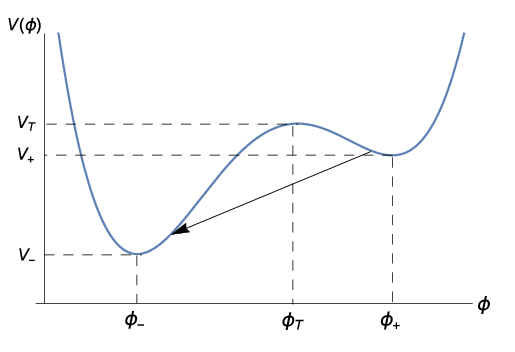
We are interested in the false vacuum decay initiated by the nucleation of a bubble of true vacuum within the false vacuum. This bubble nucleation occurs via quantum mechanical tunneling process, which can be described by an Euclidean bounce solution as discussed in [1]. We assume that the solution is -symmetric. Taking the ansatz of the metric
| (2.4) |
with being the metric of a unit 3-sphere, the equation of motion reads
| (2.5) | ||||
| (2.6) |
Here we also assumed that depends only on , and the dots represent the derivative with respect to . Using (2.5) and (2.6), we find
| (2.7) |
We can choose (2.5) and (2.7) as the independent set of equations, and we would like to solve this set of equations. The -symmetric bounce solution is topologically a 4-sphere, with vanishing size of at and :
| (2.8) |
To avoid the conical singularity at and , we require that behaves as
| (2.9) |
In semi-classical (small ) approximation, the tunneling rate per unit volume is written as
| (2.10) |
We will refer to as the “bounce factor”, which is determined by the on-shell action of the Euclidean the bounce solution, while the coefficient comes from the one-loop determinant around this solution. We assume that is of order , and we will focus on the computation of bounce factor in what follows. As shown in [1], the bounce factor is given by
| (2.11) |
where is the on-shell action for the bounce solution of (2.5) and (2.7)
| (2.12) |
while is the Euclidean action of the reference solution, in which the scalar field is sitting at the false vacuum . In this reference solution, the equation (2.7) for reduces to a simple harmonic oscillator equation
| (2.13) |
and the reference solution of false vacuum is easily obtained as
| (2.14) |
One can see that this reference solution obeys the regularity condition (2.9) at and with
| (2.15) |
The action of the reference solution at false vacuum is evaluated as
| (2.16) |
For general solution, eq.(2.7) can be seen as a harmonic oscillator with field dependent frequency. On the other hand, eq.(2.5) for the scalar field has a friction term proportional to , hence there is no simple way to find an integral of motion. Except for very special potentials [7, 8], we do not have analytic solutions of (2.5) and (2.7) for generic choice of potential. Instead, we will analyze the system of equations (2.5) and (2.7) numerically.
However, it turns out that this is not so straightforward as one might think. We are looking for a solution approaching
| (2.17) |
and obeying the regularity condition for the metric (2.9). One difficulty is that the value of at which the factor vanishes is not known a priori, and is determined by the solution itself. In other words, we can only know the value of after we solved the equations of motion (2.5) and (2.7), and the boundary condition at cannot be simply set from the beginning. This makes the construction of a regular solution a highly non-trivial problem. Another difficulty is that, in general the initial and the final values of the scalar field are different from the local minima of the potential
| (2.18) |
The existence of a regular solution is not guaranteed if we choose the initial value at random. As in the case of , we do not know the initial value of scalar field a priori. To find a regular solution, we have to fine-tune the initial value so that the solution obeying the conditions (2.9) and (2.18) exists.
The fact (2.18) that the tunneling does not necessarily start from the minimum of the potential has a natural interpretation as the effect of the thermal fluctuation due to the Gibbons-Hawking temperature associated with the de Sitter horizon [9]. A physical picture is that the scalar field first climbs up the potential from to by thermal fluctuation, then it tunnels through the barrier.
In [9, 10, 11, 12, 13], it is found that there are oscillating solutions crossing the top of the potential barrier times before settling down to . It is argued that as the number of oscillation increases becomes larger, which implies that the dominant contribution comes from the non-oscillating solution. Thus, in this paper we will consider the non-oscillating solution only.
The numerical study of bounce solution can be found in the literature [14, 15, 16, 17, 18, 19, 20, 21, 22], but the systematic study for various types of potential have not been performed, as far as we know. In this paper, we will consider two types of potentials, as simple examples. We should stress that the our numerical construction of solutions can be applied to arbitrary shape of the potential.
We find that as the initial value approaches the local maximum , the bounce factor of our solution is well approximated by the bounce factor of the Hawking-Moss (HM) tunneling [23],
| (2.19) |
corresponding to the solution sitting at the top of the barrier .
3 The thin-wall approximation
The thin-wall approximation requires a rapid transition of from to near the wall. It is argued in [1] that the thin-wall approximation is valid when the potential difference between the true vacuum and the false vacuum is small.
To compute the bounce factor in the thin-wall approximation, we divide the integration region into three parts: outside and inside of the bubble, and the contribution of the wall. In the thin-wall approximation, we can approximate that is sitting at the false vacuum outside the bubble. Thus the contribution outside the bubble is
| (3.1) |
Near the wall, we can neglect the friction term in (2.5)
| (3.2) |
and (2.5) becomes
| (3.3) |
This equation can be solved as:
| (3.4) |
Therefore, the contribution of the wall, , is given by
| (3.5) |
where is the bubble size and is the tension of the wall which is determined by the barrier between the false vacuum and the true vacuum. Inside the bubble, is sitting approximately at the true vacuum. For a constant , eq.(2.6) becomes
Therefore, eq.(2.12) is written as
| (3.6) |
Hence, the contribution of the inside of the bubble is
| (3.7) |
Adding the three contributions , , and , we obtain
| (3.8) |
The bubble size is determined by extremizing in (3.8)
| (3.9) |
from which is found to be
| (3.10) |
Plugging in (3.10) into (3.8), the bound factor in the thin-wall approximation is given by
| (3.11) |
4 Numerical Analysis
In this section, we construct the CdL instanton solution numerically for some scalar potentials, by solving the set of equations (2.5) and (2.7). Then we compute the bounce factor from this numerical solution and study the dependence of on the various parameters in the potential. As simple examples, we consider the -type potential and the -type periodic potential. They have natural cosmological and phenomenological applications. We should stress that our numerical approach can be applied to any shape of potential, say the potential with a negative mass-squared term (double-well potential).
To solve (2.5) and (2.7), we set the initial conditions of and as
| (4.1) |
There is one subtle point: To find a solution numerically, we have to introduce a regularization parameter for the initial value of the scale factor
| (4.2) |
so that the denominator in the friction term of (2.5) is non-zero at the initial value. We choose the value of the parameter as
| (4.3) |
Once we know the numerical bounce solution, we can numerically calculate the bounce factor by plugging the solution into (2.11). Then, we can compare this result with the thin-wall approximation (3.11) and the bounce factor of Hawking-Moss instanton (2.19).
4.1 potential
First, we consider the potential of the form
| (4.4) |
where is a mass parameter, and , and (4.4) are arbitrary parameters. This type of potential naturally appears from the open string tachyon living on unstable D-branes and it has an application to tachyon driven cosmology [25, 24]. We also added a term to make the true vacuum and false vacuum to have slightly different potential values. We will solve the set of equations (2.5) and (2.7) with this potential. In doing this, we set for definiteness.

We analyze the CdL tunneling rate by changing the parameters , and , which is equivalent to changing the values , and . To have the transition between two de Sitter vacua, we take the potential to be always positive: .
In this case, the false vacuum and the true vacuum correspond to . However, as discussed around (2.18) the scalar field in the bounce solution starts and ends at finite values. An example of the shape of the solution and are shown in Figure 3. From this figure, one can see that the actual solution of CdL instanton does not start and end at , and the initial and the final values of the scalar field are some finite values. The scale factor is not much different from the reference solution in (2.14), in this example.
 |
 |
We calculate and for various values of with fixed potential difference and . In other words, we change the off-set of the potential in (4.4) without changing the shape of the potential parametrized by .
 |
 |
In Figure 4, we show the plot of and as a function of . From Figure 4, one can see that decreases as increases, and approaches for large . This shows that the initial value of scalar field approaches the top of the potential barrier when becomes large. On the other hand, approaches when is small. Therefore, the probability of the CdL tunneling is controlled by the off-set scale of the potential in this setup.
This suggests the following picture: When the potential height becomes large the tunneling probability increases, and the universe is very mobile and tends to move around the landscape of vacua. On the other hand, as the energy scale becomes small, the tunneling to other vacua is highly suppressed and the universe is bound to one of the vacua. This is analogous to the metal-insulator transition in the condensed-matter physics. In the next subsection, we will consider the tunneling rate in the periodic potential. The analogy to the electron in the crystal is more appropriate in the example of periodic potential, as advocated in [4].
4.2 Periodic Potential
Next, we analyze the tunneling rate in the case of periodic potential
| (4.5) |
where is some non-perturbatively generated scale, is the axion decay constant, and are arbitrary parameters. This type of potential was first introduced to solve the strong CP problem by promoting the theta-angle of QCD to a dynamical field, called axion [26, 27]. This type of axionic scalar fields is considered in many contexts, beyond the original QCD axion. In particular, axionic fields appear naturally in string compactifications from the extra dimensional components of the anti-symmetric tensor fields in string theory.
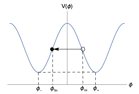
 |
 |
The procedure of solving the equations of motion (2.5) and (2.6) are the same as the previous subsection. Using the numerical solution of and , we evaluate the bounce factor for various values of the parameters in (4.5).
 |
 |
First, by fixing and , , we calculate and for various values of the axion decay constant . Figure 7 shows the plot of (or ) against (left figure) and (right figure). From the left figure of Fig. 7, one can see that both and become large as increases. Also, this figure shows that the thin-wall approximation gets worse when becomes large. We also find that when increases, the initial value of the potential approaches the value of the potential at the top of the barrier. This implies that the bounce factor approaches the Hawking-Moss value for large . Interestingly, in order for the regular solution to exist, the range of allowed is restricted
| (4.6) |
since the initial value of the potential is bounded from both above and below:
| (4.7) |
The bounds and in (4.6) correspond to the limit where approaches and , respectively:
| (4.8) |
For the parameter choice in Figure 7, we find that the allowed range of is . It would be interesting to understand the cosmological implication (if any) of this bound on the axion decay constant.
Next, by fixing , we calculate the bounce factor by varying the axion decay constant for various values of .

Figure 8 and Figure 9 are the plot against with various values of or , respectively. From those figures, one can see that becomes large as the energy scale of the axion potential becomes small. From Figure 9, we can also read off the behavior of that when the potential scale is reduced by a factor of , the bounce factor roughly becomes times larger.
This behavior suggests the analogy with the electrons in a crystal as mentioned at the end of the previous subsection. As the energy scale of the axion potential is lowered, the tunneling probability becomes negligibly small and the universe is “tight-binded” to one of the vacua. On the other hand, as the energy scale increases, the wavefunction of the universe spreads over the landscape of vacua as a Bloch-wave in analogy with the conducting electrons in a metal [4]. From Figure 8, we also notice that the allowed range of (4.6) changes as we change the energy scale of axion potential . In this example, the maximum of the allowed axion decay constant never exceeds the Planck scale .

5 Conclusion and Discussion
In the paper, we numerically analyzed the false vacuum decay in the presence of gravity described by the CdL instanton, and studied the dependence of the bounce factor in (2.11) on the various parameters in the scalar potential. We also numerically calculated the bounce factor in the thin-wall approximation, and compared with . We find that when the initial value of the potential becomes large the thin-wall approximation gets worse. Therefore, the thin-wall approximation can only be trusted in the case that is close to the false vacuum value , and the difference of the potential between the false vacuum and the true vacuum is small .
As simple examples, we considered the potential and the axionic periodic potential, where both types of potential have an interesting application to cosmology. Especially, the periodic axionic potentials have been considered in many cosmological models, such as natural inflations [28] and the cosmic landscape in superstring compactifications. We found that the CdL tunneling rate of this axionic potential depends on the energy scale and the axion decay constant in (4.5). We find that the tunneling probability is highly suppressed when becomes small. From the observation we know that the cosmological constant of our universe is very small, hence the value of the scalar potential of our current universe is expected to be at very low energy, hence the tunneling to other vacuum can be safely ignored in today’s universe. On the other hand, the tunneling effect cannot be ignored when we consider the physics around the Planck scale. We also find that the axion decay constant is bounded both from above and below (4.6), in order for the smooth tunneling solution to exist. It would be interesting to see if this bound has some cosmological implications.
References
- [1] S. R. Coleman and F. De Luccia, “Gravitational Effects on and of Vacuum Decay,” Phys. Rev. D 21, 3305 (1980). doi:10.1103/PhysRevD.21.3305
- [2] S. R. Coleman, “The Fate of the False Vacuum. 1. Semiclassical Theory,” Phys. Rev. D 15, 2929 (1977) [Phys. Rev. D 16, 1248 (1977)]. doi:10.1103/PhysRevD.15.2929, 10.1103/PhysRevD.16.1248
- [3] L. Susskind, “The Anthropic landscape of string theory,” In *Carr, Bernard (ed.): Universe or multiverse?* 247-266 [hep-th/0302219].
- [4] S.-H. Henry Tye, D. Wohns and Y. Zhang, “Coleman-de Luccia Tunneling and the Gibbons-Hawking Temperature,” Int. J. Mod. Phys. A 25, 1019 (2010) doi:10.1142/S0217751X10047981 [arXiv:0811.3753 [hep-th]].
- [5] B. H. Lee and W. Lee, “Vacuum bubbles in a de Sitter background and black hole pair creation,” Class. Quant. Grav. 26, 225002 (2009) doi:10.1088/0264-9381/26/22/225002 [arXiv:0809.4907 [hep-th]].
- [6] B. H. Lee, C. H. Lee, W. Lee and C. Oh, “Instanton solutions mediating tunneling between the degenerate vacua in curved space,” Phys. Rev. D 82, 024019 (2010) doi:10.1103/PhysRevD.82.024019 [arXiv:0910.1653 [hep-th]].
- [7] X. Dong and D. Harlow, “Analytic Coleman-De Luccia Geometries,” JCAP 1111, 044 (2011) doi:10.1088/1475-7516/2011/11/044 [arXiv:1109.0011 [hep-th]].
- [8] S. Kanno and J. Soda, “Exact Coleman-de Luccia Instantons,” Int. J. Mod. Phys. D 21, 1250040 (2012) doi:10.1142/S021827181250040X [arXiv:1111.0720 [hep-th]].
- [9] J. C. Hackworth and E. J. Weinberg, “Oscillating bounce solutions and vacuum tunneling in de Sitter spacetime,” Phys. Rev. D 71, 044014 (2005) doi:10.1103/PhysRevD.71.044014 [hep-th/0410142].
- [10] T. Banks, “Heretics of the false vacuum: Gravitational effects on and of vacuum decay. 2.,” hep-th/0211160.
- [11] G. Lavrelashvili, “The Number of negative modes of the oscillating bounces,” Phys. Rev. D 73, 083513 (2006) doi:10.1103/PhysRevD.73.083513 [gr-qc/0602039].
- [12] B. H. Lee, C. H. Lee, W. Lee and C. Oh, “Oscillating instanton solutions in curved space,” Phys. Rev. D 85, 024022 (2012) doi:10.1103/PhysRevD.85.024022 [arXiv:1106.5865 [hep-th]].
- [13] B. H. Lee, W. Lee, D. Ro and D. h. Yeom, “Oscillating Fubini instantons in curved space,” Phys. Rev. D 91, no. 12, 124044 (2015) doi:10.1103/PhysRevD.91.124044 [arXiv:1409.3935 [hep-th]].
- [14] B. H. Lee, C. H. Lee, W. Lee and C. Oh, “The nucleation of false vacuum bubbles with compact geometries,” Int. J. Mod. Phys. A 30, no. 18n19, 1550110 (2015) doi:10.1142/S0217751X15501109 [arXiv:1311.4279 [hep-th]].
- [15] D. A. Samuel and W. A. Hiscock, “Effect of gravity on false vacuum decay rates for O(4) symmetric bubble nucleation,” Phys. Rev. D 44, 3052 (1991). doi:10.1103/PhysRevD.44.3052
- [16] D. A. Samuel and W. A. Hiscock, “’Thin wall’ approximations to vacuum decay rates,” Phys. Lett. B 261, 251 (1991). doi:10.1016/0370-2693(91)90323-I
- [17] Y. l. Zhang, R. Saito, D. h. Yeom and M. Sasaki, “Coleman-de Luccia instanton in dRGT massive gravity,” JCAP 1402, 022 (2014) doi:10.1088/1475-7516/2014/02/022 [arXiv:1312.0709 [hep-th]].
- [18] S. Kachru, R. Kallosh, A. D. Linde and S. P. Trivedi, “De Sitter vacua in string theory,” Phys. Rev. D 68, 046005 (2003) doi:10.1103/PhysRevD.68.046005 [hep-th/0301240].
- [19] R. Casadio and A. Orlandi, “Bubble dynamics: (nucleating) radiation inside dust,” Phys. Rev. D 84, 024006 (2011) doi:10.1103/PhysRevD.84.024006 [arXiv:1105.5497 [gr-qc]].
- [20] G. Isidori, V. S. Rychkov, A. Strumia and N. Tetradis, “Gravitational corrections to standard model vacuum decay,” Phys. Rev. D 77, 025034 (2008) doi:10.1103/PhysRevD.77.025034 [arXiv:0712.0242 [hep-ph]].
- [21] M. Artymowski, Z. Lalak and M. Lewicki, “Inflationary scenarios in Starobinsky model with higher order corrections,” JCAP 1506, 032 (2015) doi:10.1088/1475-7516/2015/06/032 [arXiv:1502.01371 [hep-th]].
- [22] J. R. Espinosa, J. F. Fortin and M. Trépanier, “Consistency of Scalar Potentials from Quantum de Sitter Space,” arXiv:1508.05343 [hep-th].
- [23] S. W. Hawking and I. G. Moss, “Supercooled Phase Transitions in the Very Early Universe,” Phys. Lett. B 110, 35 (1982). doi:10.1016/0370-2693(82)90946-7
- [24] A. Sen, “Remarks on tachyon driven cosmology,” Phys. Scripta T 117, 70 (2005) [hep-th/0312153].
- [25] A. Sen, “Time and tachyon,” Int. J. Mod. Phys. A 18, 4869 (2003) doi:10.1142/S0217751X03015313 [hep-th/0209122].
- [26] R. D. Peccei and H. R. Quinn, “CP Conservation in the Presence of Instantons,” Phys. Rev. Lett. 38, 1440 (1977). doi:10.1103/PhysRevLett.38.1440
- [27] R. D. Peccei and H. R. Quinn, “Constraints Imposed by CP Conservation in the Presence of Instantons,” Phys. Rev. D 16, 1791 (1977). doi:10.1103/PhysRevD.16.1791
- [28] K. Freese, J. A. Frieman and A. V. Olinto, “Natural inflation with pseudo - Nambu-Goldstone bosons,” Phys. Rev. Lett. 65, 3233 (1990). doi:10.1103/PhysRevLett.65.3233