-exponential behavior of expected aggregated supply curves in deregulated electricity markets
Abstract.
It has been observed that the expected aggregated supply curves of the colombian electricity market present -exponential behavior. The purpose of this article is to present evidence supporting the fact that -exponentiality is already present in the expected aggregated supply curve of certain extremely simple idealized deregulated electricity markets where illegal interaction among competing firms is precluded.
1. Introduction
In the last two decades, more and more countries have adopted a deregulated electricity market policy. In these countries, an inverse
auction mechanism is implemented each day in order to determine, for the next day, which generating units will be operating, how much electricity
will be supplied by each one of them, and its unitary price. Since the electrical sector is of utmost importance in any country’s economy, it is important
to understand various aspects of the corresponding market. One of such aspects is the expected aggregated supply curve, which will be refered to as supply curve for short, resulting from the competition among generating firms.
It has been observed that the supply curve for each of the years in the period -, in the colombian electricity market (a deregulated one),
are well fitted by suitably scaled -exponential curves, where the values of vary from year to year and are generally different from [4].
The presence of -exponential behavior or -deformed behavior in general, has been observed in quantities arising in similar contexts. In [1] certain quantities
associated to the Czech Republic public procurement market (an auction type market), for the period -, are analyzed. Specifically, those authors look at the behavior of three quantities,
namely, the probability that a contract has bidders or more, the probability that a public procurement selling agent makes euros or more during the observed period (-), and the
probability that a contracting authority spends or more euros during the observed period, as functions of in the first case, and in the second and third cases.
They observe that the first function is very well approximated by certain
exponential, while the second and third functions, are very well approximated by certain power functions.
Now, exponential functions and power functions correspond to -exponentials, with in the first case and in the second one.
In [2] the probability distribution of certain quantities associated to the opening call auctions in the chinese stock market are studied. In particular, it is shown that the probability distribution of order sizes is well fitted by
certain -Gamma function.
Even though the presence of -deformed behavior, with , may be taken as evidence of complexity in the dynamics governing the corresponding processes, illegal interaction between participants and so on, it is still valid to ask whether there is already -deformed behavior, with , in situations having low complexity and complete transparency.
In this article we study the presence of -deformed behavior in the seemingly most simple situation arising in deregulated electricity markets. Concretely, we consider an electricity market composed of a number of generating firms, each one having a single generating set capable of supplying (after normalization) one electricity unit per day whose production cost is assumed (after normalization) to be zero. In addition, the demand is a discrete random variable whose probability distribution is known by all firms. As was mentioned before, the firms compete each day in a reverse auction in order to be selected as an electricity supplier for the next day. This simple market can be thought as a repeated game in the framework of classical game theory, i.e. one in which players are rational and have complete knowledge of the game structure. Therefore, we assume that players place their bids according to a Nash equilibrium. After calculating and solving a differential equation whose solution is the unique symmetric Nash equilibrium possesed by this game, we estimate the supply curve by simulating repetitions of this game. We observed that for various background probability distributions for the demand, and a range of numbers of generating firms, the supply curves are well fitted by -exponential curves, usually with , and that for fixed background distribution, the value of gets closer to as the number of generating firms increases. Towards the end of the paper we propose a plausible explanation for these phenomena.
2. General model
In this section we closely follow [3]. We assume that the electricity generating system is formed by electricity generating firms , and that each firm has generating units or sets . Let be the total number of sets of the whole generation system. Each set can produce at most electrity units per day and has a cost function , assigning to each , the cost of producing electricity units using . Let be the total daily capacity of the generating system. We assume that the amount of electricity demanded by the consumers in one day is a random variable that distributes according to certain cumulative distribution function supported on some interval . Policies for the market demand that firms can only offer unitary prices lying within certain interval . It is assumed that all the information above is common knowledge. The mechanism by which electricity is bought is the following. Each day (day ), each secretely submits a vector to a coordinating entity, expressing its willingness to produce the next day (day ), using set , any amount of electricity in the interval , and to sell it at a unitary price of . At this point we emphasize the fact that the generators decide on their price vectors knowing the distribution but without knowing the particular value it takes the next day. Once the coordinating entity receives all these vectors, it chooses a ranking of the prices, i.e. a bijective function such that whenever . Notice that this choice is not unique whenever there exist pairs such that . More precisely, if is the partition induced on the set by the equivalence relation iff , the number of choices is . Here denotes the number of elements of the set . This number will be denoted by . The coordinator randomly selects one of the possible rankings according to a uniform distribution, i.e. with probability . Once a ranking is chosen, the coordinator looks at the actual demand of electricity for day . It is useful at this point to rename the generating units and all the entities associated to them, according to their rank, i.e. to denote the unit by , by , and so on. The coordinator considers the numbers and for , and determines . Then the coordinator dictates that on day , each unit with will supply its full capacity , that unit will supply units of electricity, and that each unit of electricity will be paid at price . It is understood that units with will not supply any electricity and therefore will not receive any payment. The utility for firm is therefore given by
| (2.1) |
where is if belongs to firm and is zero otherwise.
Since we will consider the case when (i) each generator has a single generating unit , (ii) each generating unit has capacity , (iii) all cost functions are , (iv) the demand is a discrete random variable taking values , and (v) ; these five conditions will be assumed to hold for the rest of the paper. In this case it is important to slightly modify our notation. Instead of writing we will write , respectively. The renaming of units and associated entities induced by a ranking keeps being the same as before, i.e. are renamed as , respectively.
The assumption that firms want to maximize their utilities, naturally leads to the interpretation of the whole situation as the repetition of a three stage game: first, firms choose their prices in the interval , then nature chooses a value for the demand according to some probability distribution , , and finally the coordinator makes the dispatchment according to the rules already explained. Notice that the latter step involves a random choice in order to resolve ties. The utilities for each firm depend on the prices being offered by all firms, the value taken by the demand and the particular ranking chosen by the coordinator. This game can thought as a random experiment, whose sample space is
| (2.2) |
with probability density function (pdf) having the form
| (2.3) |
Here are some pdf’s. In this setting the utility functions become random variables. The functions according to which firms choose their prices, form a Nash equilibrium, if for each , the expected utility of firm ,
| (2.4) |
for any other pdf . It is equivalent but much easier to work with the corresponding cummulative distribution functions . These will be nondecreasing functions defined on , having value at and at , and admitting (jump) discontinuities.
According to proposition 6 in [3] is a (symmetric) Nash equilibrium if and only if is a nondrecreasing function defined on a closed interval with , such that , , and satisfying the differential equation
| (2.5) |
where
and
We remark that this differential equation derives from the general fact that a profile of mixed strategies is a Nash equilibrium if and only if for each , the (expected) profit of firm assuming that it plays the pure strategy while any other firm plays according to , is independent of . We observe that this differential equation can be solved by separation of variables.
3. Experiments and results
In order to survey the behavior of supply curves in general, we wrote routines in Mathematica 10.1 and used them for testing various scenarios. The main routine, called GranProgramaP, assumes and for given distribution of background demand, and positive integers and , it first determines the differential equation 2.5, finds the solution to this differential equation subject to the condition , and then, for each , it produces an -vector , by first making independent (random) choices of numbers in the interval according to , sorting these numbers in increasing order, and finally computing the average -vector . Finally, the Mathematica command NMinimize is applied to find, among the curves with , , and whenever , one that (approximately) minimizes the quadratic error
Next we present the considered scenarios and the results obtained in each case. The reason for the kind of experiment performed in each of these scenarios is clarified in section 4. The following four experiments have the following common structure. We assume a market with generating firms, each of them capable of producing units per day at production cost zero, and with demand being a discrete random variable taking values for , with probability
for a fixed probability distribution supported on the interval . We refer to as the background distribution for the demand. This is of course equivalent to a market with generating firms, each of them capable of producing unit per day at production cost zero, and with demand being a discrete random variable taking values , with probability
So the experiments only differ by the choice of background distribution. In all four experiments we set and for NMinize we selected the RandomSearch method with search points.
3.1. Experiment 1
In this experiment we took as background distribution for the demand. Table 1 shows the results obtained for values of from to .
| Uniform demand | ||||
|---|---|---|---|---|
| quadratic error | ||||
| 5 | 0.863233 | 2.9002 | 0.823226 | 0.0193731 |
| 6 | 0.89449 | 1.2304 | 0.859379 | 0.0672908 |
| 7 | 0.892939 | 0.437755 | 0.980874 | 0.00743362 |
| 8 | 0.916562 | 0.183676 | 0.972093 | 0.00345962 |
| 9 | 0.933164 | 0.0836263 | 0.955353 | 0.00345632 |
| 10 | 0.93709 | 0.0322543 | 0.997464 | 0.00232163 |
| 11 | 0.939185 | 0.0121861 | 1.04244 | 0.00379461 |
| 12 | 0.947345 | 0.00562502 | 1.02362 | 0.00259078 |
| 13 | 0.943343 | 0.00147738 | 1.1462 | 0.0115656 |
| 14 | 0.957351 | 0.000978965 | 1.02787 | 0.00465776 |
| 15 | 0.962617 | 0.000435722 | 1.01207 | 0.0013087 |
| 16 | 0.987828 | 0.000814185 | 0.765452 | 0.0169305 |
| 17 | 0.969912 | 0.000107791 | 0.972005 | 0.00665632 |
| 18 | 0.950759 | 1.4119 | 0.0184282 | |
| 19 | 0.968327 | 0.0000111811 | 1.06863 | 0.00827299 |
| 20 | 0.973942 | 0.988244 | 0.00439083 | |
| 21 | 0.991221 | 0.0000229271 | 0.76225 | 0.0286424 |
| 22 | 0.982056 | 0.908473 | 0.0226434 | |
| 23 | 0.984581 | 0.882888 | 0.0220357 | |
| 24 | 0.992261 | 0.769326 | 0.0998453 | |
| 25 | 0.995941 | 0.717738 | 0.0957674 | |
| 26 | 0.993057 | 0.761542 | 0.087408 | |
| 27 | 1.0081 | 0.596923 | 0.154767 | |
| 28 | 1.01065 | 0.575789 | 0.199678 | |
3.2. Experiment 2
In this experiment we took as background distribution for the demand. Table 2 shows the results obtained for values of from to .
| Demand’s f.d.p based on , | ||||
|---|---|---|---|---|
| quadratic error | ||||
| 5 | 0.786277 | 9.24399 | 0.562637 | 0.000517729 |
| 6 | 0.848111 | 4.08727 | 0.632552 | 0.0713172 |
| 7 | 0.882261 | 1.72287 | 0.691693 | 0.0499626 |
| 8 | 0.905359 | 0.724865 | 0.738601 | 0.012073 |
| 9 | 0.910659 | 0.289822 | 0.805672 | 0.00154287 |
| 10 | 0.923683 | 0.114552 | 0.843706 | 0.0121201 |
| 11 | 0.940745 | 0.0609441 | 0.80781 | 0.0103708 |
| 12 | 0.952511 | 0.0259056 | 0.810255 | 0.00760159 |
| 13 | 0.953217 | 0.0102512 | 0.850152 | 0.00430776 |
| 14 | 0.962814 | 0.00485199 | 0.829615 | 0.0294654 |
| 15 | 0.959879 | 0.00173207 | 0.888678 | 0.0151036 |
| 16 | 0.956018 | 0.000481014 | 0.983035 | 0.00436682 |
| 17 | 0.962618 | 0.000285168 | 0.934857 | 0.0044448 |
| 18 | 0.967372 | 0.000148451 | 0.910055 | 0.0162562 |
| 19 | 0.974735 | 0.0000893455 | 0.85638 | 0.00924199 |
| 20 | 0.973182 | 0.0000324616 | 0.896141 | 0.0112569 |
| 21 | 0.962477 | 1.14381 | 0.0111554 | |
| 22 | 0.990649 | 0.0000259162 | 0.725679 | 0.0354996 |
| 23 | 0.975639 | 0.938534 | 0.0101328 | |
| 24 | 0.975775 | 0.955251 | 0.0344693 | |
| 25 | 0.983022 | 0.850342 | 0.0896586 | |
| 26 | 0.997108 | 0.667209 | 0.0643818 | |
| 27 | 1.00178 | 0.63024 | 0.134193 | |
| 28 | 0.991328 | 0.750202 | 0.0612747 | |
3.3. Experiment 3
In this experiment we took as background distribution for the demand. Table 2 shows the results obtained for values of from to .
| Demand’s f.d.p based on , | ||||
|---|---|---|---|---|
| quadratic error | ||||
| 5 | 1.09464 | 0.206346 | 0.848798 | 0.0024282 |
| 6 | 1.09723 | 0.0711591 | 0.798572 | 0.00177619 |
| 7 | 1.10279 | 0.0319655 | 0.730883 | 0.00488975 |
| 8 | 1.11106 | 0.0156945 | 0.660128 | 0.00499712 |
| 9 | 1.09178 | 0.00541504 | 0.679568 | 0.00123698 |
| 10 | 1.09736 | 0.00281438 | 0.625793 | 0.000942782 |
| 11 | 1.09776 | 0.00163252 | 0.58577 | 0.000979379 |
| 12 | 1.06551 | 0.000271507 | 0.690339 | 0.000269798 |
| 13 | 1.0952 | 0.000422896 | 0.538375 | 0.00126523 |
| 14 | 1.08674 | 0.000198589 | 0.538884 | 0.000486154 |
| 15 | 1.09073 | 0.00012446 | 0.502844 | 0.00021681 |
| 16 | 1.06933 | 0.0000260694 | 0.565947 | 0.000614531 |
| 17 | 1.08805 | 0.0000376827 | 0.471669 | 0.000287819 |
| 18 | 1.08563 | 0.0000213679 | 0.460938 | 0.000232498 |
| 19 | 1.09183 | 0.0000198484 | 0.422582 | 0.00157232 |
| 20 | 1.10914 | 0.0000282786 | 0.36162 | 0.00176623 |
| 21 | 1.0921 | 0.392186 | 0.000280447 | |
| 22 | 1.09542 | 0.368959 | 0.000318908 | |
| 23 | 1.09237 | 0.364318 | 0.00249175 | |
| 24 | 1.08245 | 0.383466 | 0.000381974 | |
| 25 | 1.09711 | 0.32872 | 0.00305721 | |
| 26 | 1.08742 | 0.344124 | 0.00312855 | |
| 27 | 1.11564 | 0.269265 | 0.00625656 | |
| 28 | 1.11006 | 0.271704 | 0.00357036 | |
3.4. Experiment 4
So far we have considered background demands distributed according to power-like functions. It is important to experiment with more general background distributions for the demand. Let us consider for instance a background demand distributed as some randomly selected piecewise constant function whose graph is depicted in Figure 1.
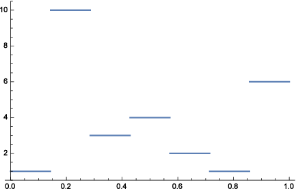
Table 4 shows the results obtained for values of from to .
| Demand’s f.d.p based on , | ||||
|---|---|---|---|---|
| quadratic error | ||||
| 5 | 0.72133 | 2.954427 | 1.129140 | 0.4091208 |
| 6 | 0.67358 | 0.821282 | 1.861038 | 1.8020197 |
| 7 | 0.64121 | 0.038771 | 6.119756 | 2.8822813 |
| 8 | 0.69959 | 0.005481 | 7.269161 | 1.2973836 |
| 9 | 0.73581 | 0.000718 | 8.862518 | 1.39342351 |
| 10 | 0.77651 | 0.000579 | 5.932255 | 0.6524641 |
| 11 | 0.80561 | 0.000245 | 5.070716 | 0.4075098 |
| 12 | 0.83691 | 0.000347 | 3.309873 | 0.0719115 |
| 13 | 0.85802 | 0.000301 | 2.624487 | 0.0562562 |
| 14 | 0.87835 | 0.000241 | 2.143395 | 0.1501309 |
| 15 | 0.90866 | 0.000540 | 1.418274 | 0.2352072 |
| 16 | 0.92360 | 0.000395 | 1.247219 | 0.2155978 |
| 17 | 0.94694 | 0.000562 | 0.961471 | 0.26144589 |
| 18 | 0.97006 | 0.000738 | 0.762271 | 0.2988319 |
| 19 | 0.98948 | 0.000945 | 0.628611 | 0.2476883 |
| 20 | 0.99752 | 0.000670 | 0.587217 | 0.2163773 |
| 21 | 1.01654 | 0.000856 | 0.491904 | 0.1813817 |
| 22 | 1.02361 | 0.000688 | 0.460020 | 0.2267202 |
| 23 | 1.02211 | 0.000373 | 0.463638 | 0.2033697 |
| 24 | 1.02958 | 0.000297 | 0.432238 | 0.1293418 |
| 25 | 1.02354 | 0.000119 | 0.457114 | 0.0546924 |
| 26 | 1.03403 | 0.000130 | 0.409306 | 0.0751101 |
| 27 | 1.04037 | 0.000121 | 0.381030 | 0.0664762 |
| 28 | 1.03368 | 0.000044 | 0.405377 | 0.0281123 |
4. Analysis of results and conclusions
The results obtained in the previous section strongly indicate the presence of -exponential behavior, with , of the supply curve in the various tested scenarios. The quadratic errors oscillated between and in experiment 1, between and in experiment 2, between and in experiment 3, and between and in experiment 4. These errors are very small in comparison with the quantities being approximated. It is important to observe that the emergence of -exponential behavior in these experiments cannot be due to any illegal behavior, since the mathematical model assumes that prices are chosen independently by the generating firms. Figure 2

insinuates an interesting tendency: for fixed background demand, the value of gets closer to as gets larger. These observations suggest the following interpretation. When the number of competing firms is small, we can consider each one of them as a maximally strong coalition of a large number of minifirms. This allows us to consider the small number of competing firms as a huge number of competing firms divided into groups so that firms belonging to one group strongly interact mutually and firms belonging to different groups do not interact. Therefore getting larger has the effect of breaking coalitions, reducing in this way the level of interaction, thus making closer to . We infer that as gets larger, the market gets closer to a perfect competition market. This suggests the possibility of modeling these markets as statistical mechanical systems having nontrivial particle interaction [5], and justifying in this way the presence of -exponential behavior in this setting.
References
- [1] Kristoufek, L., and Skuhrovec, J. (2012). Exponential and power laws in public procurement markets. EPL (Europhysics Letters), 99(2), 28005.
- [2] Gu, G. F., Ren, F., Ni, X. H., Chen, W., and Zhou, W. X. (2010). Empirical regularities of opening call auction in Chinese stock market. Physica A: Statistical Mechanics and its Applications, 389(2), 278-286.
- [3] von der Fehr, Nils-Henrik Mørch, and David Harbord. ”Spot market competition in the UK electricity industry.” The Economic Journal (1993): 531-546.
- [4] Private communication with prof. Gabriel Loaiza.
- [5] Tsallis, C. (2011). The nonadditive entropy Sq and its applications in physics and elsewhere: Some remarks. Entropy, 13(10), 1765-1804..