跳到论文正文
W Papers独立论文阅读器 arXiv:1601.07411 论文正文 计算阅读时间 · 0%
引用这篇论文根据当前论文元数据生成,正式投稿前建议核对。


License: arXiv.org perpetual non-exclusive license
arXiv:1601.07411v1 [cond-mat.stat-mech] 27 Jan 2016

∎

Error Analysis of Modified Langevin Dynamics

Journal: my journal
Stephane Redon†    Gabriel Stoltz‡    Zofia Trstanova† Affiliation: Inria - Univ. Grenoble Alpes, LJK, F-38000 Grenoble, France
CNRS, LJK, F-38000 Grenoble, France
E-mail: zofia.trstanova@inria.fr Affiliation: Université Paris-Est, CERMICS (ENPC), INRIA, F-77455 Marne-la-Vallée, France
Received: date / Accepted: date
Abstract

We consider Langevin dynamics associated with a modified kinetic energy vanishing for small momenta. This allows us to freeze slow particles, and hence avoid the re-computation of inter-particle forces, which leads to computational gains. On the other hand, the statistical error may increase since there are a priori more correlations in time. The aim of this work is first to prove the ergodicity of the modified Langevin dynamics (which fails to be hypoelliptic), and next to analyze how the asymptotic variance on ergodic averages depends on the parameters of the modified kinetic energy. Numerical results illustrate the approach, both for low-dimensional systems where we resort to a Galerkin approximation of the generator, and for more realistic systems using Monte Carlo simulations.

Keywords: 
Langevin dynamics Variance reduction Ergodicity Functional estimates Linear response

1 Introduction

A fundamental purpose of molecular simulation is the computation of macroscopic quantities, typically through averages of functions of the variables of the system with respect to a given probability measure μ\mu, which defines the macroscopic state of the system. In the most common setting, the probability measure μ\mu with respect to which averages are computed corresponds to the canonical ensemble (see for instance Tuckerman (2010)). Its distribution is defined by the Boltzmann-Gibbs density, which models the configurations of a conservative system in contact with a heat bath at fixed temperature. Numerically, high-dimensional averages with respect to μ\mu are often approximated as ergodic averages over realizations of appropriate stochastic differential equations (SDEs):

limt→∞A^t=𝔼μ​(A)a.s.,A^t:=1t​∫0tA⁡(ps,qs)​𝑑s.\lim_{t\rightarrow\infty}\hat{A}_{t}=\mathbb{E}_{\mu}(A)\quad\text{a.s.},\qquad\hat{A}_{t}:=\frac{1}{t}\int_{0}^{t}A(p_{s},q_{s})\,ds\,. (1)

A typical dynamics to this end is the Langevin dynamics

{d​qt=M−1​pt​d​t,d​pt=−∇V​(qt)​d​t−γ​M−1​pt​d​t+2​γβ​d​Wt,\left\{\begin{aligned} \displaystyle dq_{t}&=M^{-1}p_{t}\,dt,\\ \displaystyle dp_{t}&=-\nabla V(q_{t})\,dt-\gamma M^{-1}p_{t}\,dt+\sqrt{\frac{2\gamma}{\beta}}\,dW_{t}\,,\end{aligned}\right. (2)

where d​WtdW_{t} is a standard Wiener process, VV the potential energy function, γ>0\gamma>0 a friction coefficient, MM the mass matrix of the system, and β\beta is proportional to the inverse temperature (see Section 2 for more precise definitions). For references on the ergodicity of Langevin dynamics, we refer the reader to Talay (2002) and Mattingly et al. (2002), for instance.

There are two main sources of error in the computation of average properties such as 𝔼μ​(A)\mathbb{E}_{\mu}(A) through time averages as in (1): (i) a systematic bias (or perfect sampling bias) related to the use of a discretization method for the SDEs (and usually proportional to a power of the integration step size Δ​t\Delta t), and (ii) statistical errors, due to the finite lengths of the sampling paths involved and the underlying variance of the random variables. The first point was studied in Leimkuhler et al. (2015) for standard Langevin dynamics. Our focus in this work is on the statistical error.

Statistical errors may be large when the dynamics is metastable, i.e. when the system remains trapped for a very long time in some region of the configuration space (called a metastable region) before hopping to another metastable region. Metastability implies that the convergence of averages over trajectories is very slow, and that transitions between metastable regions (which are typically the events of interest at the macroscopic level) are very rare. In fact, metastability arises from the multi-modality of the probability measure sampled by the dynamics. We refer for instance to Lelièvre (2013) for a review on ways to quantify the metastability of sampling dynamics. There are various strategies to reduce the variance of time averages by reducing the metastability. The most famous one is importance sampling: the potential energy function VV is modified by an additional term V~\widetilde{V} so that the Langevin dynamics associated with V+V~V+\widetilde{V} is less metastable. An automatic way of doing so is to consider a so-called reaction coordinate, and define V~\widetilde{V} as the opposite of the associated free energy (see Lelièvre et al. (2010); Lelièvre and Stoltz (2015) for further precisions).

We explore here an alternative path, which consists in modifying the kinetic energy rather than the potential energy. Indeed, recall that the difficult part in sampling the canonical measure is in sampling positions (see Section 2 for a more precise discussion of this point). There is therefore some freedom in the choice of the kinetic energy if the goal is to compute average properties.

Previous works in this direction focused on changing the mass matrix in order to increase the time steps used in the simulation (see e.g. Bennett (1975); Plechac and Rousset (2010)). The mathematical analysis we provide is inspired by a recent work by Artemova and Redon (2012) where the kinetic energy of each particle is more drastically modified: it is set to 0 when the particle’s momenta are small, while it remains unchanged for larger momenta. In such adaptively restrained (AR) simulations, particles may become temporarily frozen, while their momenta may continue to evolve. Since, in many cases, inter-particle forces only depend on relative particle positions, and hence do not have to be updated when particles are frozen, adaptively restrained particle simulations may yield a significant algorithmic speed-up SalgoS_{\rm algo} when a sufficiently large number of particles are frozen at each time step (or, more generally, when inter-particle distances remain constant and particle forces are expressed in local reference frames). This has been demonstrated in several contexts, e.g. for modeling hydrocarbon systems (Bosson et al. (2012)), proteins (Rossi et al. (2007)), and for electronic structure calculations (Bosson et al. (2013)).

Unfortunately, freezing particles even temporarily may make iterates more correlated, which may translate into an increase of the statistical error σmod2\sigma^{2}_{\rm mod} observed for modified Langevin dynamics, compared to the statistical error σstd2\sigma_{\rm std}^{2} observed for standard Langevin dynamics. The actual speed-up of the method, in terms of the total wall-clock time needed to achieve a given precision in the estimation of an observable, should therefore be expressed as:

Sactual=Salgo​σstd2σmod2.S_{\rm actual}=S_{\rm algo}\frac{\sigma^{2}_{\rm std}}{\sigma^{2}_{\rm mod}}\,. (3)

Our aim here is thus to quantify the increase in the variance as a function of the parameters of the modified kinetic energy. In fact, a first task is to prove that the Langevin dynamics with modified kinetic energy is indeed ergodic, and that the variance is well defined. This is unclear at first sight since the modified dynamics fails to be hypoelliptic (see the discussion in Section 3.1).

This article is organized as follows. In Section 2, we introduce the modified Langevin dynamics we consider, and present the particular case of the AR-Langevin dynamic. The ergodicity of these dynamics is proved in Section 3, both in terms of almost-sure convergence of time averages along a single realization, and in terms of the law of the process. We also provide a result on the regularity of the evolution semi-group, adapted from similar estimates for standard Langevin dynamics in  Talay (2002). Such estimates allow us to analyze the statistical error in Section 4. We state in particular a Central Limit Theorem for A^t\widehat{A}_{t}, and perform a perturbative study of the asymptotic variance of the AR-Langevin dynamics in some limiting regime. Our theoretical findings are illustrated by numerical simulations in Section 5, both in a simple one-dimensional case where the variance can be accurately computed using an appropriate Galerkin approximation, as well as for a more realistic system for which we resort to Monte-Carlo simulations. The proofs of our results are gathered in Section 6.

2 Modified Langevin dynamics

We consider a system of NN particles in spatial dimension DD, so that the total dimension of the system is d:=D×Nd:=D\times N. The vectors of positions and momenta are denoted respectively by q=(q1,⋯,qN)q=(q_{1},\cdots,q_{N}) and p=(p1,⋯,pN)p=(p_{1},\cdots,p_{N}). Periodic boundary conditions are used for positions, so that the phase-space of admissible configurations is ℰ=𝒟×ℝd\mathcal{E}=\mathcal{D}\times\mathbb{R}^{d} with 𝒟:=(L​𝕋)d\mathcal{D}:=\left(L\mathbb{T}\right)^{d}, 𝕋=ℝ\ℤ\mathbb{T}=\mathbb{R}\backslash\mathbb{Z} being the one-dimensional unit torus and L>0L>0 the size of the simulation box.

In order to possibly increase the rate of convergence of the ergodic averages (1), we modify the Langevin dynamics (2) by changing the kinetic energy. More precisely, instead of the standard quadratic kinetic energy

Ustd​(p)=12​pT​M−1​p,M=diag⁡(m1,…,mN),U_{\mathrm{std}}(p)=\frac{1}{2}p^{T}M^{-1}p,\qquad M=\mathrm{diag}(m_{1},\dots,m_{N}),

we introduce a general kinetic energy function U:ℝd→ℝU:\mathbb{R}^{d}\rightarrow\mathbb{R}. The total energy of the system is then characterized by the Hamiltonian

H⁡(p,q)=U⁡(p)+V⁡(q).H(p,q)=U(p)+V(q). (4)

In order to ensure that the measure e−β​H​(q,p)​d​q​d​p\mathrm{e}^{-\beta H(q,p)}\,dq\,dp can be normalized, and in order to simplify the mathematical analysis, we make in the sequel the following assumption.

Assumption 2.1

The potential energy function VV belongs to C∞​(𝒟,ℝ)C^{\infty}(\mathcal{D},\mathbb{R}), and U∈C∞​(ℝd,ℝ)U\in C^{\infty}(\mathbb{R}^{d},\mathbb{R}) grows sufficiently fast at infinity in order to ensure that e−β​U∈L1​(ℝd)\mathrm{e}^{-\beta U}\in L^{1}(\mathbb{R}^{d}).

The Langevin dynamics associated with a general Hamiltonian reads

{d​qt=∇pH​(pt,qt)​d​t,d​pt=−∇qH​(pt,qt)​d​t−γ​∇pH​(pt,qt)​d​t+2​γβ​d​Wt,\left\{\begin{aligned} dq_{t}&=\nabla_{p}H(p_{t},q_{t})\,dt,\\ dp_{t}&=-\nabla_{q}H(p_{t},q_{t})\,dt-\gamma\nabla_{p}H(p_{t},q_{t})\,dt+\sqrt{\frac{2\gamma}{\beta}}\,dW_{t},\end{aligned}\right.

where d​WtdW_{t} is a standard dd-dimensional Wiener process and γ>0\gamma>0 is the friction constant. For the separable Hamiltonian (4), the general Langevin dynamics simplifies as

{d​qt=∇U​(pt)​d​t,d​pt=−∇V(qt)dt−γ∇U(pt)dt+2​γβdWt.\left\{\begin{aligned} dq_{t}&=\nabla U(p_{t})\,dt,\\ dp_{t}&=-\nabla V(q_{t})\,dt-\gamma\nabla U(p_{t})\,dt+\sqrt{\frac{2\gamma}{\beta}}\,dW_{t}.\end{aligned}\right. (5)

The generator of the process (5) reads

ℒ=∇U⋅∇q−∇V⋅∇p+γ(−∇U⋅∇p+1βΔp).\mathcal{L}=\nabla U\cdot\nabla_{q}-\nabla V\cdot\nabla_{p}+\gamma\left(-\nabla U\cdot\nabla_{p}+\frac{1}{\beta}\Delta_{p}\right). (6)

A simple computation shows that the canonical distribution

μ⁡(d​q​𝑑p)=Zμ−1​e−β​H​(q,p)​𝑑p​𝑑q,Zμ=∫ℰe−β​H​(q,p)​𝑑p​𝑑q<+∞,\mu(dq\,dp)=Z^{-1}_{\mu}\mathrm{e}^{-\beta H(q,p)}\,dp\,dq,\qquad Z_{\mu}=\int_{\mathcal{E}}\mathrm{e}^{-\beta H(q,p)}\,dp\,dq<+\infty, (7)

is invariant under the dynamics (5), i.e. for all C∞C^{\infty} functions ϕ\phi with compact support,

∫ℰℒ​ϕ​𝑑μ=0.\int_{\mathcal{E}}\mathcal{L}\phi\ d\mu=0.

Note that, in view of the separability of the Hamiltonian, the marginal of the distribution μ\mu in the position variables is, for any kinetic energy UU,

μ¯​(𝑑q)=ZV−1​e−β​V​(q)​𝑑q,ZV=∫𝒟e−β​V​(q)​𝑑q.\bar{\mu}(dq)=Z_{V}^{-1}\mathrm{e}^{-\beta V(q)}\,dq,\qquad Z_{V}=\int_{\mathcal{D}}\mathrm{e}^{-\beta V(q)}\,dq.

In particular, this marginal distribution therefore coincides with the one of the standard Langevin dynamics (2). This allows to straightforwardly estimate canonical averages of observables depending only on the positions with the modified Langevin dynamics (5). In fact, there is no restriction in generality in considering observables depending only on the positions, since general observables A⁡(q,p)A(q,p) depending both on momenta and positions can be reduced to functions of the positions only by a partial integration in the momenta variables. This partial integration is often very easy to perform since momenta are independent Gaussian random variables under the canonical measure associated with the standard kinetic energy.

2.1 AR-Langevin dynamics

A concrete example for the choice of the kinetic energy function UU in (4) is the one proposed for the adaptively restrained Langevin dynamics in Artemova and Redon (2012). It is parameterized by two constants 0⩽Kmin<Kmax0\leqslant K_{\mathrm{min}}<K_{\mathrm{max}}. In this model, the kinetic energy is a sum of individual contributions

U⁡(p)=∑i=1Nu⁡(pi).U(p)=\sum_{i=1}^{N}u(p_{i}).

For large values of momenta, the modified individual kinetic energies are equal to the standard kinetic energy of one particle, but they vanish for small momenta:

u(pi)={0for​pi22​mi⩽Kmin,pi22​mifor​pi22​mi⩾Kmax.u(p_{i})=\left\{\begin{aligned} \displaystyle 0&\quad\mathrm{for}\ \frac{p_{i}^{2}}{2m_{i}}\leqslant K_{\mathrm{min}},\\ \displaystyle\frac{p_{i}^{2}}{2m_{i}}&\quad\mathrm{for}\ \frac{p_{i}^{2}}{2m_{i}}\geqslant K_{\mathrm{max}}.\end{aligned}\right.

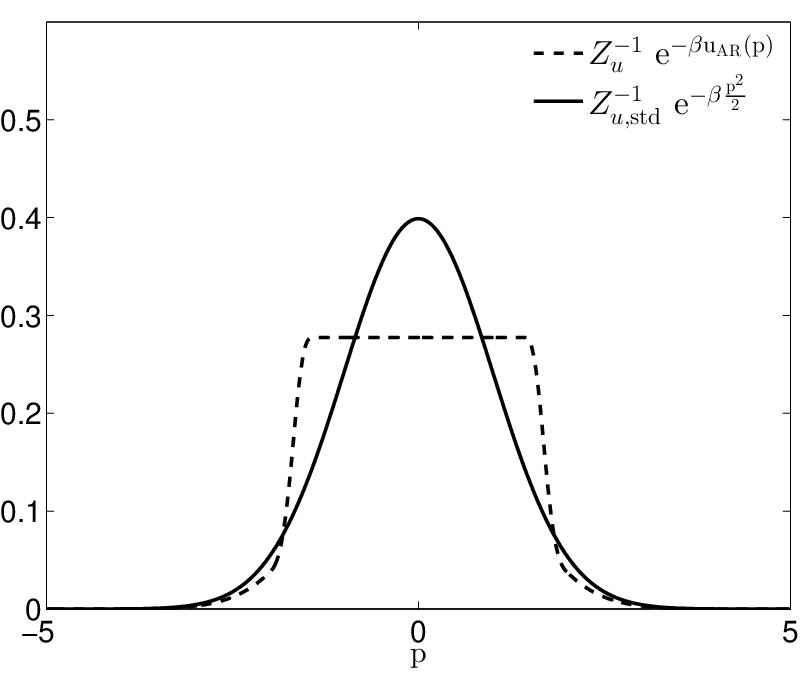
An appropriate function allows to smoothly interpolate between these two limiting regimes (see Definition 1 for the precise expression). A possible choice of an individual kinetic energy uu, as well as the associated canonical distribution of momenta Zu−1​e−β​u​(p)​d​pZ_{u}^{-1}\mathrm{e}^{-\beta u(p)}\,dp are depicted in Figure 1 and Figure 2 when D=1D=1.

Refer to caption
Figure 1: Standard quadratic kinetic energy function UstdU_{\rm{std}} (solid lines), and an example of an AR kinetic energy function uu with parameters Kmax=2K_{\mathrm{max}}=2 and Kmin=1K_{\mathrm{min}}=1 (dashed line).
Refer to caption
Figure 2: Marginal canonical densities associated with the kinetic energy functions of Figure 1.

The interest of AR-Langevin dynamics is that, when their individual kinetic energies are sufficiently small, particles do not move. When two particles are frozen in this way, their pairwise interactions need not be updated. This allows decreasing the computational complexity of the force computation, which is typically the most time-consuming part of a molecular dynamics solver. Note that this can be generalized to higher-order interactions (such as three-body interactions based on bending angles for instance).

Remark 1

Note that, due to the additive structure of the kinetic energy, the momenta pip_{i} are independent and identically distributed (i.i.d.) under the canonical measure. It is however possible to choose different parameters KminK_{\mathrm{min}} and KmaxK_{\mathrm{max}} for different particles, for example to focus calculations on a specific part of the particle system, in which case the momenta are still independent but not longer identically distributed. Such a situation is considered in the numerical example presented in Section 5.2.

3 Ergodicity of the modified Langevin dynamics

There are several notions of ergodicity for stochastic processes. We focus here on two of them: the convergence of ergodic averages over a single trajectory, and the convergence of the law of the process.

3.1 Convergence of ergodic averages

The convergence of ergodic averages over one trajectory is automatically ensured by the existence of an invariant probability measure and the irreducibility of the dynamics (see for instance Kliemann (1987); Meyn and Tweedie (1993) for early results on such convergences for possibly degenerate diffusions). Since, by construction, an invariant probability measure is known (namely the canonical measure (7)), it suffices to show that the process generated by the modified Langevin equation is irreducible to conclude to the convergence of ergodic averages.

As reviewed in Rey-Bellet (2006), the most standard argument to prove the irreducibility of degenerate diffusions is to prove the controllability of the dynamics relying on the Stroock-Varadhan support theorem, and the regularity of the transition kernel thanks to some hypoellipticity property. These conditions are satisfied for standard Langevin dynamics (see for instance Mattingly et al. (2002)), but not for the modified Langevin dynamics we consider, since the Hessian of the kinetic energy function may not be invertible on an open set. This is the case for the AR kinetic energy function presented in Section 2.1.

To illustrate this point, let us show for instance how the standard way of proving hypoellipticity fails (the proof of the controllability faces similar issues). The first task is to rewrite the generator (6) of the process as

ℒ=X0−∑j=1dXj†​Xj,\mathcal{L}=X_{0}-\sum_{j=1}^{d}X_{j}^{\dagger}X_{j},

where

X0=∇U⋅∇q−∇V⋅∇p−γ∇U⋅∇p,Xj=γβ∂pj,X_{0}=\nabla U\cdot\nabla_{q}-\nabla V\cdot\nabla_{p}-\gamma\nabla U\cdot\nabla_{p},\qquad X_{j}=\sqrt{\frac{\gamma}{\beta}}\,\partial_{p_{j}},

and Xj†X_{j}^{\dagger} is the adjoint of XjX_{j} on the flat space L2​(ℰ)L^{2}(\mathcal{E}). We next compute, for j=1,…,dj=1,\dots,d, the commutators

[X0,Xj]=X0Xj−XjX0=γβ∇(∂pjU)⋅(∇q−γ∇p).\displaystyle\left[X_{0},X_{j}\right]=X_{0}X_{j}-X_{j}X_{0}=\sqrt{\frac{\gamma}{\beta}}\,\nabla\left(\partial_{p_{j}}U\right)\cdot\left(\nabla_{q}-\gamma\nabla_{p}\right).

When ∇2U\nabla^{2}U is invertible, it is possible to recover the full algebra of derivatives by an appropriate combination of X1,…,XdX_{1},\dots,X_{d} and [X0,X1],…,[X0,Xd][X_{0},X_{1}],\dots,[X_{0},X_{d}]. Here, we consider a situation when this is not the case and, even more dramatically, where the Hessian may vanish on an open set. In this situation, [X0,Xj]=0\left[X_{0},X_{j}\right]=0 on the same open set, and in fact all iterated commutators [X0,[…​[X0,Xj]]][X_{0},[\dots[X_{0},X_{j}]]] also vanish.

We solve this problem by a direct constructive approach, where we see the modified dynamics as a perturbation of the standard Langevin dynamics. We rely on the following assumption:

Assumption 3.1

The kinetic energy function U∈C∞U\in C^{\infty} of the modified Langevin dynamics is such that

‖∇U−∇Ustd‖L∞⩽Gstd\left\|\nabla U-\nabla U_{\rm std}\right\|_{L^{\infty}}\leqslant G_{\mathrm{std}}

for some constant Gstd<+∞G_{\mathrm{std}}<+\infty.

Under this assumption, we can prove that the modified Langevin dynamics is irreducible by proving an appropriate minorization condition, which crucially relies on the compactness of the position space 𝒟\mathcal{D} (see Section 6.2 for the proof).

Lemma 1 (Minorization condition)

Suppose Assumption 3.1 holds. Then for any fixed p∗>0p^{*}>0 and t>0t>0, there exists a probability measure νp∗,t\nu_{p^{*},t} on 𝒟×ℝd\mathcal{D}\times\mathbb{R}^{d} and a constant κ>0\kappa>0 such that, for every Borel set B∈ℬ⁡(ℰ)B\in\mathscr{B}(\mathcal{E}),

ℙ⁡((qt,pt)∈B||p0|⩽p∗)⩾κ​νp∗,t​(B),\mathbb{P}\left((q_{t},p_{t})\in B\,\Big|\,\left|p_{0}\right|\leqslant p_{*}\right)\geqslant\kappa\,\nu_{p_{*},t}(B),

with νp∗,t​(B)>0\nu_{p_{*},t}(B)>0 when |B|>0\left|B\right|>0.

The minorization condition implies the irreducibility of the dynamics, so that the following convergence result readily follows.

Theorem 3.2 (Convergence of ergodic averages)

When Assumption 3.1 holds, ergodic averages over trajectories almost surely converge to the canonical average:

∀A∈L1(μ),limt→+∞1t∫0tA(qs,ps)ds=∫ℰAdμa.s.\forall A\in L^{1}(\mu),\qquad\lim_{t\rightarrow+\infty}\frac{1}{t}\int_{0}^{t}A(q_{s},p_{s})ds=\int_{\mathcal{E}}A\,d\mu\quad\mathrm{a.s.}

3.2 Convergence of the law

There are various functional frameworks to measure the convergence of the law of the process. We consider here weighted L∞L^{\infty} estimates on the semi-group et​ℒ\mathrm{e}^{t\mathcal{L}}. More precisely, we introduce a scale of Lyapunov functions

𝒦s​(p):=1+|p|2​s\mathcal{K}_{s}(p):=1+\left|p\right|^{2s} (8)

for s∈ℕ∗s\in\mathbb{N}^{*}. Recall indeed that only momenta need to be controlled since positions remain in a compact space. The associated weighted L∞L^{\infty} spaces are

L𝒦s∞={fmeasurable|‖f‖L𝒦s∞:=‖f𝒦s‖L∞<+∞}.L^{\infty}_{\mathcal{K}_{s}}=\left\{f\,\mathrm{measurable}\,\left|\,\left\|f\right\|_{L^{\infty}_{\mathcal{K}_{s}}}:=\left\|\frac{f}{\mathcal{K}_{s}}\right\|_{L^{\infty}}<+\infty\right.\right\}.

In order to prove the exponential convergence of the law, we rely on the result of Hairer and Mattingly (2011), which states that if a Lyapunov condition and a minorization condition hold true, then the sampled chain converges exponentially fast to its steady state in the following sense.

Theorem 3.3 (Exponential convergence of the law)

Suppose that Assumption 3.1 holds. Then the invariant measure μ\mu is unique, and for any s∈ℕ∗s\in\mathbb{N}^{*}, there exist constants Cs,λs>0C_{s},\lambda_{s}>0 such that

∀f∈L𝒦s∞,∀t⩾0,‖et​ℒ​f−∫ℰf​𝑑μ‖L𝒦s∞⩽Cs​e−λs​t​‖f‖L𝒦s∞.\forall f\in L^{\infty}_{\mathcal{K}_{s}},\quad\forall\ t\geqslant 0,\qquad\left\|\mathrm{e}^{t\mathcal{L}}f-\int_{\mathcal{E}}fd\mu\right\|_{L^{\infty}_{\mathcal{K}_{s}}}\leqslant C_{s}\mathrm{e}^{-\lambda_{s}t}\left\|f\right\|_{L^{\infty}_{\mathcal{K}_{s}}}. (9)

As mentioned above, the proof of this result directly follows from the arguments of Hairer and Mattingly (2011). The minorization condition is already stated in Lemma 1, while the appropriate Lyapunov condition reads as follows (see Section 6.1 for the proof, which uses the same strategy as Leimkuhler et al. (2015) and Joubaud et al. (2015)).

Lemma 2 (Lyapunov Condition)

Suppose that Assumption 3.1 holds. Then, for any s⩾1s\geqslant 1 and t>0t>0, there exist b>0b>0 and a∈[0,1)a\in\left[0,1\right) such that

et​ℒ​𝒦s⩽a​𝒦s+b.\mathrm{e}^{t\mathcal{L}}\mathcal{K}_{s}\leqslant a\mathcal{K}_{s}+b.

3.3 Regularity results for the evolution semi-group

We provide in this section decay estimates for the spatial derivatives of et​ℒ​f\mathrm{e}^{t\mathcal{L}}f, following the approach pioneered in Talay (2002) and further refined in Kopec (2013). Such estimates were obtained for the standard Langevin dynamics, but can in fact straightforwardly be extended to modified Langevin dynamics with Hessians bounded from below by a positive constant. Our aim in this section is to provide decay estimates for the spatial derivatives of et​ℒ​f\mathrm{e}^{t\mathcal{L}}f in the situation when ∇2U\nabla^{2}U fails to be strictly convex, for instance because ∇2U\nabla^{2}U vanishes on an open set as is the case for AR particle simulations.

In order to state our results, we first need to define the weighted Sobolev spaces 𝒲𝒦sn,∞\mathscr{W}^{n,\infty}_{\mathcal{K}_{s}} for n∈ℕn\in\mathbb{N}:

𝒲𝒦sn,∞={f∈L𝒦s∞|∀k∈ℕ2​d,|k|⩽n,∂kf∈L𝒦s∞}.\displaystyle\mathscr{W}^{n,\infty}_{\mathcal{K}_{s}}=\Big\{f\in L^{\infty}_{\mathcal{K}_{s}}\left|\ \forall k\in\mathbb{N}^{2d},\ \left|k\right|\leqslant n,\ \partial^{k}f\in L^{\infty}_{\mathcal{K}_{s}}\Big\}\right..

These spaces gather all functions which grow at most like 𝒦s\mathcal{K}_{s}, and whose derivatives of order at most nn all grow at most like 𝒦s\mathcal{K}_{s}. We also introduce the space of smooth functions 𝒮\mathscr{S}, the vector space of functions f∈L2​(μ)\displaystyle f\in L^{2}\left(\mu\right) such that, for any n⩾0n\geqslant 0, there exists r∈ℕr\in\mathbb{N} for which f∈𝒲𝒦rn,∞f\in\mathscr{W}^{n,\infty}_{\mathcal{K}_{r}}.

We also make the following assumption on the kinetic energy function, which can be understood as a condition of “almost strict convexity” of the Hessian ∇2U\nabla^{2}U.

Assumption 3.4

The kinetic energy U∈𝒮U\in\mathscr{S} has bounded second-order derivatives:

sup|j|=2‖∂jU‖L∞<∞,\sup_{\left|j\right|=2}\left\|\partial^{j}U\right\|_{L^{\infty}}<\infty\,, (10)

and there exist a function Uν∈𝒮U_{\nu}\in\mathscr{S} and constants ν>0\nu>0 and Gν⩾0G_{\nu}\geqslant 0 such that

∇2Uν⩾ν>0\nabla^{2}U_{\nu}\geqslant\nu>0 (11)

and

‖∇(U−Uν)‖L∞⩽Gν.\left\|\nabla\left(U-U_{\nu}\right)\right\|_{L^{\infty}}\leqslant G_{\nu}. (12)
Remark 2

A natural choice for the function UνU_{\nu} in Assumption 3.4 is UstdU_{\rm{std}}. The condition (11) then holds with ν=1/max⁡(m1,…,mN)\nu=1/\max(m_{1},\dots,m_{N}). Moreover, (10) holds true as soon as UU is a local perturbation of UstdU_{\rm std}. The most demanding condition therefore is (12), especially if GνG_{\nu} has to be small.

By following the same strategy as in (Kopec, 2013, Proposition A.1.) (which refines the results already obtained in Talay (2002)), and appropriately taking care of the lack of strict positivity of the Hessian ∇2U\nabla^{2}U by assuming that GνG_{\nu} is sufficiently small, we prove the following result in Section 6.3.

Lemma 3

Suppose that Assumptions 3.1 and 3.4 hold, and fix A∈𝒮A\in\mathscr{S}. For any n⩾1n\geqslant 1, there exist n~,sn∈ℕ\widetilde{n},s_{n}\in\mathbb{N} and λn>0\lambda_{n}>0 such that, for s⩾sns\geqslant s_{n} and Gν⩽ρs\displaystyle G_{\nu}\leqslant\rho_{s} with ρs>0\rho_{s}>0 sufficiently small (depending on ss but not on nn), there is r∈ℕr\in\mathbb{N} and C>0C>0 for which

∀t⩾0,∀|k|⩽n,‖∂ket​ℒ​Πμ​A‖L𝒦s∞⩽C​‖A‖W𝒦rn~,∞​e−λn​t.\forall t\geqslant 0,\quad\forall\left|k\right|\leqslant n,\qquad\left\|\partial^{k}\mathrm{e}^{t\mathcal{L}}\Pi_{\mu}A\right\|_{L^{\infty}_{\mathcal{K}_{s}}}\leqslant C\left\|A\right\|_{W^{\widetilde{n},\infty}_{\mathcal{K}_{r}}}\mathrm{e}^{-\lambda_{n}t}. (13)

The parameter ρs\rho_{s} can in fact be made explicit, see (36) below. The decay estimate (13) shows that the derivatives of the evolution operator can be controlled in appropriate weighted Hilbert spaces. Note however that the Lyapunov functions entering in the estimates are not the same a priori on both sides of the inequality (13). Let us emphasize, though, that we can obtain a control in all spaces L𝒦s∞L^{\infty}_{\mathcal{K}_{s}} for ss sufficiently large (depending on the order of derivation).

4 Analysis of the statistical error

The asymptotic variance characterizes the statistical error. In Section 4.1, we show that the asymptotic variance is well defined for the modified Langevin dynamics. We can in fact prove a stronger result, namely that a Central Limit Theorem (CLT) holds true for ergodic averages over one trajectory. In a second step, we more carefully analyze in Section 4.2 the properties of the variance of the AR-Langevin dynamics by proving a linear response result in the limit of a vanishing lower bound on the kinetic energies. To obtain the latter results, we rely on the estimates provided by Lemma 3.

4.1 A Central Limit theorem for ergodic averages

Let us first write the asymptotic variance in terms of the generator of the dynamics. To simplify the notation, we introduce the orthogonal projection Πμ\Pi_{\mu} onto the orthogonal of the kernel of the operator ℒ\mathcal{L} (with respect to the L2​(μ)L^{2}(\mu) scalar product): for any ψ∈L2​(μ)\psi\in L^{2}(\mu),

Πμ​ψ:=ψ−∫ℰψ​𝑑μ.\Pi_{\mu}\psi:=\psi-\int_{\mathcal{E}}\psi\,d\mu.

Since L𝒦s∞⊂L2​(μ)L^{\infty}_{\mathcal{K}_{s}}\subset L^{2}(\mu), we can define L𝒦s∞~=Πμ​(L𝒦s∞)\displaystyle\widetilde{L^{\infty}_{\mathcal{K}_{s}}}=\Pi_{\mu}\left(L^{\infty}_{\mathcal{K}_{s}}\right). The ergodicity result (9) allows us to conclude that the operator ℒ\mathcal{L} is invertible on L𝒦s∞~\widetilde{L^{\infty}_{\mathcal{K}_{s}}} since the following operator equality holds on ℬ⁡(L𝒦s∞~)\mathcal{B}\left(\widetilde{L^{\infty}_{\mathcal{K}_{s}}}\right), the Banach space of bounded operators on L𝒦s∞~\widetilde{L^{\infty}_{\mathcal{K}_{s}}}:

ℒ−1=∫0+∞et​ℒ​𝑑t.\mathcal{L}^{-1}=\int_{0}^{+\infty}\mathrm{e}^{t\mathcal{L}}\,dt.

This leads to the following resolvent bounds (the second part being a direct corollary of Lemma 3).

Corollary 1

Suppose that Assumption 3.1 holds. Then, for any s∈ℕ∗s\in\mathbb{N}^{*},

‖ℒ−1‖ℬ⁡(L𝒦s∞~)⩽Csλs,\left\|\mathcal{L}^{-1}\right\|_{\mathcal{B}\left(\widetilde{L^{\infty}_{\mathcal{K}_{s}}}\right)}\leqslant\frac{C_{s}}{\lambda_{s}}, (14)

where λs,Cs\lambda_{s},C_{s} are the constants introduced in Theorem 3.3. Suppose in addition that Assumption 3.4 holds, and fix A∈𝒮A\in\mathscr{S}. For any n⩾1n\geqslant 1, there exist n~,sn∈ℕ\widetilde{n},s_{n}\in\mathbb{N} and λn>0\lambda_{n}>0 such that, for s⩾sns\geqslant s_{n} and Gν⩽ρs\displaystyle G_{\nu}\leqslant\rho_{s} with ρs>0\rho_{s}>0 sufficiently small (depending on ss but not on nn), there is r∈ℕr\in\mathbb{N} and C>0C>0 for which

∀|k|⩽n,‖∂kℒ−1​Πμ​A‖L𝒦s∞⩽Cλn​‖A‖W𝒦rn~,∞.\forall\left|k\right|\leqslant n,\qquad\left\|\partial^{k}\mathcal{L}^{-1}\Pi_{\mu}A\right\|_{L^{\infty}_{\mathcal{K}_{s}}}\leqslant\frac{C}{\lambda_{n}}\left\|A\right\|_{W^{\widetilde{n},\infty}_{\mathcal{K}_{r}}}. (15)

This already allows us to conclude that the asymptotic variance of the time average A^t\widehat{A}_{t} defined in (1) is well defined for any observable A∈L𝒦r∞A\in L^{\infty}_{\mathcal{K}_{r}} since

σA2\displaystyle\sigma_{A}^{2} =limt→∞t​𝔼​[(A^t−𝔼μ​(A))2]\displaystyle=\lim_{t\rightarrow\infty}t\,\mathbb{E}\Big[\left(\hat{A}_{t}-\mathbb{E}_{\mu}\left(A\right)\right)^{2}\Big]
=limt→∞2​∫0t∫ℰ(1−st)​(es​ℒ​Πμ​A)​(Πμ​A)​𝑑μ\displaystyle=\lim_{t\rightarrow\infty}2\int_{0}^{t}\int_{\mathcal{E}}\left(1-\frac{s}{t}\right)\left(\rm{e}^{s\mathcal{L}}\Pi_{\mu}A\right)\left(\Pi_{\mu}A\right)d\mu
=2​∫0∞∫ℰ(es​ℒ​Πμ​A)​(Πμ​A)​𝑑μ\displaystyle=2\int_{0}^{\infty}\int_{\mathcal{E}}\left(\mathrm{e}^{s\mathcal{L}}\Pi_{\mu}A\right)\left(\Pi_{\mu}A\right)d\mu

by the dominated convergence theorem. Therefore,

σA2=2​∫ℰ(Πμ​A)​(−ℒ−1​Πμ​A)​𝑑μ.\sigma^{2}_{A}=2\int_{\mathcal{E}}\left(\Pi_{\mu}A\right)\left(-\mathcal{L}^{-1}\Pi_{\mu}A\right)\,d\mu. (16)

In fact, a Central Limit Theorem can be shown to hold for A^t\widehat{A}_{t} using standard results (see e.g. Bhattacharya (1982)).

4.2 Perturbative study of the variance for the AR-Langevin dynamics

Our aim in this section is to better understand, from a quantitative viewpoint, the behavior of the asymptotic variance for the AR-Langevin dynamics defined in Section 2.1, at least in some limiting regime where the parameter KminK_{\mathrm{min}} is small. For intermediate values, we need to rely on numerical simulations (see Section 5).

The regime where both KminK_{\mathrm{min}} and KmaxK_{\mathrm{max}} go to 0 is somewhat singular since the transition from U⁡(p)=0U(p)=0 to U​(p)=Ustd​(p)U(p)=U_{\rm std}(p) becomes quite abrupt, which prevents a rigorous theoretical analysis. The regimes where either KminK_{\mathrm{min}} or KmaxK_{\mathrm{max}} go to infinity are also of dubious interest since the dynamics strongly perturbs the standard Langevin dynamics. Therefore, we restrict ourselves to the situation where Kmin→0K_{\mathrm{min}}\to 0 with KmaxK_{\mathrm{max}} fixed.

In order to highlight the dependence of the AR kinetic energy function on the restraining parameters 0⩽Kmin<Kmax0\leqslant K_{\mathrm{min}}<K_{\mathrm{max}}, we denote it by UKmin,KmaxU_{K_{\mathrm{min}},K_{\mathrm{max}}} in the remainder of this section. Let us however first give a more precise definition of this function, having in mind that KmaxK_{\mathrm{max}} is fixed while KminK_{\mathrm{min}} eventually goes to 0. We introduce to this end an interpolation function f0,Kmax∈C∞​(ℝ)f_{0,K_{\mathrm{max}}}\in C^{\infty}\left(\mathbb{R}\right) such that

0⩽f0,Kmax⩽1,f0,Kmax​(x)=1​for​x⩽0,f0,Kmax​(x)=0​for​x⩾Kmax,0\leqslant f_{0,K_{\mathrm{max}}}\leqslant 1,\qquad f_{0,K_{\mathrm{max}}}(x)=1\ \mathrm{for}\ x\leqslant 0,\qquad f_{0,K_{\mathrm{max}}}(x)=0\ \mathrm{for}\ x\geqslant K_{\mathrm{max}}, (17)

and

∀n⩾1,f0,Kmax(n)​(0)=f0,Kmax(n)​(Kmax)=0.\forall n\geqslant 1,\qquad f_{0,K_{\mathrm{max}}}^{(n)}(0)=f_{0,K_{\mathrm{max}}}^{(n)}(K_{\mathrm{max}})=0.

We next define an interpolation function fKmin,Kmaxf_{K_{\mathrm{min}},K_{\mathrm{max}}} obtained from the function f0,Kmaxf_{0,K_{\mathrm{max}}} by an appropriate shift of the lower bound and a rescaling. More precisely, fKmin,Kmax​(x)=f0,Kmax​(θKmin​(x))f_{K_{\mathrm{min}},K_{\mathrm{max}}}(x)=f_{0,K_{\mathrm{max}}}(\theta_{K_{\mathrm{min}}}(x)) with

θKmin(x):={x−Kmin,for ​x⩽Kmin,KmaxKmax−Kmin​(x−Kmin),for ​Kmin⩽x⩽Kmax,x,for ​x⩾Kmax.\theta_{K_{\mathrm{min}}}(x):=\left\{\displaystyle\begin{aligned} x-K_{\mathrm{min}},&\quad\text{for }x\leqslant K_{\mathrm{min}},\\ \frac{K_{\mathrm{max}}}{K_{\mathrm{max}}-K_{\mathrm{min}}}(x-K_{\mathrm{min}}),&\quad\text{for }K_{\mathrm{min}}\leqslant x\leqslant K_{\mathrm{max}},\\ x,&\quad\text{for }x\geqslant K_{\mathrm{max}}.\end{aligned}\right. (18)

A plot of fKmin,Kmaxf_{K_{\mathrm{min}},K_{\mathrm{max}}} is provided in Figure 3.

Refer to caption
Figure 3: Functions f0,Kmaxf_{0,K_{\mathrm{max}}} and fKmin,Kmaxf_{K_{\mathrm{min}},K_{\mathrm{max}}} for Kmax=2K_{\mathrm{max}}=2 and Kmin=1K_{\mathrm{min}}=1.
Refer to caption
Figure 4: Standard kinetic energy function UstdU_{\rm{std}}, as well as two AR kinetic energy functions UKmin,KmaxU_{K_{\mathrm{min}},K_{\mathrm{max}}} with Kmax=2K_{\mathrm{max}}=2 and Kmin=0K_{\mathrm{min}}=0 or 11.
Definition 1 (AR kinetic energy function)

For two parameters 0⩽Kmin<Kmax0\leqslant K_{\mathrm{min}}<K_{\mathrm{max}}, the AR kinetic energy function UKmin,KmaxU_{K_{\mathrm{min}},K_{\mathrm{max}}} is defined as

UKmin,Kmax​(p):=∑i=1NuKmin,Kmax​(pi),U_{K_{\mathrm{min}},K_{\mathrm{max}}}(p):=\sum_{i=1}^{N}u_{K_{\mathrm{min}},K_{\mathrm{max}}}(p_{i}), (19)

where the individual kinetic energy functions are

uKmin,Kmax(pi):={0,for ​pi22​mi⩽Kmin,[1−fKmin,Kmax​(pi22​mi)]​pi22​mi,for ​pi22​mi∈[Kmin,Kmax],pi22​mi,for ​pi22​mi⩾Kmax.u_{K_{\mathrm{min}},K_{\mathrm{max}}}(p_{i}):=\left\{\begin{aligned} \displaystyle 0,&\quad\text{for }\frac{p_{i}^{2}}{2m_{i}}\leqslant K_{\mathrm{min}},\\ \left[1-f_{K_{\mathrm{min}},K_{\mathrm{max}}}\left(\frac{p_{i}^{2}}{2m_{i}}\right)\right]\frac{p_{i}^{2}}{2m_{i}},&\quad\text{for }\frac{p_{i}^{2}}{2m_{i}}\in[K_{\mathrm{min}},K_{\mathrm{max}}],\\ \frac{p_{i}^{2}}{2m_{i}},&\quad\text{for }\frac{p_{i}^{2}}{2m_{i}}\geqslant K_{\mathrm{max}}.\\ \end{aligned}\right. (20)

Of course, UKmin,Kmax​(p)U_{K_{\mathrm{min}},K_{\mathrm{max}}}(p) converges to U0,Kmax​(p)U_{0,K_{\mathrm{max}}}(p) as Kmin→0K_{\mathrm{min}}\to 0. The limiting kinetic energy function U0,KmaxU_{0,K_{\mathrm{max}}} corresponds to what we call the Zero-KmaxK_{\mathrm{max}}-AR-Langevin dynamics (see Figure 4 for an illustration). Let us emphasize that the limiting dynamics is not the standard Langevin dynamics, so that the expansion in powers of KminK_{\mathrm{min}} of the variance we provide is with respect to the limiting variance of the dynamics corresponding to U0,KmaxU_{0,K_{\mathrm{max}}}. To simplify the notation, we denote by σ2​(Kmin)\sigma^{2}(K_{\mathrm{min}}) the variance associated with the kinetic energy UKmin,KmaxU_{K_{\mathrm{min}},K_{\mathrm{max}}}.

Proposition 1

There exists Kmax∗>0K_{\mathrm{max}}^{*}>0 such that, for any 0<Kmax⩽Kmax∗0<K_{\mathrm{max}}\leqslant K_{\mathrm{max}}^{*}, there is a constant 𝒦>0\mathscr{K}>0 for which

∀0⩽Kmin⩽Kmax2,σA2​(Kmin)=σA2​(0)+𝒦​Kmin+O⁡(Kmin2).\forall 0\leqslant K_{\mathrm{min}}\leqslant\frac{K_{\mathrm{max}}}{2},\qquad\sigma_{A}^{2}(K_{\mathrm{min}})=\sigma_{A}^{2}(0)+\mathscr{K}K_{\mathrm{min}}+\mathrm{O}(K_{\mathrm{min}}^{2}). (21)

The proof can be read in Section 6.4. The assumption that KmaxK_{\mathrm{max}} is sufficiently small ensures that Assumption 3.4 holds (see Section 6.4.3). The result is formally clear. The difficulty in proving it is that the kinetic energy is not a smooth function of KminK_{\mathrm{min}} because the shift function is only piecewise smooth.

Remark 3

An inspection of the proof of Proposition 1 shows that the linear response result can be generalized to non-zero values of KminK_{\mathrm{min}} and in fact to linear responses in the parameter KmaxK_{\mathrm{max}} as well. For the latter case, we consider f0,Kmax​(x)=f0,1​(x/Kmax)f_{0,K_{\mathrm{max}}}(x)=f_{0,1}(x/K_{\mathrm{max}}). Denoting now by σ2​(Kmin,Kmax)\sigma^{2}(K_{\mathrm{min}},K_{\mathrm{max}}) the variance associated with the kinetic energy UKmin,KmaxU_{K_{\mathrm{min}},K_{\mathrm{max}}}, it can be proved that, for 0<Kmin<Kmax0<K_{\mathrm{min}}<K_{\mathrm{max}} not too large, there are a,b∈ℝa,b\in\mathbb{R} such that, for δ,η∈ℝ\delta,\eta\in\mathbb{R} sufficiently small,

σ2​(Kmin+δ,Kmax+η)=σ2​(Kmin,Kmax)+a​δ+b​η+O⁡(η2+δ2).\sigma^{2}(K_{\mathrm{min}}+\delta,K_{\mathrm{max}}+\eta)=\sigma^{2}(K_{\mathrm{min}},K_{\mathrm{max}})+a\delta+b\eta+\mathrm{O}(\eta^{2}+\delta^{2}).

5 Numerical results

The aim of this section is to quantify the evolution of the variance of AR-Langevin dynamics as the parameters of the kinetic energy function are modified. We first consider in Section 5.1 a simple system in spatial dimension 1, for which the variance can be very precisely computed using a Galerkin-type approximation. We next consider more realistic particle systems in Section 5.2, relying on molecular dynamics simulations to estimate the variance. In this section, the function f0,Kmax​(x)f_{0,K_{\mathrm{max}}}(x) is chosen to be of the form f0,1​(x/Kmax)f_{0,1}(x/K_{\mathrm{max}}), with f0,1f_{0,1} a fifth-order spline function.

5.1 A simple one-dimensional system

We first consider a single particle in spatial dimension d=1d=1, in the periodic domain 𝒟=2​π​𝕋\mathcal{D}=2\pi\mathbb{T} and at inverse temperature β=1\beta=1. In this case, it is possible to directly approximate the asymptotic variance (16) using some Galerkin discretization, as in Risken (1984) or Latorre et al. (2013).

We denote by ℒKmin,Kmax\mathcal{L}_{K_{\mathrm{min}},K_{\mathrm{max}}} the generator of the modified Langevin dynamics associated with the AR kinetic energy function UKmin,KmaxU_{K_{\mathrm{min}},K_{\mathrm{max}}} defined in (19), by μKmin,Kmax\mu_{K_{\mathrm{min}},K_{\mathrm{max}}} the associated canonical measure, and by ΠKmin,Kmax\Pi_{K_{\mathrm{min}},K_{\mathrm{max}}} the projector onto functions of L2​(μKmin,Kmax)L^{2}(\mu_{K_{\mathrm{min}},K_{\mathrm{max}}}) with average 0 with respect to μKmin,Kmax\mu_{K_{\mathrm{min}},K_{\mathrm{max}}}.

For a given observable AA, we first approximate the solution of the following Poisson equation:

−ℒKmin,Kmax​ΦA=ΠKmin,Kmax​A,-\mathcal{L}_{K_{\mathrm{min}},K_{\mathrm{max}}}\Phi_{A}=\Pi_{K_{\mathrm{min}},K_{\mathrm{max}}}A, (22)

and then compute the variance as given by (16):

σA2=2​∫ℰΦA​A​d​μKmin,Kmax.\sigma_{A}^{2}=2\int_{\mathcal{E}}\Phi_{A}\,A\,d\mu_{K_{\mathrm{min}},K_{\mathrm{max}}}.

To achieve this, we introduce the basis functions ψn​k​(q,p):=Gk​(q)​Hn​(p)\psi_{nk}(q,p):=G_{k}(q)\,H_{n}(p), where Gk(q)=(2π)−1/2ei​k​qG_{k}(q)=(2\pi)^{-1/2}\mathrm{e}^{\mathrm{i}kq} (for k∈ℤk\in\mathbb{Z}) and Hn​(p)H_{n}(p) are the Hermite polynomials:

Hn(p)=(−1)nep2/2dnd​pn(e−p2/2),∀n∈ℕ.\qquad H_{n}(p)=(-1)^{n}\mathrm{e}^{p^{2}/2}\frac{d^{n}}{dp^{n}}\Big(\mathrm{e}^{-p^{2}/2}\Big),\forall n\in\mathbb{N}.

The choice of GkG_{k} is natural in view of the spatial periodicity of the functions under consideration, while Hermite polynomials are eigenfunctions of the generator associated with the Ornstein-Uhlenbeck process on the momenta for the standard quadratic kinetic energy p2/2p^{2}/2. Note however that, when the kinetic energy is modified as UKmin,KmaxU_{K_{\mathrm{min}},K_{\mathrm{max}}}, the Hermite polynomials are no longer orthogonal for the L2​(μKmin,Kmax)L^{2}(\mu_{K_{\mathrm{min}},K_{\mathrm{max}}}) scalar product.

We approximate the Poisson equation (22) on the basis
𝒱NG,NH={ψn​k}0⩽n⩽NH,−NG⩽k⩽NG\mathcal{V}_{N_{G},N_{H}}=\{\psi_{nk}\}_{0\leqslant n\leqslant N_{H},\,-N_{G}\leqslant k\leqslant N_{G}} for given integers NG,HH⩾1N_{G},H_{H}\geqslant 1, and we look for approximate solutions of the form ΠKmin,Kmax​ΦANG,NH\Pi_{K_{\mathrm{min}},K_{\mathrm{max}}}\Phi_{A}^{N_{G},N_{H}} with

ΦANG,NH=∑n=−NHNH∑k=0NG[bNG,NH]n​k​ψn​k,\Phi_{A}^{N_{G},N_{H}}=\sum_{n=-N_{H}}^{N_{H}}\sum_{k=0}^{N_{G}}\left[b_{N_{G},N_{H}}\right]_{nk}\psi_{nk},

where bNG,NH=(bn​k)0⩽n⩽NH,−NG⩽k⩽NGb_{N_{G},N_{H}}=(b_{nk})_{0\leqslant n\leqslant N_{H},\,-N_{G}\leqslant k\leqslant N_{G}} is a vector of size (2​NG+1)​(NH+1)(2N_{G}+1)(N_{H}+1). Restricting (22) to 𝒱NG,NH\mathcal{V}_{N_{G},N_{H}} leads to

MNG,NH​bNG,NH=aNG,NH,M_{N_{G},N_{H}}b_{N_{G},N_{H}}=a_{N_{G},N_{H}}, (23)

where MNG,NHM_{N_{G},N_{H}} is a matrix of size (2​NG+1)​(NH+1)×(2​NG+1)​(NH+1)(2N_{G}+1)(N_{H}+1)\times(2N_{G}+1)(N_{H}+1) and aNG,NHa_{N_{G},N_{H}} a vector of size (2​NG+1)​(NH+1)(2N_{G}+1)(N_{H}+1), whose entries respectively read

[MNG,NH]n​k,m​l\displaystyle\left[M_{N_{G},N_{H}}\right]_{nk,ml} =⟨ψm​l,−ℒKmin,Kmax​ψn​k⟩L2​(μKmin,Kmax),\displaystyle=\left\langle\psi_{ml},-\mathcal{L}_{K_{\mathrm{min}},K_{\mathrm{max}}}\psi_{nk}\right\rangle_{L^{2}(\mu_{K_{\mathrm{min}},K_{\mathrm{max}}})},
[aNG,NH]m​l\displaystyle\left[a_{N_{G},N_{H}}\right]_{ml} =⟨ψm​l,ΠKmin,Kmax​A⟩L2​(μKmin,Kmax).\displaystyle=\left\langle\psi_{ml},\Pi_{K_{\mathrm{min}},K_{\mathrm{max}}}A\right\rangle_{L^{2}(\mu_{K_{\mathrm{min}},K_{\mathrm{max}}})}.

The approximated solution ΦANG,NH\Phi_{A}^{N_{G},N_{H}} of the Poisson equation (22) can therefore be computed by solving (23). Note however that some care is needed at this stage since ℒKmin,Kmax\mathcal{L}_{K_{\mathrm{min}},K_{\mathrm{max}}} is not invertible on 𝒱NG,NH\mathcal{V}_{N_{G},N_{H}}, because the basis functions {ψn​k}0⩽n⩽NH,−NG⩽k⩽NG\{\psi_{nk}\}_{0\leqslant n\leqslant N_{H},\,-N_{G}\leqslant k\leqslant N_{G}} are not of integral 0 with respect to μKmin,Kmax\mu_{K_{\mathrm{min}},K_{\mathrm{max}}}. We correct this by performing a singular value decomposition of MNG,NHM_{N_{G},N_{H}}, removing the component of aNG,NHa_{N_{G},N_{H}} associated with the singular value 0, and computing the inverse of MNG,NHM_{N_{G},N_{H}} on the subspace generated by the eigenvectors associated with non-zero eigenvalues. In practice, we compute the entries of aNG,NHa_{N_{G},N_{H}} and MNG,NHM_{N_{G},N_{H}} by numerical quadrature. Since the Hermite polynomials are no longer orthogonal for the L2​(μKmin,Kmax)L^{2}(\mu_{K_{\mathrm{min}},K_{\mathrm{max}}}) scalar product, quadratures are required both in position and momentum variables. The variance is finally approximated as

σA2​(NG,NH)=2​∫ℰA​ΦANG,NH​d​μKmin,Kmax=2​bNG,NHT​aNG,NH.\sigma_{A}^{2}(N_{G},N_{H})=2\int_{\mathcal{E}}A\,\Phi_{A}^{N_{G},N_{H}}\,d\mu_{K_{\mathrm{min}},K_{\mathrm{max}}}=2b_{N_{G},N_{H}}^{T}a_{N_{G},N_{H}}.

In the simulations presented in this section, the potential is V⁡(q)=cos⁡(q)V(q)=\cos(q), the observable under study is A=VA=V, and we always set NH=2​NG−1N_{H}=2N_{G}-1. Figure 5 presents the convergence of the variance with respect to the basis size, for the standard Langevin dynamics and the AR Langevin dynamics with Kmax=2K_{\mathrm{max}}=2 and various values of KminK_{\mathrm{min}}. The results show that the choice NG=12N_{G}=12 is sufficient in all cases to approximate the asymptotic value. We checked in addition in one case, namely for the standard dynamics, that the values we obtain are very close to a reference value obtained with NG=30N_{G}=30: the relative variation is of order 10−810^{-8} for NG=10N_{G}=10, 10−1010^{-10} for NG=12N_{G}=12 and 10−1110^{-11} for NG=14N_{G}=14. We therefore set NG=12N_{G}=12 in the remainder of this section.

Refer to caption
Figure 5: Convergence of the Galerkin approximation in the basis size NGN_{G} and NH=2​NG−1N_{H}=2N_{G}-1: approximation of the variance of observable A=VA=V for the standard dynamics and the AR dynamics with fixed parameter Kmax=2K_{\mathrm{max}}=2 and various values of KminK_{\mathrm{min}}.

The variation of the computed variance for A=VA=V is plotted in Figure 6 for various parameters 0⩽Kmin<Kmax0\leqslant K_{\mathrm{min}}<K_{\mathrm{max}} of the AR-Langevin dynamics. Note that, as expected, the variance increases with increasing values of KminK_{\mathrm{min}} for fixed KmaxK_{\mathrm{max}}, but also with increasing values of KmaxK_{\mathrm{max}} for fixed KminK_{\mathrm{min}}. We next illustrate the linear response results of Proposition 1 and Remark 3 in Figures 7 and  8: in both situations, the variance increases linearly with the parameter under consideration is varied in a sufficiently small neighborhood of its initial value. After that initial regime, nonlinear variations appear. Note also that the relative increase of the variance is more pronounced as a function of KmaxK_{\mathrm{max}} than KminK_{\mathrm{min}}.

Refer to caption
Figure 6: Asymptotic variance of time averages for A=VA=V, approximated by the Galerkin method, as a function of KminK_{\mathrm{min}} and for several values of KmaxK_{\mathrm{max}}.
Refer to caption
Figure 7: Relative difference between the variance σNG,NH2​(Kmin,Kmax)\sigma^{2}_{N_{G},N_{H}}(K_{\mathrm{min}},K_{\mathrm{max}}) and its initial value computed for reference parameters. (Left) Fixed upper bound Kmax=4K_{\mathrm{max}}=4, and reference value Kmin=0K_{\mathrm{min}}=0.
Refer to caption
Figure 8: Same as Figure 7. Fixed lower bound Kmin=0K_{\mathrm{min}}=0, and reference value Kmax=2K_{\mathrm{max}}=2.
Remark 4

In practice, the idea usually is to set the lower bound KminK_{\mathrm{min}} sufficiently large when performing Monte Carlo simulations, in order to decrease as much as possible the computational cost. The gap Kmax−KminK_{\mathrm{max}}-K_{\mathrm{min}} should however not be too small in order to have a sufficiently smooth transition from a vanishing kinetic energy to a quadratic one. This requires therefore KmaxK_{\mathrm{max}} to be quite large if KminK_{\mathrm{min}} is large. The results presented in Figure 8 suggest that this may not be the optimal choice, unless the algorithmic speed-up is quite large.

5.2 A more realistic system

In order to study the variation of the variance as a function of KminK_{\mathrm{min}} and KmaxK_{\mathrm{max}} in systems of higher dimensions, we resort to Monte Carlo simulations. This requires discretizing the AR-Langevin dynamics (5), and we resort to a scheme of weak order 2, obtained by a splitting strategy where the generator of the modified Langevin dynamics (6) is decomposed into three parts:

A:=∇U(p)⋅∇q,B:=−∇V(q)⋅∇p,C:=−∇U(p)⋅∇p+1βΔp.A:=\nabla U(p)\cdot\nabla_{q},\qquad B:=-\nabla V(q)\cdot\nabla_{p},\qquad C:=-\nabla U(p)\cdot\nabla_{p}+\frac{1}{\beta}\Delta_{p}\,.

The transition kernel obtained by a Strang splitting reads PΔ​t=eγ​Δ​t​C/2​eΔ​t​B/2​eΔ​t​A​eΔ​t​B/2​eγ​Δ​t​C/2P_{\Delta t}=\mathrm{e}^{\gamma\Delta tC/2}\mathrm{e}^{\Delta tB/2}\mathrm{e}^{\Delta tA}\mathrm{e}^{\Delta tB/2}\mathrm{e}^{\gamma\Delta tC/2}. Contrarily to the standard kinetic energy functions, the elementary evolution associated with CC cannot be integrated analytically. To preserve the order of the scheme, we approximate eγ​Δ​t/2​C\mathrm{e}^{\gamma\Delta t/2C} by a midpoint rule, encoded by a transition kernel PΔ​tγ,CP_{\Delta t}^{\gamma,C} satisfying PΔ​tγ,C​φ=eγ​Δ​t​C​φ+O⁡(Δ​t3)P_{\Delta t}^{\gamma,C}\varphi=\mathrm{e}^{\gamma\Delta tC}\varphi+\mathrm{O}(\Delta t^{3}) for smooth test functions φ\varphi. This gives the following discretization scheme:

{pn+1/4=pn−γ∇U(pn+1/4+pn2)Δ​t2+γ​Δ​tβGn,pn+1/2=pn+1/4−∇V​(qn)​Δ​t2,qn+1=qn+∇U​(pn+1/2)​Δ​t,pn+3/4=pn+1/2−∇V​(qn+1)​Δ​t2,pn+1=pn+3/4−γ∇U(pn+1+pn+3/42)Δ​t2+γ​Δ​tβGn+1/2,\displaystyle\left\{\begin{aligned} \displaystyle p^{n+1/4}&=p^{n}-\gamma\nabla U\left(\frac{p^{n+1/4}+p^{n}}{2}\right)\frac{\Delta t}{2}+\sqrt{\frac{\gamma\Delta t}{\beta}}G^{n},\\ p^{n+1/2}&=p^{n+1/4}-\nabla V(q^{n})\frac{\Delta t}{2},\\ q^{n+1}&=q^{n}+\nabla U(p^{n+1/2})\Delta t,\\ p^{n+3/4}&=p^{n+1/2}-\nabla V(q^{n+1})\frac{\Delta t}{2},\\ \displaystyle p^{n+1}&=p^{n+3/4}-\gamma\nabla U\left(\frac{p^{n+1}+p^{n+3/4}}{2}\right)\frac{\Delta t}{2}+\sqrt{\frac{\gamma\Delta t}{\beta}}G^{n+1/2},\end{aligned}\right.

where Gn,Gn+1/2G^{n},G^{n+1/2} are i.i.d. standard dd-dimensional Gaussian random variables. The first and the last line are obtained by implicit schemes, solved in practice by a fixed point strategy (the termination criterion being that the distance between successive iterates is smaller than 10−1010^{-10}, and the initial iterate being obtained by a Euler-Maruyama step). By following the same approach as in Leimkuhler et al. (2015), it can indeed be proved that this scheme is of weak order 2; see Stoltz and Trstanova (In preparation) for further precisions.

The ergodicity of some second-order schemes was proved for the standard Langevin dynamics in Leimkuhler et al. (2015). Since the AR-Langevin dynamics can be seen as a perturbation of the standard Langevin dynamics, it can be proved by combining the proofs from Leimkuhler et al. (2015) and the proof of Theorem 3.3 that, when 0⩽Kmin<Kmax0\leqslant K_{\mathrm{min}}<K_{\mathrm{max}} are sufficiently small, the corresponding discretization of the AR-Langevin dynamics remains ergodic (see Stoltz and Trstanova (In preparation)). The corresponding invariant measure is denoted by μKmin,Δ​t\mu_{K_{\mathrm{min}},\Delta t}. It also follows by the results of Leimkuhler et al. (2015) that the error on averages of smooth observables φ∈𝒮\varphi\in\mathscr{S} with respect to μKmin,Δ​t\mu_{K_{\mathrm{min}},\Delta t} is of order 2, i.e. there exists a∈ℝa\in\mathbb{R} such that

∫ℰφ​d​μKmin,Δ​t=∫ℰφ​d​μKmin+a​Δ​t2+O⁡(Δ​t3).\int_{\mathcal{E}}\varphi\,d\mu_{K_{\mathrm{min}},\Delta t}=\int_{\mathcal{E}}\varphi\,d\mu_{K_{\mathrm{min}}}+a\Delta t^{2}+\mathrm{O}\left(\Delta t^{3}\right).

As already mentioned in Remark 4, the reduction of the gap between the parameters KminK_{\mathrm{min}} and KmaxK_{\mathrm{max}} reduces the smoothness of the transition between the restrained dynamics and the full dynamics. This raises issues in the stability of the scheme, which can be partly cured by resorting to a Metropolis-Hastings correction (Metropolis et al. (1953); Hastings (1970) and  Stoltz and Trstanova (In preparation)).

The system we consider is composed of N=49N=49 particles in dimension 2, so that d=98d=98 and 𝒟=(L​𝕋)2​N\mathcal{D}=(L\mathbb{T})^{2N}. The masses are set to 1 for all particles. Among these particles, two particles (numbered 1 and 2 in the following) are designated to form a dimer while the others are solvent particles. All particles, except the two particles forming the dimer, interact through the purely repulsive WCA pair potential, which is a truncated Lennard-Jones potential Straub et al. (1988):

VWCA​(r)={4​ε​[(σr)12−(σr)6]+εif​r⩽r0,0if​r>r0,V_{\rm WCA}(r)=\left\{\begin{array}[]{cl}\displaystyle 4\varepsilon\left[\left(\frac{\sigma}{r}\right)^{12}-\left(\frac{\sigma}{r}\right)^{6}\right]+\varepsilon&\quad{\rm if\ }r\leqslant r_{0},\\ 0&\quad{\rm if\ }r>r_{0},\end{array}\right.

where rr denotes the distance between two particles, ε\varepsilon and σ\sigma are two positive parameters and r0=21/6​σr_{0}=2^{1/6}\sigma. The interaction potential between the two particles of the dimer is a double-well potential

VD​(r)=h​[1−(r−r0−w)2w2]2,V_{\rm D}(r)=h\left[1-\frac{(r-r_{0}-w)^{2}}{w^{2}}\right]^{2}, (24)

where hh and ww are two positive parameters. The potential VDV_{\rm D} has two energy minima. The first one, at r=r0r=r_{0}, corresponds to the compact state. The second one, at r=r0+2​wr=r_{0}+2w, corresponds to the stretched state. The total energy of the system is therefore, for q∈(L​𝕋)d​Nq\in(L\mathbb{T})^{dN} with d=2d=2,

V⁡(q)=VD​(|q1−q2|)+VSS​(q3,…,qN)+VDS​(q),V(q)=V_{\rm D}(|q_{1}-q_{2}|)+V_{\rm SS}(q_{3},\dots,q_{N})+V_{\rm DS}(q),

where the solvent-solvent and dimer-solvent potential energies respectively read

VSS​(q3,…,qN)=∑3⩽i<j⩽NVWCA​(|qi−qj|),VDS​(q)=∑i=1,2∑3⩽j⩽NVWCA​(|qi−qj|).V_{\rm SS}(q_{3},\dots,q_{N})=\sum_{3\leqslant i<j\leqslant N}V_{\rm WCA}(|q_{i}-q_{j}|),\qquad V_{\rm DS}(q)=\sum_{i=1,2}\sum_{3\leqslant j\leqslant N}V_{\rm WCA}(|q_{i}-q_{j}|).

We choose β=1\beta=1, εL​J=1\varepsilon_{LJ}=1, σL​J=1\sigma_{LJ}=1, h=1h=1, w=1w=1, and set the particle density ρ=N/L2\rho=N/L^{2} to 0.56 in the numerical results presented in this section, sufficiently high to ensure that the solvent markedly modifies the distribution of configurations of the dimer compared to the gas phase.

The source of metastability in the system is the double-well potential on the dimer. In such a system, it makes sense to restrain only solvent particles (since they account for most of the computational cost), and keep the standard kinetic energy for the particles forming the dimer (since the observable depends on their positions). As noted in Remark 1, the method allows us to choose different individual kinetic energies for different particles. Since the solvent interacts with the dimer, we study how the variance of time averages of observables related to the configuration of the dimer, such as the dimer potential energy A=VDA=V_{\rm D}, depend on the restraining parameters chosen for the solvent particles. We also estimate the variance of time averages based on observables depending only on the solvent degrees of freedom, such as the solvent-solvent potential energy A=VSSA=V_{\rm SS}.

The asymptotic variance of time averages for a given observable AA is estimated by approximating the integrated auto-correlation function

σA2=2​∫0∞𝔼μKmin,Kmax​[(Πμ​A)​(q0,p0)​(Πμ​A)​(qt,pt)]​𝑑t,\sigma^{2}_{A}=2\int_{0}^{\infty}\mathbb{E}_{\mu_{K_{\mathrm{min}},K_{\mathrm{max}}}}\left[\left(\Pi_{\mu}A\right)(q_{0},p_{0})\left(\Pi_{\mu}A\right)(q_{t},p_{t})\right]dt,

where the expectation is with respect to initial conditions (q0,p0)∼μKmin,Kmax(q_{0},p_{0})\sim\mu_{K_{\mathrm{min}},K_{\mathrm{max}}} and all realizations of the AR Langevin dynamics. This is done by first truncating the upper bound in the integral by a sufficiently large time TcorrT_{\mathrm{corr}}, and using a trapezoidal rule:

σA2≈σA,M,Δ​t2:=Δ​t​(C~0M2+∑j=1IcorrC~jM)\sigma^{2}_{A}\approx\sigma^{2}_{A,M,\Delta t}:=\Delta t\left(\frac{\widetilde{C}_{0}^{M}}{2}+\sum_{j=1}^{I_{\rm{corr}}}\widetilde{C}_{j}^{M}\right)

where Icorr=⌊TcorrΔ​t⌋I_{\rm{corr}}=\left\lfloor\frac{T_{\mathrm{corr}}}{\Delta t}\right\rfloor, and the empirical averages over MM realizations of trajectories of IcorrI_{\rm{corr}} steps are defined as

C~jM:=CjM−A^jM​A^0M,j∈{1,…,Icorr},\qquad\widetilde{C}^{M}_{j}:=C^{M}_{j}-\widehat{A}_{j}^{M}\widehat{A}_{0}^{M},\quad j\in\left\{1,\ldots,I_{\mathrm{corr}}\right\}\,,

with

CjM:=1M​∑m=1MA⁡(qjm,pjm)​A​(q0m,p0m),A^jM:=1M​∑m=1MA⁡(qjm,pjm).C_{j}^{M}:=\frac{1}{M}\sum_{m=1}^{M}A(q_{j}^{m},p_{j}^{m})A(q_{0}^{m},p_{0}^{m}),\quad\widehat{A}_{j}^{M}:=\frac{1}{M}\sum_{m=1}^{M}A(q_{j}^{m},p_{j}^{m})\,.

The initial condition (q0m+1,p0m+1)(q_{0}^{m+1},p_{0}^{m+1}) for the m+1m+1th trajectory is obtained from the last configuration of the mmth configuration, namely (qIcorrm+1,pIcorrm+1)(q_{I_{\rm{corr}}}^{m+1},p_{I_{\rm{corr}}}^{m+1}). Figure 9 presents the auto-correlation function obtained for A=VDA=V_{\rm D}. The results show that the choice Tcorr=3T_{\rm corr}=3 is reasonable.

Refer to caption
Figure 9: Auto-correlation function 𝔼μ​[(Πμ​A)​(p0,q0)​(Πμ​A)​(pt,qt)]\mathbb{E}_{\mu}\left[\left(\Pi_{\mu}A\right)(p_{0},q_{0})\left(\Pi_{\mu}A\right)(p_{t},q_{t})\right] for A=VDA=V_{D} as a function of time.

The results of Leimkuhler et al. (2015); Stoltz and Trstanova (In preparation) show that the errors on the approximation of the variance should be of order Δ​t2\Delta t^{2} when Tcorr→+∞T_{\rm corr}\to+\infty. This is illustrated in Figures 10, 11, 12 and 13, which present the convergence of σA,M,Δ​t2\sigma^{2}_{A,M,\Delta t} as a function of Δ​t\Delta t for M=3×10⁶M=3\times 10^{6}. It is possible to extrapolate the value of the variance at Δ​t=0\Delta t=0 by fitting σA,M,Δ​t2\sigma^{2}_{A,M,\Delta t} as a0+a1​Δ​t2a_{0}+a_{1}\Delta t^{2}. Note that the errors on the variance are bigger in the case Kmin=2.7K_{\mathrm{min}}=2.7, which is expected due to the smaller gap between the parameters Kmax,KminK_{\mathrm{max}},K_{\mathrm{min}}. In the sequel, all the reported approximations of the variance are obtained by computing σA,M,Δ​t2\sigma^{2}_{A,M,\Delta t} for 6 values of the time step Δ​t\Delta t, and extrapolating to the limit Δ​t→0\Delta t\to 0 as in Figures 10, 11, 12 and 13. More precisely, the time steps are chosen as Δ​t0,k=k×10−3\Delta t_{0,k}=k\times 10^{-3} for k=1,…,6k=1,\dots,6 when Kmin=0K_{\mathrm{min}}=0, and Δ​tKmin∗,k=k×10−4\Delta t_{K_{\mathrm{min}}^{*},k}=k\times 10^{-4} for Kmin∗=2.7K_{\mathrm{min}}^{*}=2.7. For intermediate values of KminK_{\mathrm{min}}, the time steps Δ​tKmin,k\Delta t_{K_{\mathrm{min}},k} are obtained by a linear interpolation between Δ​t0,k\Delta t_{0,k} and Δ​tKmin∗,k\Delta t_{K_{\mathrm{min}}^{*},k}.

Refer to caption
Figure 10: Estimated variance σA,M,Δ​t2\sigma^{2}_{A,M,\Delta t} for A=VSSA=V_{\mathrm{SS}}, as a function of the step size Δ​t\Delta t, for Kmin=0K_{\mathrm{min}}=0 and Kmax=3K_{\mathrm{max}}=3.
Refer to caption
Figure 11: Estimated variance σA,M,Δ​t2\sigma^{2}_{A,M,\Delta t} for A=VDA=V_{\mathrm{D}}, as a function of the step size Δ​t\Delta t, for Kmin=0K_{\mathrm{min}}=0 and Kmax=3K_{\mathrm{max}}=3.
Refer to caption
Figure 12: Same as Figure 10, except that Kmin=2.7K_{\mathrm{min}}=2.7.
Refer to caption
Figure 13: Same as Figure 11, except that Kmin=2.7K_{\mathrm{min}}=2.7.

The variations as a function of KminK_{\mathrm{min}} of the approximations of the variances σA2​(Kmin)\sigma^{2}_{A}(K_{\mathrm{min}}) for the solvent-solvent potential energy VSSV_{\rm SS} and the dimer potential energy VDV_{\rm D} are reported in Figures 14 and 15. Surprisingly, even though the solvent particles are restrained, the variance of the solvent-solvent potential decreases linearly for moderately small values of KminK_{\mathrm{min}}; whereas, as expected, the variance of the dimer potential, which is only implicitly influenced by the restraining parameters, increases linearly for these values of KminK_{\mathrm{min}}. In order to more easily compare the impacts of the restraining procedure, we plot in Figure 16 the relative differences of the variance σ2​(Kmin)\sigma^{2}(K_{\mathrm{min}}) and the variance of Zero-KmaxK_{\mathrm{max}}-AR dynamics σA2​(0)\sigma_{A}^{2}(0) as a function of KminK_{\mathrm{min}}. For the two observables under consideration, the impact of an increase of the parameter KminK_{\mathrm{min}} on the variance associated with the dimer potential is much weaker than on the variance related to the solvent potential. We also provide in Figure 17 the percentage of restrained particles, which directly depends on the restraining parameter KminK_{\mathrm{min}} and dictates the algorithmic speed-up. This supports the idea that the use of the AR-Langevin method for heterogeneous systems can be beneficial when the AR parameters are set to non-zero values for the part of the system which is not directly of interest (e.g. the solvent), while the standard kinetic energy should be kept for the degrees of freedom that are directly involved in the observable (e.g. the dimer).

Refer to caption
Figure 14: Estimated variance σA2\sigma^{2}_{A} for A=VSSA=V_{\mathrm{SS}} as a function of Kmin∈[0,2.7]K_{\mathrm{min}}\in\left[0,2.7\right] for Kmax=3K_{\mathrm{max}}=3.
Refer to caption
Figure 15: Estimated variance σA2\sigma^{2}_{A} for A=VDA=V_{\rm D} as a function of Kmin∈[0,2.7]K_{\mathrm{min}}\in\left[0,2.7\right] for Kmax=3K_{\mathrm{max}}=3.
Refer to caption
Figure 16: Relative variation in the estimated variances σA2​(Kmin)\sigma_{A}^{2}(K_{\mathrm{min}}) with respect to the reference variances σA2​(0)\sigma_{A}^{2}(0).
Refer to caption
Figure 17: Percentage of restrained particles as a function of KminK_{\mathrm{min}}.

6 Proofs of the results

6.1 Proof of Lemma 2

The modified Langevin equation can be written as a perturbation of the Langevin equation, namely

{d​qt=(M−1​pt−𝒵⁡(pt))​d​t,d​pt=−∇V​(qt)​d​t−γ⁡(M−1​pt−𝒵⁡(pt))​d​t+2​γβ​d​Wt,\left\{\begin{aligned} dq_{t}&=\left(M^{-1}p_{t}-\mathcal{Z}(p_{t})\right)dt,\\ dp_{t}&=-\nabla V(q_{t})dt-\gamma\left(M^{-1}p_{t}-\mathcal{Z}(p_{t})\right)dt+\sqrt{\frac{2\gamma}{\beta}}\,dW_{t},\end{aligned}\right. (25)

where 𝒵⁡(p):=∇Ustd​(p)−∇U​(p)=M−1​p−∇U​(p)\mathcal{Z}(p):=\nabla U_{\rm{std}}(p)-\nabla U(p)=M^{-1}p-\nabla U(p) is uniformly bounded as |𝒵⁡(p)|⩽Gstd|\mathcal{Z}(p)|\leqslant G_{\mathrm{std}} in view of Assumption 3.1. By a direct integration in time of the momenta dynamics,

pt=e−γ​t​p0+ℱt+𝒢t,ℱt=∫0t(−∇V​(qs)+γ​𝒵​(ps))​e−γ⁡(t−s)​𝑑s,p_{t}=\mathrm{e}^{-\gamma t}p_{0}+\mathcal{F}_{t}+\mathcal{G}_{t},\qquad\mathcal{F}_{t}=\int_{0}^{t}\Big(-\nabla V(q_{s})+\gamma\mathcal{Z}(p_{s})\Big)\mathrm{e}^{-\gamma(t-s)}\,ds, (26)

where

𝒢t=2​γβ​∫0te−γ⁡(t−s)​d​Ws\mathcal{G}_{t}=\sqrt{\frac{2\gamma}{\beta}}\int_{0}^{t}\mathrm{e}^{-\gamma(t-s)}dW_{s}

is a Gaussian random variable with mean zero and covariance (1−e−2​γ​t)​β−1\left(1-\mathrm{e}^{-2\gamma t}\right)\beta^{-1}. Note also that ℱt\mathcal{F}_{t} is uniformly bounded; more precisely, |ℱt|⩽‖∇V‖L∞/γ+Gstd\left|\mathcal{F}_{t}\right|\leqslant\left\|\nabla V\right\|_{L^{\infty}}/\gamma+G_{\mathrm{std}}.

Let us first consider the case s=1s=1. We introduce αt:=e−γ​t<1\alpha_{t}:=\mathrm{e}^{-\gamma t}<1 for a given time t>0t>0. With this notation,

|pt|2=|αt​p0+ℱt+𝒢t|2\displaystyle\left|p_{t}\right|^{2}=\left|\alpha_{t}p_{0}+\mathcal{F}_{t}+\mathcal{G}_{t}\right|^{2} =αt2​|pt|2+2​αt​ptT​(ℱt+𝒢t)+|ℱt|2+2​ℱt​𝒢t+|𝒢t|2\displaystyle=\alpha_{t}^{2}\left|p_{t}\right|^{2}+2\alpha_{t}p_{t}^{T}(\mathcal{F}_{t}+\mathcal{G}_{t})+\left|\mathcal{F}_{t}\right|^{2}+2\mathcal{F}_{t}\mathcal{G}_{t}+\left|\mathcal{G}_{t}\right|^{2}
⩽αt2​(1+ε)​|pt|2+(2+14​ε)​ℱt2+|𝒢t|2+2​αt​ptT​𝒢t,\displaystyle\leqslant\alpha_{t}^{2}(1+\varepsilon)\left|p_{t}\right|^{2}+\left(2+\frac{1}{4\varepsilon}\right)\mathcal{F}_{t}^{2}+\left|\mathcal{G}_{t}\right|^{2}+2\alpha_{t}p_{t}^{T}\mathcal{G}_{t},

where we used Young’s inequality to obtain the last line, with a constant ε>0\varepsilon>0 sufficiently small so that αt2​(1+ε)<1\alpha_{t}^{2}(1+\varepsilon)<1. We next take the expectation of the previous inequality, conditionally to the filtration of events up to time tt. Since 𝔼[ptT𝒢t|ℱt]=0\mathbb{E}\left[p_{t}^{T}\mathcal{G}_{t}\left|\right.\mathscr{F}_{t}\right]=0, it follows

𝔼⁡[𝒦1​(qt,pt)|ℱt]⩽α2​(1+ε)​𝒦1​(qt,pt)+R,\mathbb{E}\left[\mathcal{K}_{1}(q_{t},p_{t})\Big|\mathscr{F}_{t}\right]\leqslant\alpha^{2}(1+\varepsilon)\mathcal{K}_{1}(q_{t},p_{t})+R,

for some constant R>0R>0. This shows the Lyapunov condition for n=1n=1. The higher order conditions (n>1n>1) can be proved as in (Joubaud et al., 2015, Section 5.1.5), by noting that |pt|2​s|p_{t}|^{2s} is equal to αt2​s​|p0|2​s\alpha_{t}^{2s}|p_{0}|^{2s} plus some lower order polynomial in p0p_{0}.

6.2 Proof of Lemma 1

The main idea is, as in (Joubaud et al., 2015, Section 5.1.5), to compare the modified Langevin dynamics to the standard Langevin dynamics with zero forces, for which a minorizing measure νp∗,t\nu_{p^{*},t} can be explicitly constructed. From the rewriting (25), we deduce, in view of the momenta evolution (26),

qt=q0+∫0t(ps−𝒵⁡(ps))​𝑑s=q0+∫0te−γ​s​p0​𝑑s+𝒢~t+ℱ~t,q_{t}=q_{0}+\int_{0}^{t}\Big(p_{s}-\mathcal{Z}(p_{s})\Big)ds=q_{0}+\int_{0}^{t}\mathrm{e}^{-\gamma s}p_{0}\,ds+\widetilde{\mathcal{G}}_{t}+\widetilde{\mathcal{F}}_{t},

where periodic boundary conditions are considered, and

ℱ~t:=∫0tℱs​𝑑s−∫0t𝒵⁡(ps)​𝑑s,𝒢~t=∫0t𝒢s​𝑑s.\widetilde{\mathcal{F}}_{t}:=\int_{0}^{t}\mathcal{F}_{s}\,ds-\int_{0}^{t}\mathcal{Z}(p_{s})\,ds,\qquad\widetilde{\mathcal{G}}_{t}=\int_{0}^{t}\mathcal{G}_{s}\,ds.

Note that ℱ~t\widetilde{\mathcal{F}}_{t} is bounded as

|ℱ~t|⩽(‖∇V‖L∞γ+2​Gstd)​t,\left|\widetilde{\mathcal{F}}_{t}\right|\leqslant\left(\frac{\left\|\nabla V\right\|_{L^{\infty}}}{\gamma}+2G_{\mathrm{std}}\right)t,

whereas 𝒢~t\widetilde{\mathcal{G}}_{t} is a Gaussian random variable, which is correlated to 𝒢t\mathcal{G}_{t}. A simple computation shows that

𝒱:=𝔼[(𝒢~t,𝒢t)T(𝒢~t,𝒢t)]=(𝒱q​q𝒱q​p𝒱p​q𝒱p​p),{𝒱q​q=1β​γ​(2​t−1γ​(3−4​αt+αt2)),𝒱q​p=1β​γ​(1−αt)2,𝒱p​p=1β​(1−αt2),\mathcal{V}:=\mathbb{E}\left[(\widetilde{\mathcal{G}}_{t},\mathcal{G}_{t})^{T}(\widetilde{\mathcal{G}}_{t},\mathcal{G}_{t})\right]=\left(\begin{matrix}\mathcal{V}_{qq}&\mathcal{V}_{qp}\\ \mathcal{V}_{pq}&\mathcal{V}_{pp}\end{matrix}\right),\quad\qquad\left\{\begin{aligned} \mathcal{V}_{qq}&=\frac{1}{\beta\gamma}\left(2t-\frac{1}{\gamma}\left(3-4\alpha_{t}+\alpha_{t}^{2}\right)\right),\\ \mathcal{V}_{qp}&=\frac{1}{\beta\gamma}\left(1-\alpha_{t}\right)^{2},\\ \mathcal{V}_{pp}&=\frac{1}{\beta}\left(1-\alpha_{t}^{2}\right),\end{aligned}\right.

where αt=e−γ​t\alpha_{t}=\mathrm{e}^{-\gamma t} is the same constant as in Section 6.1. Therefore, for a given measurable set B∈ℬ⁡(ℰ)B\in\mathscr{B}(\mathcal{E}),

ℙ⁡((qt,pt)∈B||p0|⩽p∗)⩾ℙ⁡((𝒢~t,𝒢t)∈B−(𝒬t,𝒫t)||p0|⩽p∗),\mathbb{P}\left((q_{t},p_{t})\in B\,\Big|\,\left|p_{0}\right|\leqslant p_{*}\right)\geqslant\mathbb{P}\left(\left(\widetilde{\mathcal{G}}_{t},\mathcal{G}_{t}\right)\in B-\left(\mathcal{Q}_{t},\mathcal{P}_{t}\right)\,\Big|\,\left|p_{0}\right|\leqslant p_{*}\right), (27)

where

𝒬t:=q0+1−αtγ​p0+ℱ~t,𝒫t:=αt​p0+ℱt,\mathcal{Q}_{t}:=q_{0}+\frac{1-\alpha_{t}}{\gamma}p_{0}+\widetilde{\mathcal{F}}_{t},\qquad\mathcal{P}_{t}:=\alpha_{t}p_{0}+\mathcal{F}_{t},

are both bounded by some constant R>0R>0 (depending on p∗p^{*} and tt) when |p0|⩽p∗|p_{0}|\leqslant p^{*}. Note that there is an inequality in (27) since we neglect in fact the periodic images of qtq_{t} when writing it as 𝒬t+𝒢~t\mathcal{Q}_{t}+\widetilde{\mathcal{G}}_{t}, the latter two quantities being interpreted as elements of ℝd\mathbb{R}^{d}. Since the matrix 𝒱\mathcal{V} is definite positive, we can finally consider the following minorizing measure:

νp∗,t​(B):=ZR−1​inf|𝒬|,|𝒫|⩽R∫B−(𝒬,𝒫)exp⁡(−xT​𝒱−1​x2)​𝑑x,\nu_{p^{*},t}(B):=Z_{R}^{-1}\inf_{\left|\mathcal{Q}\right|,\left|\mathcal{P}\right|\leqslant R}\int_{B-(\mathcal{Q},\mathcal{P})}\exp\left(-\frac{x^{T}\mathcal{V}^{-1}x}{2}\right)dx,

where ZR>0Z_{R}>0 is a normalization constant. The proof is concluded by defining κ=(2π)−ddet(𝒱)−1/2ZR\kappa=(2\pi)^{-d}\det\left(\mathcal{V}\right)^{-1/2}Z_{R}.

6.3 Proof of Lemma 3

6.3.1 General structure of the proof

The proof follows the strategy of (Kopec, 2013, Proposition A.1). We recall in this section the general outline of this proof, and highlight the required extensions. The proofs of these extensions are then provided in Section 6.3.2. Without restriction of generality, and in order to simplify the notation, we assume that A=Πμ​AA=\Pi_{\mu}A. We introduce weight functions

πs​(p):=1𝒦s​(p),\pi_{s}(p):=\frac{1}{\mathcal{K}_{s}(p)},

where the Lyapunov functions 𝒦s\mathcal{K}_{s} are defined in (8). We also define

u(t,q,p)=(et​ℒA)(q,p)=𝔼[A(qt,pt)|(q0,p0)=(q,p)].u(t,q,p)=\left(\mathrm{e}^{t\mathcal{L}}A\right)(q,p)=\mathbb{E}\left[A(q_{t},p_{t})\left|\right.(q_{0},p_{0})=(q,p)\right].

The following result, central in this proof, gives estimates on derivatives of u⁡(t)u(t) in the weighted spaces L2​(πs)L^{2}(\pi_{s}) (see Section 6.3.2 for the proof).

Lemma 4

Suppose that Assumptions 3.1 and 3.4 hold. For any n⩾1n\geqslant 1, there exists λn>0\lambda_{n}>0 and sn∈ℕs_{n}\in\mathbb{N} such that, for s⩾sns\geqslant s_{n} and Gν⩽ρs\displaystyle G_{\nu}\leqslant\rho_{s} with ρs\rho_{s} sufficiently small, there is r∈ℕr\in\mathbb{N} and C>0C>0 for which

∀|k|⩽n,∫ℰ|∂ku⁡(t,q,p)|2​πs​(p)​𝑑p​𝑑q⩽C​‖A‖W𝒦rn,∞2​exp​(−λ​t).\forall\left|k\right|\leqslant n,\qquad\int_{\mathcal{E}}\left|\partial^{k}u(t,q,p)\right|^{2}\pi_{s}(p)\,dp\,dq\leqslant C\left\|A\right\|_{W^{n,\infty}_{\mathcal{K}_{r}}}^{2}\mathrm{exp}(-\lambda t). (28)

Assume in the sequel that Gν⩽ρs\displaystyle G_{\nu}\leqslant\rho_{s} for ss sufficiently large. In view of the estimates (28), and using the fact that ∂jπs​(p)=ψj,s​(p)​πs​(p)\partial^{j}\pi_{s}(p)=\psi_{j,s}(p)\pi_{s}(p) with ψj,s​(p)→0\psi_{j,s}(p)\to 0 as |p|→+∞|p|\to+\infty, we obtain that, for any n⩾1n\geqslant 1, there exist sn∈ℕs_{n}\in\mathbb{N} such that, for s⩾sns\geqslant s_{n}, it is possible to find r∈ℕr\in\mathbb{N} and C>0C>0 for which

∀|k|+|ℓ|⩽n,∀t⩾0,∫ℰ|∂ℓ(∂ku⁡(t,q,p)​πs​(p))|2​𝑑p​𝑑q⩽C​‖A‖W𝒦rn~,∞2​exp​(−λ​t).\forall\left|k\right|+\left|\ell\right|\leqslant n,\quad\forall t\geqslant 0,\qquad\int_{\mathcal{E}}\left|\partial^{\ell}\Big(\partial^{k}u(t,q,p)\pi_{s}(p)\Big)\right|^{2}dp\,dq\leqslant C\left\|A\right\|_{W^{\tilde{n},\infty}_{\mathcal{K}_{r}}}^{2}\mathrm{exp}(-\lambda t).

By the Sobolev embedding theorem, we can conclude that, for any n⩾1n\geqslant 1, there exist sn,n~∈ℕs_{n},\widetilde{n}\in\mathbb{N} such that, for s⩾sns\geqslant s_{n} and provided Gν⩽ρsG_{\nu}\leqslant\rho_{s}, it is possible to find r∈ℕr\in\mathbb{N} and C>0C>0 for which

∀|k|⩽n,|∂ku⁡(t,q,p)|​πs​(p)⩽C​‖A‖W𝒦rn~,∞2​exp​(−λ​t).\forall|k|\leqslant n,\qquad\left|\partial^{k}u(t,q,p)\right|\pi_{s}(p)\leqslant C\left\|A\right\|_{W^{\widetilde{n},\infty}_{\mathcal{K}_{r}}}^{2}\mathrm{exp}(-\lambda t).

This concludes the proof of Lemma 3.

6.3.2 Proof of Lemma 4

The main tool in the proof of Lemma 4 is the following estimate, which is the counterpart of (Kopec, 2013, Lemma A.6) for our modified Langevin dynamics.

Lemma 5

Let 𝒜\mathcal{A} be a linear operator. Assume that U∈𝒮U\in\mathscr{S} and Δ​U∈L∞\Delta U\in L^{\infty}. There exists an integer s∗s_{*} such that, for all s⩾s∗s\geqslant s_{*}, there is a constant ωs>0\omega_{s}>0 for which the following inequality holds true for any ζ,T>0\zeta,T>0:

exp⁡(ζ​T)​∫ℰ|𝒜​u​(t)|2​πs​𝑑q​𝑑p+2​γβ​∫0Texp⁡(ζ​t)​(∫ℰ|∇p𝒜​u​(t)|2​πs​𝑑q​𝑑p)​𝑑t\displaystyle\mathrm{exp}(\zeta T)\int_{\mathcal{E}}\left|\mathcal{A}u(t)\right|^{2}\pi_{s}\,dq\,dp+\frac{2\gamma}{\beta}\int_{0}^{T}\exp(\zeta t)\left(\int_{\mathcal{E}}\left|\nabla_{p}\mathcal{A}u(t)\right|^{2}\pi_{s}\,dq\,dp\right)dt (29)
⩽∫ℰ|𝒜​u​(0)|2​πs​𝑑q​𝑑p+(ωs+γ​‖Δ​U‖L∞+ζ)​∫0Texp⁡(ζ​t)​(∫ℰ|𝒜​u​(t)|2​πs​𝑑p​𝑑q)​𝑑t\displaystyle\leqslant\int_{\mathcal{E}}\left|\mathcal{A}u(0)\right|^{2}\pi_{s}\,dq\,dp+\left(\omega_{s}+\gamma\left\|\Delta U\right\|_{L^{\infty}}+\zeta\right)\int_{0}^{T}\exp(\zeta t)\left(\int_{\mathcal{E}}\left|\mathcal{A}u(t)\right|^{2}\pi_{s}\,dp\,dq\right)dt
+2∫0Texp(ζt)(∫ℰ[𝒜,ℒ]u(t)𝒜u(t)πsdqdp)dt.\displaystyle+2\int_{0}^{T}\exp(\zeta t)\left(\int_{\mathcal{E}}\left[\mathcal{A},\mathcal{L}\right]u(t)\ \mathcal{A}u(t)\pi_{s}\,dq\,dp\right)dt\ .

In fact, a careful inspection of the proof shows that, since U∈𝒮U\in\mathscr{S}, it is possible to avoid the assumption Δ​U∈L∞\Delta U\in L^{\infty} by appropriately increasing the Lyapunov index ss. Since Δ​U∈L∞\Delta U\in L^{\infty} for AR-Langevin dynamics, we however keep this assumption.

Proof

A simple computation shows that

2​ℒ​𝒜​u​(t)​𝒜​u​(t)=ℒ⁡(|𝒜​u​(t)|2)−2​γβ​|∇p𝒜​u​(t)|2.2\mathcal{L}\mathcal{A}u(t)\,\mathcal{A}u(t)=\mathcal{L}\left(\left|\mathcal{A}u(t)\right|^{2}\right)-\frac{2\gamma}{\beta}\left|\nabla_{p}\mathcal{A}u(t)\right|^{2}\,. (30)

The formal adjoint of the operator ℒ\mathcal{L} in L2​(ℰ)L^{2}(\mathcal{E}) is given by

ℒ†=−(∇U⋅∇q−∇V⋅∇p)+γ(ΔU+∇U⋅∇p+1βΔp).\mathcal{L}^{\dagger}=-\left(\nabla U\cdot\nabla_{q}-\nabla V\cdot\nabla_{p}\right)+\gamma\left(\Delta U+\nabla U\cdot\nabla_{p}+\frac{1}{\beta}\Delta_{p}\right).

In view of Assumption 3.1, there exists therefore ωs>0\omega_{s}>0 such that

ℒ†​πs\displaystyle\mathcal{L}^{\dagger}\pi_{s} =[−(∇V+γ∇U)⋅∇𝒦s𝒦s+γΔU−γβΔ​𝒦s𝒦s+2​γβ|∇𝒦s|2𝒦s2]πs\displaystyle=\left[-\left(\nabla V+\gamma\nabla U\right)\cdot\frac{\nabla\mathcal{K}_{s}}{\mathcal{K}_{s}}+\gamma\Delta U-\frac{\gamma}{\beta}\frac{\Delta\mathcal{K}_{s}}{\mathcal{K}_{s}}+\frac{2\gamma}{\beta}\frac{\left|\nabla\mathcal{K}_{s}\right|^{2}}{\mathcal{K}_{s}^{2}}\right]\pi_{s}
⩽(ωs+γ​‖Δ​U‖L∞)​πs.\displaystyle\leqslant\left(\omega_{s}+\gamma\left\|\Delta U\right\|_{L^{\infty}}\right)\pi_{s}. (31)

With this estimation, we can follow exactly the proof of (Kopec, 2013, Lemma A.6), i.e. write the expression for dd​t​[exp⁡(ζ​t)​|𝒜​u​(t)|2]\frac{d}{dt}\left[\mathrm{exp}(\zeta t)\left|\mathcal{A}u(t)\right|^{2}\right], use (30), integrate the resulting expression in time and with respect to πs​d​p​d​q\pi_{s}\,dp\,dq (for ss sufficiently large), and finally use (31) to deduce (29).

Let us now prove Lemma 4. The complete proof is done by induction on nn. We provide here the complete proofs for n=0n=0 and n=1n=1, and only sketch the extension to higher orders of derivation since the proof follows the same lines as in (Kopec, 2013, Appendix A).

Case n=0n=0.

Recall first that, in view of Assumption 3.1, the exponential convergence of the law provided by Theorem 3.3 holds. Denote by λℓ\lambda_{\ell} the corresponding exponential rate of decay for a given ℓ∈ℕ∗\ell\in\mathbb{N}^{*}. For any r∈ℕr\in\mathbb{N}, we directly obtain the following decay estimates in L2​(πl)L^{2}(\pi_{l}) when l>2​r+d/2l>2r+d/2: there exists C~l,r>0\widetilde{C}_{l,r}>0 such that

∫ℰ|u⁡(t)|2​πl⩽C~l,r​e−2​λr​t​‖A‖L𝒦r∞2.\int_{\mathcal{E}}\left|u(t)\right|^{2}\pi_{l}\leqslant\widetilde{C}_{l,r}\,\mathrm{e}^{-2\lambda_{r}t}\left\|A\right\|_{L^{\infty}_{\mathcal{K}_{r}}}^{2}.

Note that this corresponds to the case n=0n=0 in Lemma 4.

Case n=1n=1.

We now prove the estimates in the case n=1n=1. We first apply Lemma 5 with 𝒜=Id\mathcal{A}=\mathrm{Id}: there exists s∗∈ℕs_{*}\in\mathbb{N} such that, for all s⩾s∗s\geqslant s_{*} and ζ<2​λr\zeta<2\lambda_{r}, there is C>0C>0 and r∈ℕr\in\mathbb{N} for which

∀T∈ℝ+,∫0Texp⁡(ζ​t)​[∫ℰ|∇pu​(t,q,p)|2​πs​(p)​𝑑q​𝑑p]​𝑑t⩽C​‖A‖L𝒦r∞2.\forall T\in\mathbb{R}_{+},\qquad\int_{0}^{T}\exp(\zeta t)\left[\int_{\mathcal{E}}\left|\nabla_{p}u(t,q,p)\right|^{2}\pi_{s}(p)\,dq\,dp\right]dt\leqslant C\left\|A\right\|_{L^{\infty}_{\mathcal{K}_{r}}}^{2}. (32)

In order to control derivatives in qq, the key idea, going back to Talay (2002), is to use mixed derivatives α∂pi−∂qi\alpha\partial_{p_{i}}-\partial_{q_{i}} (for some parameter α>0\alpha>0). This allows indeed to retrieve some dissipation in the qq direction when ∇2U\nabla^{2}U is positive definite. The next lemma is the most important part of our proof since we show how to extend the use of mixed derivatives to the case when ∇2U\nabla^{2}U is not positive definite.

Lemma 6

Consider the operator Lα:=α​∇p−∇qL_{\alpha}:=\alpha\nabla_{p}-\nabla_{q} for some parameter α∈ℝ\alpha\in\mathbb{R}. There exists s∗∈ℕs_{*}\in\mathbb{N} such that, for s⩾s∗s\geqslant s_{*} and provided Gν⩽ρsG_{\nu}\leqslant\rho_{s} (for some constant ρs>0\rho_{s}>0 defined in (36) below), there is r∈ℕr\in\mathbb{N}, ζ<2​λr\zeta<2\lambda_{r}, α>0\alpha>0 and C>0C>0 for which

∀T>0,∫0Texp⁡(ζ​t)​[∫ℰ(|Lα​u​(t,q,p)|2+|∇pLα​u​(t,q,p)|2)​πs​(p)​𝑑q​𝑑p]​𝑑t⩽C​‖A‖W𝒦r1,∞2.\forall T>0,\ \displaystyle\int_{0}^{T}\exp(\zeta t)\left[\int_{\mathcal{E}}\left(\left|L_{\alpha}u(t,q,p)\right|^{2}+\left|\nabla_{p}L_{\alpha}u(t,q,p)\right|^{2}\right)\pi_{s}(p)\,dq\,dp\right]dt\leqslant C\left\|A\right\|_{W^{1,\infty}_{\mathcal{K}_{r}}}^{2}. (33)
Proof

Define Lα,i:=α∂pi−∂qiL_{\alpha,i}:=\alpha\partial_{p_{i}}-\partial_{q_{i}} for i∈{1,…,d}i\in\left\{1,\ldots,d\right\}. The commutator of Lα,iL_{\alpha,i} and ℒ\mathcal{L} is

[Lα,i,ℒ]\displaystyle\left[L_{\alpha,i},\mathcal{L}\right] =−α(∇p∂piU)⋅(γ∇p−∇q)+(∇q∂qiV)⋅∇p\displaystyle=-\alpha\left(\nabla_{p}\partial_{p_{i}}U\right)\cdot\left(\gamma\nabla_{p}-\nabla_{q}\right)+\left(\nabla_{q}\partial_{q_{i}}V\right)\cdot\nabla_{p}
=−α(∇p∂piU)⋅Lα−α(γ−α)(∇p∂piU)⋅∇p+(∇q∂qiV)⋅∇p.\displaystyle=-\alpha\left(\nabla_{p}\partial_{p_{i}}U\right)\cdot L_{\alpha}-\alpha\left(\gamma-\alpha\right)\left(\nabla_{p}\partial_{p_{i}}U\right)\cdot\nabla_{p}+\left(\nabla_{q}\partial_{q_{i}}V\right)\cdot\nabla_{p}\ .

Introducing CV:=supi,j=1,…,d‖∂qi​qj2V‖L∞C_{V}:=\sup_{i,j=1,\ldots,d}\left\|\partial_{q_{i}q_{j}}^{2}V\right\|_{L^{\infty}}, a simple computation shows that

2​∑i=1dLα,i​u​(t)​[Lα,i,ℒ]​u​(t)=\displaystyle 2\sum_{i=1}^{d}L_{\alpha,i}u(t)[L_{\alpha,i},\mathcal{L}]u(t)=
=−2α∑i=1d∑j=1dLiu(t)(∂pj∂piU)Lα,ju(t)\displaystyle=-2\alpha\sum_{i=1}^{d}\sum_{j=1}^{d}L_{i}u(t)\left(\partial_{p_{j}}\partial_{p_{i}}U\right)L_{\alpha,j}u(t)
+2α(α−γ)∑i=1dLα,iu(t)(∇∂piU)⋅∇pu(t)+2∑i=1dLα,iu(t)∇(∂qiV)⋅∇pu(t)\displaystyle+2\alpha(\alpha-\gamma)\sum_{i=1}^{d}L_{\alpha,i}u(t)\left(\nabla\partial_{p_{i}}U\right)\cdot\nabla_{p}u(t)+2\sum_{i=1}^{d}L_{\alpha,i}u(t)\nabla\left(\partial_{q_{i}}V\right)\cdot\nabla_{p}u(t)
⩽(ε1+ε2−2​ν​α)​|Lα​u​(t)|2−2​α​∑i=1d∑j=1dLα,i​u​(t)​∂pj∂pi(U−Uν)​Lα,j​u​(t)\displaystyle\leqslant\left(\varepsilon_{1}+\varepsilon_{2}-2\nu\alpha\right)\left|L_{\alpha}u(t)\right|^{2}-2\alpha\sum_{i=1}^{d}\sum_{j=1}^{d}L_{\alpha,i}u(t)\partial_{p_{j}}\partial_{p_{i}}(U-U_{\nu})L_{\alpha,j}u(t)
+α2​(γ−α)2ε1​(sup|j|=2‖∂jU‖L∞2)​|∇pu​(t)|2+CV2ε2​|∇pu​(t)|2\displaystyle+\frac{\alpha^{2}(\gamma-\alpha)^{2}}{\varepsilon_{1}}\left(\sup_{\left|j\right|=2}\left\|\partial^{j}U\right\|_{L^{\infty}}^{2}\right)\left|\nabla_{p}u(t)\right|^{2}+\frac{C_{V}^{2}}{\varepsilon_{2}}\left|\nabla_{p}u(t)\right|^{2}

for any ε1,ε2>0\varepsilon_{1},\varepsilon_{2}>0. With this preliminary computation, we can now choose 𝒜=Lα,i\mathcal{A}=L_{\alpha,i} in Lemma 5 and sum over i=1,…,di=1,\dots,d: for s⩾s∗s\geqslant s_{*} with s∗s_{*} sufficiently large,

exp⁡(ζ​T)​∫ℰ|Lα​u​(t)|2​πs​𝑑q​𝑑p+2​γβ​∫0Texp⁡(ζ​t)​(∫ℰ∑i=1d|∇pLα,i​u​(t)|2​πs​𝑑q​𝑑p)​𝑑t\displaystyle\exp(\zeta T)\int_{\mathcal{E}}\left|L_{\alpha}u(t)\right|^{2}\pi_{s}\,dq\,dp+\frac{2\gamma}{\beta}\int_{0}^{T}\exp(\zeta t)\left(\int_{\mathcal{E}}\sum_{i=1}^{d}\left|\nabla_{p}L_{\alpha,i}u(t)\right|^{2}\pi_{s}\,dq\,dp\right)dt
⩽∫ℰ|Lα​u​(0)|2​πs​𝑑q​𝑑p\displaystyle\quad\leqslant\int_{\mathcal{E}}\left|L_{\alpha}u(0)\right|^{2}\pi_{s}\,dq\,dp
+(ωs+γ‖ΔU‖L∞2+ζ+ε1+ε2−2να)∫0Texp(ζt)(∫ℰ|Lαu(t)|2πsdqdp)dt\displaystyle\quad+\left(\omega_{s}+\gamma\left\|\Delta U\right\|_{L^{\infty}}^{2}+\zeta+\varepsilon_{1}+\varepsilon_{2}-2\nu\alpha\right)\int_{0}^{T}\exp(\zeta t)\left(\int_{\mathcal{E}}\left|L_{\alpha}u(t)\right|^{2}\pi_{s}\,dq\,dp\right)dt (34)
−2α∫0Texp(ζt)(∫ℰLαu(t)T[∇2(U−Uν)]Lαu(t)πsdqdp)dt\displaystyle\quad-2\alpha\int_{0}^{T}\exp(\zeta t)\left(\int_{\mathcal{E}}L_{\alpha}u(t)^{T}\Big[\nabla^{2}(U-U_{\nu})\Big]L_{\alpha}u(t)\,\pi_{s}\,dq\,dp\right)dt (35)
+α2​(γ−α)2ε1(sup|j|=2‖∂jU‖L∞2)∫0Texp(ζt)(∫ℰ|∇pu(t)|2πsdqdp)dt\displaystyle\quad+\frac{\alpha^{2}(\gamma-\alpha)^{2}}{\varepsilon_{1}}\left(\sup_{\left|j\right|=2}\left\|\partial^{j}U\right\|_{L^{\infty}}^{2}\right)\int_{0}^{T}\exp(\zeta t)\left(\int_{\mathcal{E}}\left|\nabla_{p}u(t)\right|^{2}\pi_{s}\,dq\,dp\right)dt
+CV2ε2∫0Texp(ζt)(∫ℰ|∇pu(t)|2πsdqdp)dt.\displaystyle\quad+\frac{C_{V}^{2}}{\varepsilon_{2}}\int_{0}^{T}\exp(\zeta t)\left(\int_{\mathcal{E}}\left|\nabla_{p}u(t)\right|^{2}\pi_{s}\,dq\,dp\right)dt\,.

Since Lα​u​(0)=(α​∇p−∇q)​A∈𝒲~𝒦r1,∞L_{\alpha}u(0)=(\alpha\nabla_{p}-\nabla_{q})A\in\widetilde{\mathscr{W}}^{1,\infty}_{\mathcal{K}_{r}} for some integer r⩽s∗r\leqslant s_{*} (upon increasing s∗s_{*}), and in view of (32), the first and the two last terms of the right hand side of the above inequality can be controlled uniformly in time for ζ<2​λr\zeta<2\lambda_{r}.

It remains to take care of the terms (34) and (35). Our strategy is to prove that they are negative when ζ<2​λr\zeta<2\lambda_{r}, and can hence be transfered to the lef-hand side of the inequality. To simplify the notation, we denote U~:=U−Uν\widetilde{U}:=U-U_{\nu}. Recall that, by Assumption 12, it holds ‖∇U~‖L∞⩽Gν\|\nabla\widetilde{U}\|_{L^{\infty}}\leqslant G_{\nu}. An integration by parts shows that

−∫ℰ∑j=1dLα,iu(t)(∂pj∂piU~)Lα,ju(t)πsdqdp=∫ℰ(∇U~⋅Lαu(t))divp(Lαu(t))πsdqdp\displaystyle-\int_{\mathcal{E}}\sum_{j=1}^{d}L_{\alpha,i}u(t)\,\left(\partial_{p_{j}}\partial_{p_{i}}\widetilde{U}\right)L_{\alpha,j}u(t)\,\pi_{s}\,dq\,dp=\int_{\mathcal{E}}\left(\nabla\widetilde{U}\cdot L_{\alpha}u(t)\right)\mathrm{div}_{p}\left(L_{\alpha}u(t)\right)\,\pi_{s}\,dq\,dp
+∫ℰ∑j=1d(∂piU~)Lα,ju(t)(∂pjLα,iu(t))πsdqdp+∫ℰ∑j=1d(∇U~⋅Lαu(t))(∇πs⋅Lαu(t))dqdp.\displaystyle+\int_{\mathcal{E}}\sum_{j=1}^{d}\left(\partial_{p_{i}}\widetilde{U}\right)L_{\alpha,j}u(t)\Big(\partial_{p_{j}}L_{\alpha,i}u(t)\Big)\pi_{s}\,dq\,dp+\int_{\mathcal{E}}\sum_{j=1}^{d}\left(\nabla\widetilde{U}\cdot L_{\alpha}u(t)\right)\Big(\nabla\pi_{s}\cdot L_{\alpha}u(t)\Big)dq\,dp.

With this expression we now estimate the term (35) by

−2α∫0Texp(ζt)(∫ℰ∑i=1d∑j=1dLiu(t)(∂pj∂piU~)Lju(t)πsdqdp)dt\displaystyle-2\alpha\int_{0}^{T}\mathrm{exp}(\zeta t)\left(\int_{\mathcal{E}}\sum_{i=1}^{d}\sum_{j=1}^{d}L_{i}u(t)\left(\partial_{p_{j}}\partial_{p_{i}}\widetilde{U}\right)L_{j}u(t)\,\pi_{s}\,dq\,dp\right)dt
⩽2​(1+𝒢s)​α​ε3​‖∇U~‖L∞​∫0Texp⁡(ζ​t)​(∫ℰ|L​u​(t)|2​πs​𝑑q​𝑑p)​𝑑t\displaystyle\leqslant 2(1+\mathscr{G}_{s})\alpha\varepsilon_{3}\left\|\nabla\widetilde{U}\right\|_{L^{\infty}}\int_{0}^{T}\mathrm{exp}(\zeta t)\left(\int_{\mathcal{E}}\left|Lu(t)\right|^{2}\pi_{s}\,dq\,dp\right)dt
+2​αε3‖∇U~‖L∞∫0Texp(ζt)(∫ℰ∑i=1d|∇pLiu(t)|2πsdqdp)dt,\displaystyle+\frac{2\alpha}{\varepsilon_{3}}\left\|\nabla\widetilde{U}\right\|_{L^{\infty}}\int_{0}^{T}\mathrm{exp}(\zeta t)\left(\int_{\mathcal{E}}\sum_{i=1}^{d}\left|\nabla_{p}L_{i}u(t)\right|^{2}\pi_{s}\,dq\,dp\right)dt,

where we have used Young’s inequality and introduced a constant 𝒢s∈ℝ+\mathscr{G}_{s}\in\mathbb{R}_{+} such that |∇pπs|⩽𝒢s​πs\displaystyle\left|\nabla_{p}\pi_{s}\right|\leqslant\mathscr{G}_{s}\pi_{s}.

The following conditions are therefore sufficient to ensure that (34) and (35) are non-positive when ζ<2​λr\zeta<2\lambda_{r}: there exists α>0\alpha>0 such that

ωs+γ​‖Δ​U‖L∞2+ζ−2​ν​α+2​α​ε3​(𝒢s+1)​‖∇U~‖L∞<0\omega_{s}+\gamma\left\|\Delta U\right\|_{L^{\infty}}^{2}+\zeta-2\nu\alpha+2\alpha\varepsilon_{3}(\mathscr{G}_{s}+1)\left\|\nabla\widetilde{U}\right\|_{L^{\infty}}<0

and

2​γβ>2​αε3​‖∇U~‖L∞.\displaystyle\frac{2\gamma}{\beta}>\frac{2\alpha}{\varepsilon_{3}}\left\|\nabla\widetilde{U}\right\|_{L^{\infty}}.

These conditions can be restated as

ωs+γ​‖Δ​U‖L∞2+ζ2​(ν−ε3​(𝒢s+1)​‖∇U~‖L∞)<α<γ​ε3β​‖∇U~‖L∞.\frac{\omega_{s}+\gamma\left\|\Delta U\right\|_{L^{\infty}}^{2}+\zeta}{2\left(\nu-\varepsilon_{3}(\mathscr{G}_{s}+1)\left\|\nabla\widetilde{U}\right\|_{L^{\infty}}\right)}<\alpha<\frac{\gamma\varepsilon_{3}}{\beta\left\|\nabla\widetilde{U}\right\|_{L^{\infty}}}.

Since ζ\zeta can be chosen arbitrarily small (while still being positive), the latter condition holds provided ‖∇U~‖L∞\left\|\nabla\widetilde{U}\right\|_{L^{\infty}}:

‖∇U~‖L∞<2​γ​ν​ε3β⁡(ωs+γ​‖Δ​U‖L∞2+ζ)+2​γ​(𝒢s+1)​ε32.\left\|\nabla\widetilde{U}\right\|_{L^{\infty}}<\frac{2\gamma\nu\varepsilon_{3}}{\beta(\omega_{s}+\gamma\left\|\Delta U\right\|_{L^{\infty}}^{2}+\zeta)+2\gamma(\mathscr{G}_{s}+1)\varepsilon_{3}^{2}}.

After optimization with respect to ε3\varepsilon_{3}, this leads to the final condition

‖∇U~‖L∞<ν2​γ2​β​(ωs+γ​‖Δ​U‖L∞2+ζ)​(𝒢s+1).\left\|\nabla\widetilde{U}\right\|_{L^{\infty}}<\sqrt{\frac{\nu^{2}\gamma}{2\beta(\omega_{s}+\gamma\left\|\Delta U\right\|_{L^{\infty}}^{2}+\zeta)(\mathscr{G}_{s}+1)}}.

In conclusion, defining

ρs=ν2​γ2​β​(ωs+γ​‖Δ​U‖L∞2)​(𝒢s+1),\rho_{s}=\sqrt{\frac{\nu^{2}\gamma}{2\beta(\omega_{s}+\gamma\left\|\Delta U\right\|_{L^{\infty}}^{2})(\mathscr{G}_{s}+1)}}, (36)

we see that the estimate (33) holds when the constant GνG_{\nu} from Assumption 3.4 satisfies Gν⩽ρsG_{\nu}\leqslant\rho_{s}.

The remainder of the proof of Lemma 4 is very similar to the corresponding proof in Kopec (2013). We first combine (32) and Lemma 6: there exists s∗∈ℕs_{*}\in\mathbb{N} such that for s⩾s∗s\geqslant s_{*} there exists an integer rr, a sufficiently small ζ<2​λr\zeta<2\lambda_{r} and ρs>0\rho_{s}>0 such that if Gν⩽ρsG_{\nu}\leqslant\rho_{s}, then there is a constant C>0C>0 for which

∀T⩾0,∫0Texp⁡(ζ​t)​(∫ℰ|∇qu​(t)|2​πs​𝑑q​𝑑p)​𝑑t⩽C​‖A‖W𝒦r1,∞2.\forall T\geqslant 0,\qquad\int_{0}^{T}\mathrm{exp}(\zeta t)\left(\int_{\mathcal{E}}\left|\nabla_{q}u(t)\right|^{2}\pi_{s}\,dq\,dp\right)dt\leqslant C\left\|A\right\|_{W^{1,\infty}_{\mathcal{K}_{r}}}^{2}. (37)

We can now again apply Lemma 5, and sum the estimates obtained with 𝒜=∂pi\mathcal{A}=\partial_{p_{i}}. Before stating the result, we bound the integrand of the term involving the commutator [∂pi,ℒ]\left[\partial_{p_{i}},\mathcal{L}\right] (for i=1,…,di=1,\ldots,d) as:

|∑i=1d[∂pi,ℒ]u(t)∂piu(t)|\displaystyle\left|\sum_{i=1}^{d}\left[\partial_{p_{i}},\mathcal{L}\right]u(t)\partial_{p_{i}}u(t)\right| =|∑i=1d∇p(∂piU)⋅(∇q−γ∇p)u(t)∂piu(t)|\displaystyle=\left|\sum_{i=1}^{d}\nabla_{p}(\partial_{p_{i}}U)\cdot(\nabla_{q}-\gamma\nabla_{p})u(t)\,\partial_{p_{i}}u(t)\right|
⩽d⁡(sup|j|=2‖∂jU‖L∞2)​|(∇q−γ​∇p)​u​(t)|​|∇pu​(t)|\displaystyle\leqslant d\left(\sup_{\left|j\right|=2}\left\|\partial^{j}U\right\|_{L^{\infty}}^{2}\right)\left|(\nabla_{q}-\gamma\nabla_{p})u(t)\right|\,|\nabla_{p}u(t)|
⩽d⁡(sup|j|=2‖∂jU‖L∞2)​[12​|∇qu​(t)|2+(γ+12)​|∇pu​(t)|2].\displaystyle\leqslant d\left(\sup_{\left|j\right|=2}\left\|\partial^{j}U\right\|_{L^{\infty}}^{2}\right)\left[\frac{1}{2}|\nabla_{q}u(t)|^{2}+\left(\gamma+\frac{1}{2}\right)|\nabla_{p}u(t)|^{2}\right].

Then, for s⩾s∗s\geqslant s_{*} (with s∗s_{*} sufficiently large) and for all T⩾0T\geqslant 0,

exp⁡(ζ​T)​∫ℰ|∇pu​(t)|2​πs​𝑑q​𝑑p\displaystyle\mathrm{exp}(\zeta T)\int_{\mathcal{E}}\left|\nabla_{p}u(t)\right|^{2}\pi_{s}\,dq\,dp
⩽∫ℰ|∇pu​(0)|2​πs​𝑑q​𝑑p+d⁡(sup|j|=2‖∂jU‖L∞)​∫0Texp⁡(ζ​t)​(∫ℰ|∇qu​(t)|2​πs​𝑑q​𝑑p)​𝑑t\displaystyle\leqslant\int_{\mathcal{E}}\left|\nabla_{p}u(0)\right|^{2}\pi_{s}\,dq\,dp+d\left(\sup_{\left|j\right|=2}\left\|\partial^{j}U\right\|_{L^{\infty}}\right)\int_{0}^{T}\mathrm{exp}(\zeta t)\left(\int_{\mathcal{E}}\left|\nabla_{q}u(t)\right|^{2}\pi_{s}\,dq\,dp\right)dt
+(ωs+ζ+sup|j|=2‖∂jU‖L∞(d+2γd+γ))∫0Texp(ζt)(∫ℰ|∇pu(t)|2πsdqdp)dt.\displaystyle+\left(\omega_{s}+\zeta+\sup_{\left|j\right|=2}\left\|\partial^{j}U\right\|_{L^{\infty}}\left(d+2\gamma d+\gamma\right)\right)\int_{0}^{T}\mathrm{exp}(\zeta t)\left(\int_{\mathcal{E}}\left|\nabla_{p}u(t)\right|^{2}\pi_{s}\,dq\,dp\right)dt.

In view of (32) and (37) and since ∇pu​(0)=∇pA∈W~𝒦r~1,∞\nabla_{p}u(0)=\nabla_{p}A\in\widetilde{W}^{1,\infty}_{\mathcal{K}_{\widetilde{r}}} for some integer r~∈ℕ\widetilde{r}\in\mathbb{N}, we see that there exists s∗⩾1s_{*}\geqslant 1 sufficiently large such that, for any s⩾s∗s\geqslant s_{*} and ζ>0\zeta>0 sufficiently small, and provided Gν⩽ρsG_{\nu}\leqslant\rho_{s}, there is a constant C>0C>0 and an integer rr for which

∫ℰ|∇pu​(t)|2​πs​𝑑q​𝑑p⩽C​‖A‖W𝒦r1,∞2​exp​(−ζ​T).\int_{\mathcal{E}}\left|\nabla_{p}u(t)\right|^{2}\pi_{s}\,dq\,dp\leqslant C\left\|A\right\|_{W^{1,\infty}_{\mathcal{K}_{r}}}^{2}\mathrm{exp}(-\zeta T).

To conclude to Lemma 4 for n=1n=1, it remains to apply Lemma 5 with 𝒜=∇q\mathcal{A}=\nabla_{q} in order to obtain an estimate similar to the one above, but for |∇qu​(t)|2\left|\nabla_{q}u(t)\right|^{2}. This is possible in view of the following bounds on the commutator: for all i=1,…,di=1,\ldots,d,

|[∂qi,ℒ]u(t)∂qiu(t)|=|∇(∂qiV)⋅∇pu(t)∂qiu(t)|⩽|∇pu(t)|2+CV2|∂qiu(t)|2.\Big|\left[\partial_{q_{i}},\mathcal{L}\right]u(t)\partial_{q_{i}}u(t)\Big|=\left|\nabla\left(\partial_{q_{i}}V\right)\cdot\nabla_{p}u(t)\partial_{q_{i}}u(t)\right|\leqslant\left|\nabla_{p}u(t)\right|^{2}+C_{V}^{2}\left|\partial_{q_{i}}u(t)\right|^{2}.
General nn.

The remainder of the proof is done by induction of nn and relies on the control of the commutators [∂qk,ℒ]\left[\partial^{k}_{q},\mathcal{L}\right] with |k|=n\left|k\right|=n, which are independent of UU, as well as

|[∂pk,ℒ]ψ|⩽∑i∈ℕ2​d|i|⩽n𝒫i|∂iψ|,\left|\left[\partial^{k}_{p},\mathcal{L}\right]\psi\right|\leqslant\sum_{\begin{subarray}{c}i\in\mathbb{N}^{2d}\\ \left|i\right|\leqslant n\end{subarray}}\mathcal{P}_{i}\left|\partial^{i}\psi\right|,

where 𝒫i\mathcal{P}_{i} are positive polynomial functions that depend on the polynomial growth of UU and its derivatives. These polynomial functions can be controlled with Lyapunov weights for sufficiently large indices. In addition, the same approach as in the proof of Lemma 6 is used to estimate the extra term arising from missing positivity of ∇2U\nabla^{2}U, namely

−2α∫0Texp(ζt)(∫ℰ∑i=1d∑j=1dLα,i(∂nqu(t))[∂pi​pj2(U−Uν)]Lα,j(∂nqu(t))πsdqdp)dt\displaystyle-2\alpha\int_{0}^{T}\mathrm{exp}(\zeta t)\left(\int_{\mathcal{E}}\sum_{i=1}^{d}\sum_{j=1}^{d}L_{\alpha,i}\left(\partial^{n}_{q}u(t)\right)\left[\partial_{p_{i}p_{j}}^{2}\left(U-U_{\nu}\right)\right]L_{\alpha,j}\left(\partial^{n}_{q}u(t)\right)\pi_{s}\,dq\,dp\right)dt
⩽2​(1+𝒢s)​α​ε3​‖∇U~‖L∞​∫0Texp⁡(ζ​t)​(∫ℰ|Lα​(∂qnu⁡(t))|2​πs​𝑑q​𝑑p)​𝑑t\displaystyle\leqslant 2(1+\mathscr{G}_{s})\alpha\varepsilon_{3}\left\|\nabla\widetilde{U}\right\|_{L^{\infty}}\int_{0}^{T}\mathrm{exp}(\zeta t)\left(\int_{\mathcal{E}}\left|L_{\alpha}\left(\partial^{n}_{q}u(t)\right)\right|^{2}\pi_{s}\,dq\,dp\right)dt
+2​αε3‖∇U~‖L∞∫0Texp(ζt)(∫ℰ|∇pLα(∂nqu(t))|2πsdqdp)dt.\displaystyle+\frac{2\alpha}{\varepsilon_{3}}\left\|\nabla\widetilde{U}\right\|_{L^{\infty}}\int_{0}^{T}\mathrm{exp}(\zeta t)\left(\int_{\mathcal{E}}\left|\nabla_{p}L_{\alpha}\left(\partial^{n}_{q}u(t)\right)\right|^{2}\pi_{s}\,dq\,dp\right)dt.

Therefore, the result is obtained when the same condition (36) on GνG_{\nu} is satisfied. Note however that this condition depends on ss, hence on nn since ss has to be larger than some index sns_{n}.

6.4 Proof of Proposition 1

6.4.1 General structure of the proof

We define the AR perturbation function as

DKmin​(p):=∇U0,Kmax​(p)−∇UKmin,Kmax​(p).D_{K_{\mathrm{min}}}(p):=\nabla U_{0,K_{\mathrm{max}}}(p)-\nabla U_{K_{\mathrm{min}},K_{\mathrm{max}}}(p)\,.

This allows to write the generator ℒKmin,Kmax\mathcal{L}_{K_{\mathrm{min}},K_{\mathrm{max}}} of the AR-Langevin dynamics (6) as a perturbation of the generator ℒ0,Kmax\mathcal{L}_{0,K_{\mathrm{max}}}:

ℒKmin,Kmax=ℒ0,Kmax−DKmin​(p)⋅ℒ~,ℒ~:=∇q−γ​∇p.\mathcal{L}_{K_{\mathrm{min}},K_{\mathrm{max}}}=\mathcal{L}_{0,K_{\mathrm{max}}}-D_{K_{\mathrm{min}}}(p)\cdot\tilde{\mathcal{L}},\qquad\tilde{\mathcal{L}}:=\nabla_{q}-\gamma\nabla_{p}.

For notational convenience we omit the subscript KmaxK_{\mathrm{max}} and simply write ℒKmin:=ℒKmin,Kmax\mathcal{L}_{K_{\mathrm{min}}}:=\mathcal{L}_{K_{\mathrm{min}},K_{\mathrm{max}}}. We also denote by μKmin\mu_{K_{\mathrm{min}}} the invariant measure associated with ℒKmin\mathcal{L}_{K_{\mathrm{min}}}, and by ΠKmin\Pi_{K_{\mathrm{min}}} the projection

ΠKmin​f=f−∫ℰf​d​μKmin.\Pi_{K_{\mathrm{min}}}f=f-\int_{\mathcal{E}}f\,d\mu_{K_{\mathrm{min}}}.

For a given observable A∈𝒮A\in\mathscr{S}, the asymptotic variance associated with the corresponding time averages reads, in view of (16):

σA2(Kmin)=−2∫ℰΦA,KminAdμKmin,\displaystyle\sigma^{2}_{A}(K_{\mathrm{min}})=-2\int_{\mathcal{E}}\Phi_{A,K_{\mathrm{min}}}A\,d\mu_{K_{\mathrm{min}}}, (38)

where ΦA,Kmin∈𝒮\Phi_{A,K_{\mathrm{min}}}\in\mathscr{S} is the unique solution in L𝒦s∞L^{\infty}_{\mathcal{K}_{s}} (ss being such that A∈L𝒦s∞A\in L^{\infty}_{\mathcal{K}_{s}}) of the following Poisson equation:

ℒKmin​ΦA,Kmin=ΠKmin​A,ΠKmin​ΦA,Kmin=0.\mathcal{L}_{K_{\mathrm{min}}}\Phi_{A,K_{\mathrm{min}}}=\Pi_{K_{\mathrm{min}}}A,\qquad\Pi_{K_{\mathrm{min}}}\Phi_{A,K_{\mathrm{min}}}=0. (39)

Similarly, the limiting variance for Kmin=0K_{\mathrm{min}}=0 can be rewritten as

σA2(0)=−2∫ℰΦA,0Adμ0,ℒ0ΦA,0=Π0A,Π0ΦA,0=0.\sigma^{2}_{A}(0)=-2\int_{\mathcal{E}}\Phi_{A,0}A\,d\mu_{0},\qquad\mathcal{L}_{0}\Phi_{A,0}=\Pi_{0}A,\qquad\Pi_{0}\Phi_{A,0}=0. (40)

In order to prove the convergence of (38) to (40) and to identify the linear term in KminK_{\mathrm{min}}, the idea is to expand μKmin\mu_{K_{\mathrm{min}}} and ΦA,Kmin\Phi_{A,K_{\mathrm{min}}} in powers of KminK_{\mathrm{min}}. To this end, we rewrite the Poisson equation (39) as

Π0​(Π0−ℒ0−1​Π0​DKmin⋅ℒ~)​ΦA,Kmin=ℒ0−1​Π0​A.\Pi_{0}\left(\Pi_{0}-\mathcal{L}_{0}^{-1}\Pi_{0}D_{K_{\mathrm{min}}}\cdot\tilde{\mathcal{L}}\right)\Phi_{A,K_{\mathrm{min}}}=\mathcal{L}_{0}^{-1}\Pi_{0}A.

The operator ℒ0−1​Π0​DKmin⋅ℒ~\mathcal{L}_{0}^{-1}\Pi_{0}D_{K_{\mathrm{min}}}\cdot\tilde{\mathcal{L}} is not bounded (since ℒ~\tilde{\mathcal{L}} contains derivatives in qq, which cannot be controlled by ℒ0\mathcal{L}_{0}), so that it is not possible to write the inverse of Π0−ℒ0−1​Π0​DKmin⋅ℒ~\Pi_{0}-\mathcal{L}_{0}^{-1}\Pi_{0}D_{K_{\mathrm{min}}}\cdot\tilde{\mathcal{L}} as some Neumann series. It is however possible to consider a pseudo-inverse operator by truncating the Neumann series at order nn. This motivates the introduction of the following approximation of the solution of (39):

ΦA,Kminn:=∑k=0n(ℒ0−1​Π0​DKmin⋅ℒ~)k​ℒ0−1​Π0​A.\Phi^{n}_{A,K_{\mathrm{min}}}:=\sum_{k=0}^{n}\left(\mathcal{L}_{0}^{-1}\Pi_{0}D_{K_{\mathrm{min}}}\cdot\tilde{\mathcal{L}}\right)^{k}\mathcal{L}_{0}^{-1}\Pi_{0}A\ .

The corresponding approximation of the variance reads

σA,n2(Kmin):=−2∫ℰ(ΠKminΦA,Kminn)AdμKmin.\sigma^{2}_{A,n}(K_{\mathrm{min}}):=-2\int_{\mathcal{E}}\left(\Pi_{K_{\mathrm{min}}}\Phi_{A,K_{\mathrm{min}}}^{n}\right)A\,d\mu_{K_{\mathrm{min}}}. (41)

The connection with the exact variance (38) is given by the following lemma, which is proved in Section 6.4.5. We introduce a critical value Kmax∗K_{\mathrm{max}}^{*} such that Assumption 3.4 is satisfied for 0⩽Kmin⩽Kmax/20\leqslant K_{\mathrm{min}}\leqslant K_{\mathrm{max}}/2 and Kmax⩽Kmax∗K_{\mathrm{max}}\leqslant K_{\mathrm{max}}^{*} (see Section 6.4.3). This allows to resort to Lemma 3.

Lemma 7

Fix 0<Kmax⩽Kmax∗0<K_{\mathrm{max}}\leqslant K_{\mathrm{max}}^{*}. Then, for any A∈𝒮A\in\mathscr{S} and for all n⩾1n\geqslant 1, there exists a constant CA,n>0C_{A,n}>0 such that

∀ 0⩽Kmin⩽Kmax2,|σA2​(Kmin)−σA,n2​(Kmin)|⩽CA,n​Kminn+1.\forall\ 0\leqslant K_{\mathrm{min}}\leqslant\frac{K_{\mathrm{max}}}{2},\qquad\left|\sigma^{2}_{A}(K_{\mathrm{min}})-\sigma^{2}_{A,n}(K_{\mathrm{min}})\right|\leqslant C_{A,n}K_{\mathrm{min}}^{n+1}.

The key point in the proof of Lemma 7 are the following estimates (see Section 6.4.4 for the proof).

Lemma 8

Fix 0<Kmax⩽Kmax∗0<K_{\mathrm{max}}\leqslant K_{\mathrm{max}}^{*} and A∈𝒮A\in\mathscr{S}. For any n⩾1n\geqslant 1, there exist sn,ln∈ℕs_{n},l_{n}\in\mathbb{N} such that, for any s⩾sns\geqslant s_{n}, there is rn∈ℕr_{n}\in\mathbb{N} and C~n>0\tilde{C}_{n}>0 for which

∀ 0⩽Kmin⩽Kmax2,‖(ℒ0−1​Π0​DKmin⋅ℒ~)n​Π0​A‖L𝒦s∞⩽C~n​Kminn​‖A‖W𝒦rnln,∞.\forall\,0\leqslant K_{\mathrm{min}}\leqslant\frac{K_{\mathrm{max}}}{2},\qquad\left\|\left(\mathcal{L}_{0}^{-1}\Pi_{0}D_{K_{\mathrm{min}}}\cdot\tilde{\mathcal{L}}\right)^{n}\Pi_{0}A\right\|_{L^{\infty}_{\mathcal{K}_{s}}}\leqslant\tilde{C}_{n}K_{\mathrm{min}}^{n}\left\|A\right\|_{W^{l_{n},\infty}_{\mathcal{K}_{r_{n}}}}.

Proposition 1 now straightforwardly follows by combining Lemma 7 and the following expansion in powers of KminK_{\mathrm{min}} of the truncated variance (whose proof can be read in Section 6.4.6).

Proposition 2

Fix 0<Kmax⩽Kmax∗0<K_{\mathrm{max}}\leqslant K_{\mathrm{max}}^{*}. There exists a constant 𝒦∈ℝ\mathscr{K}\in\mathbb{R} such that, for any n⩾1n\geqslant 1 and 0⩽Kmin⩽Kmax/20\leqslant K_{\mathrm{min}}\leqslant K_{\mathrm{max}}/2 sufficiently small,

σA,n2​(Kmin)=σA2​(0)+𝒦​Kmin+O⁡(Kmin2).\sigma_{A,n}^{2}(K_{\mathrm{min}})=\sigma_{A}^{2}(0)+\mathscr{K}K_{\mathrm{min}}+\mathrm{O}(K_{\mathrm{min}}^{2}).

6.4.2 Technical results on expansions with respect to KminK_{\mathrm{min}}

Recall that the function f0,Kmaxf_{0,K_{\mathrm{max}}} (with f0,Kmaxf_{0,K_{\mathrm{max}}} defined in (17)) belongs to C∞​(ℝ,[0,1])C^{\infty}(\mathbb{R},[0,1]). The next result shows that the same is true for

fKmin,Kmax=f0,Kmax∘θKmin,f_{K_{\mathrm{min}},K_{\mathrm{max}}}=f_{0,K_{\mathrm{max}}}\circ\theta_{K_{\mathrm{min}}},

with θKmin\theta_{K_{\mathrm{min}}} defined in (18). This is not obvious a priori since θKmin\theta_{K_{\mathrm{min}}} is only piecewise C∞C^{\infty}, with singularities on the first order derivative at KminK_{\mathrm{min}} and KmaxK_{\mathrm{max}}. In fact, it can even be proved that fKmin,Kmax−f0,Kmaxf_{K_{\mathrm{min}},K_{\mathrm{max}}}-f_{0,K_{\mathrm{max}}} and all its derivatives are small when KminK_{\mathrm{min}} is small.

Lemma 9

For any 0⩽Kmin<Kmax0\leqslant K_{\mathrm{min}}<K_{\mathrm{max}}, the function fKmin,Kmaxf_{K_{\mathrm{min}},K_{\mathrm{max}}} belongs to C∞​(ℝ,[0,1])C^{\infty}(\mathbb{R},[0,1]). Moreover, its derivatives have a compact support in [0,Kmax]\left[0,K_{\mathrm{max}}\right]. Finally, for any n0∈ℕn_{0}\in\mathbb{N} and δ>0\delta>0, there exists a constant Cn0,Kmax,δ>0C_{n_{0},K_{\mathrm{max}},\delta}>0 such that

∀ 0⩽n⩽n0,∀Kmin∈[0,Kmax−δ],‖fKmin,Kmax(n)−f0,Kmax(n)‖L∞⩽Cn0,Kmax,δ​Kmin.\forall\,0\leqslant n\leqslant n_{0},\quad\forall\,K_{\mathrm{min}}\in[0,K_{\mathrm{max}}-\delta],\qquad\left\|f_{K_{\mathrm{min}},K_{\mathrm{max}}}^{(n)}-f_{0,K_{\mathrm{max}}}^{(n)}\right\|_{L^{\infty}}\leqslant C_{n_{0},K_{\mathrm{max}},\delta}K_{\mathrm{min}}. (42)
Proof

The function θKmin\theta_{K_{\mathrm{min}}} is defined piecewise on three intervals [0,Kmin)[0,K_{\mathrm{min}}), (Kmin,Kmax)(K_{\mathrm{min}},K_{\mathrm{max}}) and (Kmax,+∞)(K_{\mathrm{max}},+\infty). In the interior of each interval, both f0,Kmaxf_{0,K_{\mathrm{max}}} and θKmin\theta_{K_{\mathrm{min}}} are C∞C^{\infty}, and so is therefore their composition. In addition, fKmin,Kmaxf_{K_{\mathrm{min}},K_{\mathrm{max}}} is constant on (Kmax,+∞)(K_{\mathrm{max}},+\infty), hence all derivatives vanish on this interval. To prove that fKmin,Kmaxf_{K_{\mathrm{min}},K_{\mathrm{max}}} is C∞C^{\infty} with derivatives of compact support, it therefore suffices to prove that all derivatives can be extended by continuity at the points KminK_{\mathrm{min}} and KmaxK_{\mathrm{max}}.

Since f0,Kmaxf_{0,K_{\mathrm{max}}} is constant outside the interval [Kmin,Kmax][K_{\mathrm{min}},K_{\mathrm{max}}], a simple computation shows that, for n⩾1n\geqslant 1,

(f0,Kmax∘θKmin)(n)(x)={0for​ 0⩽x<Kmin,(KmaxKmax−Kmin)n​f0,Kmax(n)​(θKmin​(x))for​Kmin<x<Kmax,0for​x>Kmax.\left(f_{0,K_{\mathrm{max}}}\circ\theta_{K_{\mathrm{min}}}\right)^{(n)}(x)=\left\{\begin{aligned} 0&\qquad\mathrm{for}\ 0\leqslant x<K_{\mathrm{min}},\\ \left(\frac{K_{\mathrm{max}}}{K_{\mathrm{max}}-K_{\mathrm{min}}}\right)^{n}f_{0,K_{\mathrm{max}}}^{(n)}(\theta_{K_{\mathrm{min}}}(x))\,&\qquad\mathrm{for}\ K_{\mathrm{min}}<x<K_{\mathrm{max}},\\ 0&\qquad\mathrm{for}\ x>K_{\mathrm{max}}.\end{aligned}\right. (43)

It is therefore obvious to check the continuity at KminK_{\mathrm{min}} and KmaxK_{\mathrm{max}} since all derivatives of f0,Kmaxf_{0,K_{\mathrm{max}}} vanish at 0 and KmaxK_{\mathrm{max}}, and θKmin​(Kmin)=0\theta_{K_{\mathrm{min}}}(K_{\mathrm{min}})=0 while θKmin​(Kmax)=Kmax\theta_{K_{\mathrm{min}}}(K_{\mathrm{max}})=K_{\mathrm{max}}.

Moreover, it is easy to check that |θKmin​(x)−x|⩽Kmin\left|\theta_{K_{\mathrm{min}}}(x)-x\right|\leqslant K_{\mathrm{min}}, so that the estimate (42) already follows in the case n=0n=0 since f0,Kmaxf_{0,K_{\mathrm{max}}} is Lipschitz continuous. To obtain the same result for higher order derivatives, we note that the nn-th order derivative can be rewritten as

fKmin,Kmax(n)=f0,Kmax(n)∘θKmin+f0,Kmax(n)∘θKmin​([(KmaxKmax−Kmin)n−1]​𝟙[Kmin,Kmax]).f_{K_{\mathrm{min}},K_{\mathrm{max}}}^{(n)}=f_{0,K_{\mathrm{max}}}^{(n)}\circ\theta_{K_{\mathrm{min}}}+f_{0,K_{\mathrm{max}}}^{(n)}\circ\theta_{K_{\mathrm{min}}}\left(\left[\left(\frac{K_{\mathrm{max}}}{K_{\mathrm{max}}-K_{\mathrm{min}}}\right)^{n}-1\right]\mathds{1}_{\left[K_{\mathrm{min}},K_{\mathrm{max}}\right]}\right)\,.

Therefore, fKmin,Kmax(n)−f0,Kmax(n)f_{K_{\mathrm{min}},K_{\mathrm{max}}}^{(n)}-f_{0,K_{\mathrm{max}}}^{(n)} is the sum of (i) f0,Kmax(n)​(θKmin)−f0,Kmax(n)f_{0,K_{\mathrm{max}}}^{(n)}(\theta_{K_{\mathrm{min}}})-f_{0,K_{\mathrm{max}}}^{(n)}, which is of order KminK_{\mathrm{min}} in L∞L^{\infty} norm by the same argument as before since f0,Kmax(n)f_{0,K_{\mathrm{max}}}^{(n)} is Lipschitz continuous; and (ii) a remainder term of order KminK_{\mathrm{min}} since f0,Kmax(n)∘θKminf_{0,K_{\mathrm{max}}}^{(n)}\circ\theta_{K_{\mathrm{min}}} is uniformly bounded; while for any 0<δ<Kmax0<\delta<K_{\mathrm{max}} there exists Rn,δ>0R_{n,\delta}>0 such that

∀Kmin∈[0,Kmax−δ],|(KmaxKmax−Kmin)n−1|⩽Rn,δ​Kmin.\forall\,K_{\mathrm{min}}\in[0,K_{\mathrm{max}}-\delta],\qquad\left|\left(\frac{K_{\mathrm{max}}}{K_{\mathrm{max}}-K_{\mathrm{min}}}\right)^{n}-1\right|\leqslant R_{n,\delta}K_{\mathrm{min}}\,.

This allows to obtain the desired result.

In view of the definition (19)-(20) of UKmin,Kmax​(p)=∑i=1NuKmin,Kmax​(pi)U_{K_{\mathrm{min}},K_{\mathrm{max}}}(p)=\sum_{i=1}^{N}u_{K_{\mathrm{min}},K_{\mathrm{max}}}(p_{i}), we can deduce the following estimates on UKmin,Kmax−U0,KmaxU_{K_{\mathrm{min}},K_{\mathrm{max}}}-U_{0,K_{\mathrm{max}}} and its derivatives, which allow in particular to control DKminD_{K_{\mathrm{min}}}. To state the result, we introduce

𝒞K:={p∈ℝd|∀i=1,…N,pi22​mi⩽K}.\mathscr{C}_{K}:=\left\{p\in\mathbb{R}^{d}\ \left|\ \forall i=1,\ldots N,\ \frac{p_{i}^{2}}{2m_{i}}\leqslant K\right.\right\}\,.
Corollary 2

For any 0⩽Kmin<Kmax0\leqslant K_{\mathrm{min}}<K_{\mathrm{max}}, the function UKmin,KmaxU_{K_{\mathrm{min}},K_{\mathrm{max}}} belongs to C∞C^{\infty}. For any n⩾0n\geqslant 0 and |α|=n\left|\alpha\right|=n, the function ∂α(UKmin,Kmax−U0,Kmax)\partial^{\alpha}\left(U_{K_{\mathrm{min}},K_{\mathrm{max}}}-U_{0,K_{\mathrm{max}}}\right) has a compact support in 𝒞Kmax\mathscr{C}_{K_{\mathrm{max}}}. Moreover, for any n0⩾0n_{0}\geqslant 0 and δ>0\delta>0, there exists a constant Cn0,δ,Kmax>0C_{n_{0},\delta,K_{\mathrm{max}}}>0 such that

∀|α|⩽n0,∀Kmin∈[0,Kmax−δ],‖∂αUKmin,Kmax−∂αU0,Kmax‖L∞⩽Cn0,δ,Kmax​Kmin.\forall\left|\alpha\right|\leqslant n_{0},\ \forall\,K_{\mathrm{min}}\in[0,K_{\mathrm{max}}-\delta],\quad\left\|\partial^{\alpha}U_{K_{\mathrm{min}},K_{\mathrm{max}}}-\partial^{\alpha}U_{0,K_{\mathrm{max}}}\right\|_{L^{\infty}}\leqslant C_{n_{0},\delta,K_{\mathrm{max}}}K_{\mathrm{min}}\,. (44)

In order to obtain more precise statements about the behavior of the functions fKmin,Kmax​(x)f_{K_{\mathrm{min}},K_{\mathrm{max}}}(x) for small values of KminK_{\mathrm{min}}, a natural idea would be to perform Taylor expansions with respect to this parameter. The difficulty is however that the derivatives with respect to KminK_{\mathrm{min}} of the shift function θKmin​(x)\theta_{K_{\mathrm{min}}}(x) are not continuous in xx. This prevents to write directly remainders of order Kmin2K_{\mathrm{min}}^{2}. Before stating the precise result in Lemma 48, we need another technical ingredient.

Lemma 10

Fix Kmax>0K_{\mathrm{max}}>0 and define τ~​(x):=x−KmaxKmax\displaystyle\tilde{\tau}(x):=\frac{x-K_{\mathrm{max}}}{K_{\mathrm{max}}}. Then, for any n⩾0n\geqslant 0 and δ>0\delta>0, there exists Cn,δ>0C_{n,\delta}>0 such that

∀Kmin∈[0,Kmax−δ],‖f0,Kmax(n)∘θKmin−f0,Kmax(n)Kmin−f0,Kmax(n+1)∘τ~‖L∞⩽Cn,δ​Kmin.\forall\,K_{\mathrm{min}}\in[0,K_{\mathrm{max}}-\delta],\qquad\left\|\frac{f_{0,K_{\mathrm{max}}}^{(n)}\circ\theta_{K_{\mathrm{min}}}-f_{0,K_{\mathrm{max}}}^{(n)}}{K_{\mathrm{min}}}-f_{0,K_{\mathrm{max}}}^{(n+1)}\circ\tilde{\tau}\right\|_{L^{\infty}}\leqslant C_{n,\delta}\,K_{\mathrm{min}}\,. (45)
Proof

Note that, formally, τ~\tilde{\tau} is the derivative of θKmin\theta_{K_{\mathrm{min}}} on [Kmin,Kmax]\left[K_{\mathrm{min}},K_{\mathrm{max}}\right] with respect to KminK_{\mathrm{min}}, evaluated at Kmin=0K_{\mathrm{min}}=0. Recall also |θKmin​(x)−x|⩽Kmin\left|\theta_{K_{\mathrm{min}}}(x)-x\right|\leqslant K_{\mathrm{min}}. Simple computations show that there exists Cδ>0C_{\delta}>0 such that

∀x∈ℝ+,|θKmin​(x)−xKmin−τ~​(x)|⩽Cδ​Kmin.\forall x\in\mathbb{R}^{+},\qquad\left|\frac{\theta_{K_{\mathrm{min}}}(x)-x}{K_{\mathrm{min}}}-\tilde{\tau}(x)\right|\leqslant C_{\delta}K_{\mathrm{min}}\,.

Since f0,Kmin∈C∞f_{0,K_{\mathrm{min}}}\in C^{\infty}, there exists t∈[0,1]t\in\left[0,1\right] such that

f0,Kmax(n)​(θKmin​(x))−f0,Kmax(n)​(x)=f0,Kmax(n+1)​(x+t⁡(θKmin​(x)−x))​(θKmin​(x)−x).f_{0,K_{\mathrm{max}}}^{(n)}\big(\theta_{K_{\mathrm{min}}}\left(x\right)\big)-f^{(n)}_{0,K_{\mathrm{max}}}\left(x\right)=f^{(n+1)}_{0,K_{\mathrm{max}}}\Big(x+t\big(\theta_{K_{\mathrm{min}}}(x)-x\big)\Big)\big(\theta_{K_{\mathrm{min}}}(x)-x\big)\,. (46)

Therefore, for x∈[0,Kmax]x\in[0,K_{\mathrm{max}}],

|f0,Kmax(n)​(θKmin​(x))−f0,Kmax(n)​(x)Kmin−f0,Kmax(n+1)​(x)​τ~​(x)|\displaystyle\left|\frac{f_{0,K_{\mathrm{max}}}^{(n)}\left(\theta_{K_{\mathrm{min}}}\left(x\right)\right)-f_{0,K_{\mathrm{max}}}^{(n)}\left(x\right)}{K_{\mathrm{min}}}-f^{(n+1)}_{0,K_{\mathrm{max}}}(x)\tilde{\tau}(x)\right| (47)
=|f0,Kmax(n+1)​(x+t⁡(θKmin​(x)−x))​θKmin​(x)−xKmin−f0,Kmax(n+1)​(x)​τ~​(x)|\displaystyle=\left|f^{(n+1)}_{0,K_{\mathrm{max}}}\Big(x+t\big(\theta_{K_{\mathrm{min}}}(x)-x\big)\Big)\frac{\theta_{K_{\mathrm{min}}}(x)-x}{K_{\mathrm{min}}}-f^{(n+1)}_{0,K_{\mathrm{max}}}(x)\tilde{\tau}(x)\right|
⩽|f0,Kmax(n+1)​(x+t⁡(θKmin​(x)−x))−f0,Kmax(n+1)​(x)|​|θKmin​(x)−xKmin|+|f0,Kmax(n+1)​(x)|​|θKmin​(x)−xKmin−τ~​(x)|\displaystyle\leqslant\left|f^{(n+1)}_{0,K_{\mathrm{max}}}\Big(x+t\big(\theta_{K_{\mathrm{min}}}(x)-x\big)\Big)-f_{0,K_{\mathrm{max}}}^{(n+1)}(x)\right|\,\left|\frac{\theta_{K_{\mathrm{min}}}(x)-x}{K_{\mathrm{min}}}\right|+\left|f^{(n+1)}_{0,K_{\mathrm{max}}}(x)\right|\,\left|\frac{\theta_{K_{\mathrm{min}}}(x)-x}{K_{\mathrm{min}}}-\tilde{\tau}(x)\right|
⩽(‖f0,Kmax(n+2)‖L∞​([0,Kmax])+Cδ​‖f0,Kmax(n+1)‖L∞​([0,Kmax]))​Kmin,\displaystyle\leqslant\left(\left\|f^{(n+2)}_{0,K_{\mathrm{max}}}\right\|_{L^{\infty}\left(\left[0,K_{\mathrm{max}}\right]\right)}+C_{\delta}\left\|f^{(n+1)}_{0,K_{\mathrm{max}}}\right\|_{L^{\infty}\left(\left[0,K_{\mathrm{max}}\right]\right)}\right)K_{\mathrm{min}},

where we have used the following equality: there exists α∈[0,1]\alpha\in[0,1] such that

f0,Kmax(n+1)​(x+t⁡(θKmin​(x)−x))−f0,Kmax(n+1)​(x)=t​f0,Kmax(n+2)​(x+α⁡(θKmin​(x)−x))​(θKmin​(x)−x),f^{(n+1)}_{0,K_{\mathrm{max}}}\Big(x+t\big(\theta_{K_{\mathrm{min}}}(x)-x\big)\Big)-f_{0,K_{\mathrm{max}}}^{(n+1)}(x)=t\,f^{(n+2)}_{0,K_{\mathrm{max}}}\Big(x+\alpha\big(\theta_{K_{\mathrm{min}}}(x)-x\big)\Big)\big(\theta_{K_{\mathrm{min}}}(x)-x\big),

together with the bound |θKmin​(x)−x|⩽Kmin|\theta_{K_{\mathrm{min}}}(x)-x|\leqslant K_{\mathrm{min}}.

Lemma 11

Fix Kmax>0K_{\mathrm{max}}>0. There exist functions 𝒟i∈C∞​(ℝd)\mathscr{D}_{i}\in C^{\infty}(\mathbb{R}^{d}) (for i=1,…,Ni=1,\ldots,N), with compact support in 𝒞Kmax\mathscr{C}_{K_{\mathrm{max}}}, such that, for 0<δ<Kmax0<\delta<K_{\mathrm{max}} and r∈ℕr\in\mathbb{N}, there is Cr,δ>0C_{r,\delta}>0 such that

Kmin∈[0,Kmax−δ],‖DKmin,i−Kmin​𝒟i‖Wr,∞⩽Cr,δ​Kmin2.K_{\mathrm{min}}\in\left[0,K_{\mathrm{max}}-\delta\right],\quad\left\|D_{K_{\mathrm{min}},i}-K_{\mathrm{min}}\mathscr{D}_{i}\right\|_{W^{r,\infty}}\leqslant C_{r,\delta}K_{\mathrm{min}}^{2}. (48)
Proof

Recall that the functions DKmin,i:ℝD→ℝDD_{K_{\mathrm{min}},i}:\mathbb{R}^{D}\rightarrow\mathbb{R}^{D} are defined, for i=1,…,Ni=1,\ldots,N, as

DKmin,i​(p)\displaystyle D_{K_{\mathrm{min}},i}(p) =[fKmin,Kmax​(|pi|22​mi)−f0,Kmax​(|pi|22​mi)]​pimi\displaystyle=\left[f_{K_{\mathrm{min}},K_{\mathrm{max}}}\left(\frac{\left|p_{i}\right|^{2}}{2m_{i}}\right)-f_{0,K_{\mathrm{max}}}\left(\frac{\left|p_{i}\right|^{2}}{2m_{i}}\right)\right]\frac{p_{i}}{m_{i}}
+|pi|22​mi​[fKmin,Kmax′​(|pi|22​mi)−f0,Kmax′​(|pi|22​mi)]​pimi.\displaystyle+\frac{\left|p_{i}\right|^{2}}{2m_{i}}\left[f^{\prime}_{K_{\mathrm{min}},K_{\mathrm{max}}}\left(\frac{\left|p_{i}\right|^{2}}{2m_{i}}\right)-f_{0,K_{\mathrm{max}}}^{\prime}\left(\frac{\left|p_{i}\right|^{2}}{2m_{i}}\right)\right]\frac{p_{i}}{m_{i}}\,.

We next define, for i=1,…,Ni=1,\ldots,N, the function

𝒟i(p):={[f0,Kmax′​(|pi|22​mi)+|pi|22​mi​f0,Kmax′′​(|pi|22​mi)]​τ~​(|pi|22​mi)​pimi,for​|pi|22​mi∈[0,Kmax],0,for​|pi|22​mi⩾Kmax,\mathscr{D}_{i}(p):=\left\{\begin{aligned} \left[f_{0,K_{\mathrm{max}}}^{\prime}\left(\frac{\left|p_{i}\right|^{2}}{2m_{i}}\right)+\frac{\left|p_{i}\right|^{2}}{2m_{i}}f_{0,K_{\mathrm{max}}}^{\prime\prime}\left(\frac{\left|p_{i}\right|^{2}}{2m_{i}}\right)\right]\tilde{\tau}\left(\frac{\left|p_{i}\right|^{2}}{2m_{i}}\right)\frac{p_{i}}{m_{i}},&\qquad\mathrm{for}\ \frac{\left|p_{i}\right|^{2}}{2m_{i}}\in\left[0,K_{\mathrm{max}}\right],\\ 0,&\qquad\mathrm{for}\ \frac{\left|p_{i}\right|^{2}}{2m_{i}}\geqslant K_{\mathrm{max}},\end{aligned}\right.

where τ~\tilde{\tau} is defined in Lemma 10. Recall that f0,Kmax∈C∞f_{0,K_{\mathrm{max}}}\in C^{\infty} and f0,Kmax(n)f_{0,K_{\mathrm{max}}}^{(n)} have compact support on [0,Kmax]\left[0,K_{\mathrm{max}}\right] for n⩾1n\geqslant 1. Therefore, 𝒟i∈C∞\mathscr{D}_{i}\in C^{\infty} also has compact support in 𝒞Kmax\mathscr{C}_{K_{\mathrm{max}}}.

The case r=0r=0 of (48) follows directly from Lemma 10 with n=0n=0 and n=1n=1. Let us now consider the case r=1r=1 more carefully. To simplify the presentation, we consider separately the two terms in the sums defining the functions DKmin,iD_{K_{\mathrm{min}},i} and 𝒟i\mathscr{D}_{i}, i.e. DKmin,i=DKmin,i,1+DKmin,i,2D_{K_{\mathrm{min}},i}=D_{K_{\mathrm{min}},i,1}+D_{K_{\mathrm{min}},i,2} and 𝒟i=𝒟i,1+𝒟i,2\mathscr{D}_{i}=\mathscr{D}_{i,1}+\mathscr{D}_{i,2} with

DKmin,i,1​(p)=[fKmin,Kmax​(|pi|22​mi)−f0,Kmax​(|pi|22​mi)]​pimi,D_{K_{\mathrm{min}},i,1}(p)=\left[f_{K_{\mathrm{min}},K_{\mathrm{max}}}\left(\frac{\left|p_{i}\right|^{2}}{2m_{i}}\right)-f_{0,K_{\mathrm{max}}}\left(\frac{\left|p_{i}\right|^{2}}{2m_{i}}\right)\right]\frac{p_{i}}{m_{i}},

and

𝒟i,1(p):={f0,Kmax′​(|pi|22​mi)​τ~​(|pi|22​mi)​pimi,for​|pi|22​mi∈[0,Kmax],0,for​|pi|22​mi⩾Kmax.\mathscr{D}_{i,1}(p):=\left\{\begin{aligned} f_{0,K_{\mathrm{max}}}^{\prime}\left(\frac{\left|p_{i}\right|^{2}}{2m_{i}}\right)\tilde{\tau}\left(\frac{\left|p_{i}\right|^{2}}{2m_{i}}\right)\frac{p_{i}}{m_{i}},&\qquad\mathrm{for}\ \frac{\left|p_{i}\right|^{2}}{2m_{i}}\in\left[0,K_{\mathrm{max}}\right],\\ 0,&\qquad\mathrm{for}\ \frac{\left|p_{i}\right|^{2}}{2m_{i}}\geqslant K_{\mathrm{max}}.\end{aligned}\right.

We present the estimates only for the difference DKmin,i,1/Kmin−𝒟i,1D_{K_{\mathrm{min}},i,1}/K_{\mathrm{min}}-\mathscr{D}_{i,1} since similar computations allows to control the difference DKmin,i,2/Kmin−𝒟i,2D_{K_{\mathrm{min}},i,2}/K_{\mathrm{min}}-\mathscr{D}_{i,2}. For α,α′∈{1,…,D}\alpha,\alpha^{\prime}\in\{1,\dots,D\}, we denote by pi,αp_{i,\alpha} the α\alphath component of the momentum of the iith particle and by DKmin,i,1,α′D_{K_{\mathrm{min}},i,1,\alpha^{\prime}} and 𝒟i,1,α′\mathscr{D}_{i,1,\alpha^{\prime}} the α′\alpha^{\prime}th components of DKmin,i,1D_{K_{\mathrm{min}},i,1} and 𝒟i,1\mathscr{D}_{i,1}. Then, for pi∈𝒞Kmaxp_{i}\in\mathscr{C}_{K_{\mathrm{max}}},

|∂pi,α(DKmin,i,1,α′Kmin−𝒟i,1,α′)​(p)|=\displaystyle\left|\partial_{p_{i,\alpha}}\left(\frac{D_{K_{\mathrm{min}},i,1,\alpha^{\prime}}}{K_{\mathrm{min}}}-\mathscr{D}_{i,1,\alpha^{\prime}}\right)(p)\right|=
⩽δα,α′mi​|f0,Kmax∘θKmin​(|pi|22​mi)−f0,Kmax​(|pi|22​mi)Kmin−f0,Kmax′​(|pi|22​mi)​τ~​(|pi|22​mi)|\displaystyle\leqslant\frac{\delta_{\alpha,\alpha^{\prime}}}{m_{i}}\left|\frac{\displaystyle f_{0,K_{\mathrm{max}}}\circ\theta_{K_{\mathrm{min}}}\left(\frac{\left|p_{i}\right|^{2}}{2m_{i}}\right)-f_{0,K_{\mathrm{max}}}\left(\frac{\left|p_{i}\right|^{2}}{2m_{i}}\right)}{K_{\mathrm{min}}}-f_{0,K_{\mathrm{max}}}^{\prime}\left(\frac{\left|p_{i}\right|^{2}}{2m_{i}}\right)\tilde{\tau}\left(\frac{\left|p_{i}\right|^{2}}{2m_{i}}\right)\right|
+|pi,α​pi,α′|mi2|f0,Kmax′∘θKmin​(|pi|22​mi)​θKmin′​(|pi|22​mi)−f0,Kmax′​(|pi|22​mi)Kmin\displaystyle+\frac{|p_{i,\alpha}p_{i,\alpha^{\prime}}|}{m_{i}^{2}}\left|\frac{\displaystyle f_{0,K_{\mathrm{max}}}^{\prime}\circ\theta_{K_{\mathrm{min}}}\left(\frac{\left|p_{i}\right|^{2}}{2m_{i}}\right)\theta_{K_{\mathrm{min}}}^{\prime}\left(\frac{\left|p_{i}\right|^{2}}{2m_{i}}\right)-f_{0,K_{\mathrm{max}}}^{\prime}\left(\frac{\left|p_{i}\right|^{2}}{2m_{i}}\right)}{K_{\mathrm{min}}}\right.
−f0,Kmax′′(|pi|22​mi)τ~(|pi|22​mi)−f0,Kmax′(|pi|22​mi)1Kmax|\displaystyle\left.\phantom{+\left|\frac{\displaystyle f_{0,K_{\mathrm{max}}}^{\prime}\left(\frac{\left|p_{i}\right|^{2}}{2m_{i}}\right)}{K_{\mathrm{min}}}\right.}-f_{0,K_{\mathrm{max}}}^{\prime\prime}\left(\frac{\left|p_{i}\right|^{2}}{2m_{i}}\right)\tilde{\tau}\left(\frac{\left|p_{i}\right|^{2}}{2m_{i}}\right)-f_{0,K_{\mathrm{max}}}^{\prime}\left(\frac{\left|p_{i}\right|^{2}}{2m_{i}}\right)\frac{1}{K_{\mathrm{max}}}\right|
⩽δα,α′mi​|f0,Kmax∘θKmin​(|pi|22​mi)−f0,Kmax​(|pi|22​mi)Kmin−f0,Kmax′​(|pi|22​mi)​τ~​(|pi|22​mi)|\displaystyle\leqslant\frac{\delta_{\alpha,\alpha^{\prime}}}{m_{i}}\left|\frac{\displaystyle f_{0,K_{\mathrm{max}}}\circ\theta_{K_{\mathrm{min}}}\left(\frac{\left|p_{i}\right|^{2}}{2m_{i}}\right)-f_{0,K_{\mathrm{max}}}\left(\frac{\left|p_{i}\right|^{2}}{2m_{i}}\right)}{K_{\mathrm{min}}}-f_{0,K_{\mathrm{max}}}^{\prime}\left(\frac{\left|p_{i}\right|^{2}}{2m_{i}}\right)\tilde{\tau}\left(\frac{\left|p_{i}\right|^{2}}{2m_{i}}\right)\right|
+|pi,α​pi,α′|mi2​|f0,Kmax′∘θKmin​(|pi|22​mi)−f0,Kmax′​(|pi|22​mi)Kmin−f0,Kmax′′​(|pi|22​mi)​τ~​(|pi|22​mi)|\displaystyle+\frac{|p_{i,\alpha}p_{i,\alpha^{\prime}}|}{m_{i}^{2}}\left|\frac{\displaystyle f_{0,K_{\mathrm{max}}}^{\prime}\circ\theta_{K_{\mathrm{min}}}\left(\frac{\left|p_{i}\right|^{2}}{2m_{i}}\right)-f_{0,K_{\mathrm{max}}}^{\prime}\left(\frac{\left|p_{i}\right|^{2}}{2m_{i}}\right)}{K_{\mathrm{min}}}-f_{0,K_{\mathrm{max}}}^{\prime\prime}\left(\frac{\left|p_{i}\right|^{2}}{2m_{i}}\right)\tilde{\tau}\left(\frac{\left|p_{i}\right|^{2}}{2m_{i}}\right)\right|
+|pi,α​pi,α′|mi2​|[f0,Kmax′∘θKmin​(|pi|22​mi)−f0,Kmax′​(|pi|22​mi)]​θKmin′​(|pi|22​mi)−1Kmin|\displaystyle+\frac{|p_{i,\alpha}p_{i,\alpha^{\prime}}|}{m_{i}^{2}}\left|\left[f^{\prime}_{0,K_{\mathrm{max}}}\circ\theta_{K_{\mathrm{min}}}\left(\frac{\left|p_{i}\right|^{2}}{2m_{i}}\right)-f^{\prime}_{0,K_{\mathrm{max}}}\left(\frac{\left|p_{i}\right|^{2}}{2m_{i}}\right)\right]\frac{\displaystyle\theta_{K_{\mathrm{min}}}^{\prime}\left(\frac{\left|p_{i}\right|^{2}}{2m_{i}}\right)-1}{K_{\mathrm{min}}}\right|
+|pi,α​pi,α′|mi2​|f0,Kmax′​(|pi|22​mi)​[θKmin′​(|pi|22​mi)−1Kmin−1Kmax]|,\displaystyle+\frac{|p_{i,\alpha}p_{i,\alpha^{\prime}}|}{m_{i}^{2}}\left|f_{0,K_{\mathrm{max}}}^{\prime}\left(\frac{\left|p_{i}\right|^{2}}{2m_{i}}\right)\left[\frac{\displaystyle\theta_{K_{\mathrm{min}}}^{\prime}\left(\frac{\left|p_{i}\right|^{2}}{2m_{i}}\right)-1}{K_{\mathrm{min}}}-\frac{1}{K_{\mathrm{max}}}\right]\right|,

where we used τ~′​(x)=1/Kmax\tilde{\tau}^{\prime}\left(x\right)=1/K_{\mathrm{max}} for x∈[0,Kmax]x\in[0,K_{\mathrm{max}}]. The first two terms in the last inequality can be bounded by C∗​KminC^{*}K_{\mathrm{min}} for some constant C∗∈ℝ+C^{*}\in\mathbb{R}_{+} in view of Lemma 10. For the last two terms, distinguish the cases pi∈𝒞i,Kminp_{i}\in\mathscr{C}_{i,K_{\mathrm{min}}} and pi∈𝒞i,Kmax\𝒞i,Kminp_{i}\in\mathscr{C}_{i,K_{\mathrm{max}}}\backslash\mathscr{C}_{i,K_{\mathrm{min}}}, where for K⩾0K\geqslant 0 we define

𝒞i,K:={pi∈ℝD||pi|22​mi⩽K}.\mathscr{C}_{i,K}:=\left\{p_{i}\in\mathbb{R}^{D}\,\left|\,\frac{\left|p_{i}\right|^{2}}{2m_{i}}\leqslant K\right.\right\}\,.

When pi∈𝒞i,Kminp_{i}\in\mathscr{C}_{i,K_{\mathrm{min}}}, the third term disappears since θKmin′​(x)=1\theta_{K_{\mathrm{min}}}^{\prime}(x)=1 on [0,Kmin]\left[0,K_{\mathrm{min}}\right]. In addition,

suppi∈𝒞i,Kmin|pi|2mi2⩽2​Kminmi,\sup_{p_{i}\in\mathscr{C}_{i,K_{\mathrm{min}}}}\frac{\left|p_{i}\right|^{2}}{m_{i}^{2}}\leqslant\frac{2K_{\mathrm{min}}}{m_{i}},

so that

‖∂pi,α(DKmin,i,1,α′Kmin−𝒟i,1,α′)‖L∞​(𝒞i,Kmin)⩽(C∗+2mi​Kmax​‖f0,Kmax′‖L∞​([0,Kmin]))​Kmin.\displaystyle\left\|\partial_{p_{i,\alpha}}\left(\frac{D_{K_{\mathrm{min}},i,1,\alpha^{\prime}}}{K_{\mathrm{min}}}-\mathscr{D}_{i,1,\alpha^{\prime}}\right)\right\|_{L^{\infty}\left(\mathscr{C}_{i,K_{\mathrm{min}}}\right)}\leqslant\left(C^{*}+\frac{2}{m_{i}K_{\mathrm{max}}}\left\|f_{0,K_{\mathrm{max}}}^{\prime}\right\|_{L^{\infty}\left(\left[0,K_{\mathrm{min}}\right]\right)}\right)K_{\mathrm{min}}\,.

When pi∈𝒞i,Kmax\𝒞i,Kminp_{i}\in\mathscr{C}_{i,K_{\mathrm{max}}}\backslash\mathscr{C}_{i,K_{\mathrm{min}}}, we use θKmin′​(x)=Kmax/(Kmax−Kmin)\theta_{K_{\mathrm{min}}}^{\prime}(x)=K_{\mathrm{max}}/(K_{\mathrm{max}}-K_{\mathrm{min}}) for x∈[Kmin,Kmax]x\in\left[K_{\mathrm{min}},K_{\mathrm{max}}\right], so that there exists Cδ>0C_{\delta}>0 such that

supx∈[Kmin,Kmax]|θKmin′​(x)−1Kmin−1Kmax|⩽Cδ​Kmin,supx∈[Kmin,Kmax]|θKmin′​(x)−1|⩽1Kmax−Kmin⩽1δ.\sup_{x\in\left[K_{\mathrm{min}},K_{\mathrm{max}}\right]}\left|\frac{\theta_{K_{\mathrm{min}}}^{\prime}(x)-1}{K_{\mathrm{min}}}-\frac{1}{K_{\mathrm{max}}}\right|\leqslant C_{\delta}K_{\mathrm{min}},\quad\sup_{x\in\left[K_{\mathrm{min}},K_{\mathrm{max}}\right]}\left|\theta_{K_{\mathrm{min}}}^{\prime}(x)-1\right|\leqslant\frac{1}{K_{\mathrm{max}}-K_{\mathrm{min}}}\leqslant\frac{1}{\delta}\,. (49)

Using these bounds as well as the inequality |θKmin​(x)−x|⩽Kmin\left|\theta_{K_{\mathrm{min}}}(x)-x\right|\leqslant K_{\mathrm{min}} and (46) for n=1n=1, it follows

‖∂pi,α(DKmin,i,1,α′Kmin−𝒟i,1,α′)‖L∞​(𝒞i,Kmax)⩽(C∗+2​Kmaxmi​δ​‖f0,Kmax′′‖L∞+Cδ​‖f0,Kmax′‖)​Kmin.\displaystyle\left\|\partial_{p_{i,\alpha}}\left(\frac{D_{K_{\mathrm{min}},i,1,\alpha^{\prime}}}{K_{\mathrm{min}}}-\mathscr{D}_{i,1,\alpha^{\prime}}\right)\right\|_{L^{\infty}\left(\mathscr{C}_{i,K_{\mathrm{max}}}\right)}\leqslant\left(C^{*}+\frac{2K_{\mathrm{max}}}{m_{i}\delta}\left\|f^{\prime\prime}_{0,K_{\mathrm{max}}}\right\|_{L^{\infty}}+C_{\delta}\left\|f_{0,K_{\mathrm{max}}}^{\prime}\right\|\right)K_{\mathrm{min}}\,.

This concludes the proof of (48) for r=1r=1.

Bounds on higher order derivatives are obtained in a similar fashion, relying on the fact that ∂x2θKmin​(x)=0\partial^{2}_{x}\theta_{K_{\mathrm{min}}}(x)=0 except at the singularity points Kmin,KmaxK_{\mathrm{min}},K_{\mathrm{max}} as well as ∂x2τ~​(x)=0\partial^{2}_{x}\tilde{\tau}(x)=0 for x≠Kmaxx\neq K_{\mathrm{max}}.

We end this section with a last technical result.

Lemma 12

Fix Kmax>0K_{\mathrm{max}}>0. Then for any f∈L1​(μ0)f\in L^{1}\left(\mu_{0}\right), there exist af∈ℝa_{f}\in\mathbb{R} such that, for 0<δ<Kmax0<\delta<K_{\mathrm{max}},

∀Kmin∈[0,Kmax−δ],∫ℝdf⁡(p)​e−β​UKmin​(p)​𝑑p=∫ℝdf⁡(p)​e−β​U0​(p)​𝑑p+af​Kmin+O⁡(Kmin2).\forall K_{\mathrm{min}}\in\left[0,K_{\mathrm{max}}-\delta\right],\qquad\int_{\mathbb{R}^{d}}f\left(p\right)\mathrm{e}^{-\beta U_{K_{\mathrm{min}}}(p)}dp=\int_{\mathbb{R}^{d}}f\left(p\right)\mathrm{e}^{-\beta U_{0}(p)}dp+a_{f}K_{\mathrm{min}}+\mathrm{O}\left(K_{\mathrm{min}}^{2}\right)\,. (50)
Proof

Recall that UKmin​(p)=∑i=1NuKmin,Kmax​(pi)U_{K_{\mathrm{min}}}(p)=\sum_{i=1}^{N}u_{K_{\mathrm{min}},K_{\mathrm{max}}}(p_{i}). Note that

uKmin,Kmax​(pi)−u0,Kmax​(pi)=pi22​mi​[f0,Kmax​(pi22​mi)−fKmin,Kmax​(pi22​mi)].u_{K_{\mathrm{min}},K_{\mathrm{max}}}(p_{i})-u_{0,K_{\mathrm{max}}}(p_{i})=\frac{p_{i}^{2}}{2m_{i}}\left[f_{0,K_{\mathrm{max}}}\left(\frac{p_{i}^{2}}{2m_{i}}\right)-f_{K_{\mathrm{min}},K_{\mathrm{max}}}\left(\frac{p_{i}^{2}}{2m_{i}}\right)\right]\,.

Manipulations similar to the ones used to prove (48) allow to show that there exists a function 𝒰∈C∞\mathcal{U}\in C^{\infty} with compact support in 𝒞Kmax\mathscr{C}_{K_{\mathrm{max}}} such that, for 0<δ<Kmax0<\delta<K_{\mathrm{max}} and r∈ℕr\in\mathbb{N}, there is Cr,δ>0C_{r,\delta}>0 for which

Kmin∈[0,Kmax−δ],‖UKmin−U0−Kmin​𝒰‖Wr,∞⩽Cr,δ​Kmin2.K_{\mathrm{min}}\in\left[0,K_{\mathrm{max}}-\delta\right],\quad\left\|U_{K_{\mathrm{min}}}-U_{0}-K_{\mathrm{min}}\mathcal{U}\right\|_{W^{r,\infty}}\leqslant C_{r,\delta}K_{\mathrm{min}}^{2}\,. (51)

This allows to write

UKmin=U0+Kmin​𝒰+Kmin2​𝒰~Kmin,U_{K_{\mathrm{min}}}=U_{0}+K_{\mathrm{min}}\mathcal{U}+K_{\mathrm{min}}^{2}\widetilde{\mathcal{U}}_{K_{\mathrm{min}}},

with 𝒰~Kmin\widetilde{\mathcal{U}}_{K_{\mathrm{min}}} uniformly bounded in L∞L^{\infty}. Moreover since UKmin−U0∈C∞U_{K_{\mathrm{min}}}-U_{0}\in C^{\infty} also has a compact support, we easily obtain

e−β​UKmin−e−β​U0Kmin=e−β​U0​e−β​Kmin​(𝒰+Kmin​𝒰~Kmin)−1Kmin=−β​𝒰​e−β​U0+Kmin​𝒰^Kmin​e−β​U0,\frac{\mathrm{e}^{-\beta U_{K_{\mathrm{min}}}}-\mathrm{e}^{-\beta U_{0}}}{K_{\mathrm{min}}}=\mathrm{e}^{-\beta U_{0}}\frac{\mathrm{e}^{-\beta K_{\mathrm{min}}\left(\mathcal{U}+K_{\mathrm{min}}\tilde{\mathcal{U}}_{K_{\mathrm{min}}}\right)}-1}{K_{\mathrm{min}}}=-\beta\mathcal{U}\,\mathrm{e}^{-\beta U_{0}}+K_{\mathrm{min}}\,\widehat{\mathcal{U}}_{K_{\mathrm{min}}}\,\mathrm{e}^{-\beta U_{0}},

with 𝒰^Kmin\widehat{\mathcal{U}}_{K_{\mathrm{min}}} uniformly bounded in L∞L^{\infty}. Therefore, there exists a constant R>0R>0 such that

|∫ℝdf​e−β​UKmin​𝑑p−∫ℝdf​e−β​U0​𝑑pKmin+β​∫ℝdf​𝒰​e−β​U0​𝑑p|⩽R​Kmin,\left|\frac{\displaystyle\int_{\mathbb{R}^{d}}f\mathrm{e}^{-\beta U_{K_{\mathrm{min}}}}dp-\int_{\mathbb{R}^{d}}f\mathrm{e}^{-\beta U_{0}}dp}{K_{\mathrm{min}}}+\beta\int_{\mathbb{R}^{d}}f\,\mathcal{U}\,\mathrm{e}^{-\beta U_{0}}dp\right|\leqslant RK_{\mathrm{min}}\,,

so that (50) follows with af:=−β∫ℝd𝒰fe−β​U0dp\displaystyle a_{f}:=-\beta\int_{\mathbb{R}^{d}}\mathcal{U}f\,\mathrm{e}^{-\beta U_{0}}\,dp.

6.4.3 Verification of Assumption 3.4

In order to use Lemma 3, we need to check that Assumption 3.4 holds with GνG_{\nu} as small as wanted for appropriate values of Kmin,KmaxK_{\mathrm{min}},K_{\mathrm{max}}. The first condition (10) is easy to check, so we concentrate on the last two conditions. The reference kinetic energy function UνU_{\nu} in Lemma 3 is chosen as the standard kinetic energy Ustd​(p)=pT​M−1​p/2U_{\mathrm{std}}(p)=p^{T}M^{-1}p/2, so that ν=1/mini=1,…,N\nu=1/\min_{i=1,\ldots,N}. It therefore remains to check the last condition. An inspection of the proof of Lemma 3 reveals that it holds provided Kmin,KmaxK_{\mathrm{min}},K_{\mathrm{max}} are such that (36) holds. Straightforward computations show that

∇pi(UKmin−Ustd)=pimi​[1−fKmin,Kmax​(pi2mi)]−pi​|pi|2mi2​fKmin,Kmax′​(pi2mi),\nabla_{p_{i}}\left(U_{K_{\mathrm{min}}}-U_{\mathrm{std}}\right)=\frac{p_{i}}{m_{i}}\left[1-f_{K_{\mathrm{min}},K_{\mathrm{max}}}\left(\frac{p_{i}^{2}}{m_{i}}\right)\right]-\frac{p_{i}|p_{i}|^{2}}{m^{2}_{i}}f^{\prime}_{K_{\mathrm{min}},K_{\mathrm{max}}}\left(\frac{p_{i}^{2}}{m_{i}}\right),

so that, using the fact that UKmin,Kmax−UstdU_{K_{\mathrm{min}},K_{\mathrm{max}}}-U_{\mathrm{std}} has compact support in 𝒞Kmax\mathscr{C}_{K_{\mathrm{max}}} (hence |pi|⩽2​mi​Kmax|p_{i}|\leqslant\sqrt{2m_{i}K_{\mathrm{max}}}) and in view of the expression (43) of fKmin,Kmax′f^{\prime}_{K_{\mathrm{min}},K_{\mathrm{max}}}, the following bound holds:

‖∇pi(UKmin,Kmax−Ustd)‖L∞⩽2​Kmaxmi+8​Kmax3mi​KmaxKmax−Kmin​‖f0,Kmax′‖L∞.\left\|\nabla_{p_{i}}\left(U_{K_{\mathrm{min}},K_{\mathrm{max}}}-U_{\mathrm{std}}\right)\right\|_{L^{\infty}}\leqslant\sqrt{\frac{2K_{\mathrm{max}}}{m_{i}}}+\sqrt{\frac{8K_{\mathrm{max}}^{3}}{m_{i}}}\,\frac{K_{\mathrm{max}}}{K_{\mathrm{max}}-K_{\mathrm{min}}}\left\|f^{\prime}_{0,K_{\mathrm{max}}}\right\|_{L^{\infty}}.

Similarly, there exists a constant C>0C>0 (depending on f0,Kmax′,f0,Kmax′′f^{\prime}_{0,K_{\mathrm{max}}},f^{\prime\prime}_{0,K_{\mathrm{max}}} and m1,…,mNm_{1},\dots,m_{N}) such that

‖Δ​UKmin,Kmax‖L∞⩽C⁡[1+(Kmax2Kmax−Kmin)2].\left\|\Delta U_{K_{\mathrm{min}},K_{\mathrm{max}}}\right\|_{L^{\infty}}\leqslant C\left[1+\left(\frac{K_{\mathrm{max}}^{2}}{K_{\mathrm{max}}-K_{\mathrm{min}}}\right)^{2}\right].

It is then easy to see that (36) holds upon choosing 0<Kmin⩽Kmax/20<K_{\mathrm{min}}\leqslant K_{\mathrm{max}}/2 with Kmax>0K_{\mathrm{max}}>0 sufficiently small.

6.4.4 Proof of Lemma 8

Denote by 𝒜\mathcal{A} the operator ℒ0−1​Π0​(DKmin⋅ℒ~)\mathcal{L}_{0}^{-1}\Pi_{0}\left(D_{K_{\mathrm{min}}}\cdot\tilde{\mathcal{L}}\right). By Corollary 2, for any n⩾0n\geqslant 0 and 0⩽Kmin⩽Kmax/20\leqslant K_{\mathrm{min}}\leqslant K_{\mathrm{max}}/2, there exists a constant Rn>0R_{n}>0 such that

∀|α|⩽n,‖∂pαDKmin‖L∞⩽Rn​Kmin.\forall\left|\alpha\right|\leqslant n,\qquad\left\|\partial^{\alpha}_{p}D_{K_{\mathrm{min}}}\right\|_{L^{\infty}}\leqslant R_{n}\,K_{\mathrm{min}}.

By the resolvent estimate (9), there exists for any s∈ℕ∗s\in\mathbb{N}^{*} a constant Cs>0C_{s}>0 such that

∀f∈L𝒦s∞~,‖ℒ0−1​f‖L𝒦s∞⩽Cs​‖f‖L𝒦s∞.\forall f\in\widetilde{L^{\infty}_{\mathcal{K}_{s}}},\qquad\left\|\mathcal{L}_{0}^{-1}f\right\|_{L^{\infty}_{\mathcal{K}_{s}}}\leqslant C_{s}\left\|f\right\|_{L^{\infty}_{\mathcal{K}_{s}}}.

Therefore, choosing an integer ss for which A∈W𝒦s1,∞A\in W^{1,\infty}_{\mathcal{K}_{s}}, there exists a constant C>0C>0 such that

‖𝒜⁡(Π0​A)‖L𝒦s∞⩽Cs​‖DKmin⋅ℒ~​(Π0​A)‖L𝒦s∞⩽C​‖DKmin‖L∞​‖A‖W𝒦s1,∞⩽C​R0​Kmin​‖A‖W𝒦s1,∞.\displaystyle\left\|\mathcal{A}\left(\Pi_{0}A\right)\right\|_{L^{\infty}_{\mathcal{K}_{s}}}\leqslant C_{s}\left\|D_{K_{\mathrm{min}}}\cdot\tilde{\mathcal{L}}\left(\Pi_{0}A\right)\right\|_{L^{\infty}_{\mathcal{K}_{s}}}\leqslant C\left\|D_{K_{\mathrm{min}}}\right\|_{L^{\infty}}\left\|A\right\|_{W^{1,\infty}_{\mathcal{K}_{s}}}\leqslant CR_{0}\,K_{\mathrm{min}}\left\|A\right\|_{W^{1,\infty}_{\mathcal{K}_{s}}}.

By the same principle, using the fact that, by (48), there is for any r⩾0r\geqslant 0 a constant Cr>0C_{r}>0 such that

‖DKmin‖Wr,∞⩽Cr​Kmin,\left\|D_{K_{\mathrm{min}}}\right\|_{W^{r,\infty}}\leqslant C_{r}K_{\mathrm{min}},

and in view of (15), there exists, for any l⩾0l\geqslant 0, integers α⩾l\alpha\geqslant l and sl∈ℕs_{l}\in\mathbb{N} such that, for all s⩾sls\geqslant s_{l}, there is a constant C>0C>0 and an integer r∈ℕr\in\mathbb{N} for which

‖𝒜⁡(Π0​A)‖W𝒦sl,∞⩽C​Kmin​‖A‖W𝒦rα,∞.\displaystyle\left\|\mathcal{A}\left(\Pi_{0}A\right)\right\|_{W^{l,\infty}_{\mathcal{K}_{s}}}\leqslant CK_{\mathrm{min}}\left\|A\right\|_{W^{\alpha,\infty}_{\mathcal{K}_{r}}}.

By recurrence, there exist, for any n⩾1n\geqslant 1, integers sn,ln⩾0s_{n},l_{n}\geqslant 0 such that, for all s⩾sns\geqslant s_{n}, there is r∈ℕr\in\mathbb{N} and C~>0\widetilde{C}>0 for which

‖𝒜n​(Π0​A)‖L𝒦s∞⩽C~​Kminn​‖A‖W𝒦rln,∞.\left\|\mathcal{A}^{n}\left(\Pi_{0}A\right)\right\|_{L^{\infty}_{\mathcal{K}_{s}}}\leqslant\widetilde{C}K_{\mathrm{min}}^{n}\left\|A\right\|_{W^{l_{n},\infty}_{\mathcal{K}_{r}}}\,.

This gives the claimed result.

6.4.5 Proof of Lemma 7

We start by writing the difference between the variance (38) and the truncated one (41):

σA2(Kmin)−σA,n2(Kmin)=−2∫(ΦA,Kmin−ΠKminΦA,Kminn)AdμKmin.\sigma^{2}_{A}(K_{\mathrm{min}})-\sigma^{2}_{A,n}(K_{\mathrm{min}})=-2\int\left(\Phi_{A,K_{\mathrm{min}}}-\Pi_{K_{\mathrm{min}}}\Phi_{A,K_{\mathrm{min}}}^{n}\right)A\,d\mu_{K_{\mathrm{min}}}\,. (52)

A simple computation gives

ΠKmin​ℒKmin​(ΦA,Kmin−ΦA,Kminn)=−ΠKmin​(DKmin⋅ℒ~)​(ℒ0−1​Π0​DKmin⋅ℒ~)n​ℒ0−1​Π0​A.\Pi_{K_{\mathrm{min}}}\mathcal{L}_{K_{\mathrm{min}}}\left(\Phi_{A,K_{\mathrm{min}}}-\Phi_{A,K_{\mathrm{min}}}^{n}\right)=-\Pi_{K_{\mathrm{min}}}\left(D_{K_{\mathrm{min}}}\cdot\tilde{\mathcal{L}}\right)\left(\mathcal{L}_{0}^{-1}\Pi_{0}D_{K_{\mathrm{min}}}\cdot\tilde{\mathcal{L}}\right)^{n}\mathcal{L}_{0}^{-1}\Pi_{0}A\,. (53)

We first use Lemma 8: there exists sn,ln∈ℕs_{n},l_{n}\in\mathbb{N} such that, for s⩾sns\geqslant s_{n}, there is rn∈ℕr_{n}\in\mathbb{N} and C>0C>0 such that

‖(ℒ0−1​Π0​DKmin⋅ℒ~)n​ℒ0−1​Π0​A‖W𝒦s1,∞⩽C​Kminn​‖A‖W𝒦rnln,∞.\left\|\left(\mathcal{L}_{0}^{-1}\Pi_{0}D_{K_{\mathrm{min}}}\cdot\tilde{\mathcal{L}}\right)^{n}\mathcal{L}_{0}^{-1}\Pi_{0}A\right\|_{W^{1,\infty}_{\mathcal{K}_{s}}}\leqslant CK_{\mathrm{min}}^{n}\left\|A\right\|_{W^{l_{n},\infty}_{\mathcal{K}_{r_{n}}}}\,.

Therefore, using (44) and (53), there exists some constant Rn>0R_{n}>0 such that

‖ΠKmin​ℒKmin​(ΦA,Kmin−ΦA,Kminn)‖L𝒦s∞⩽Rn​Kminn+1​‖A‖W𝒦rnln,∞.\left\|\Pi_{K_{\mathrm{min}}}\mathcal{L}_{K_{\mathrm{min}}}\left(\Phi_{A,K_{\mathrm{min}}}-\Phi_{A,K_{\mathrm{min}}}^{n}\right)\right\|_{L^{\infty}_{\mathcal{K}_{s}}}\leqslant R_{n}K_{\mathrm{min}}^{n+1}\left\|A\right\|_{W^{l_{n},\infty}_{\mathcal{K}_{r_{n}}}}.

We finally apply ℒKmin−1\mathcal{L}_{K_{\mathrm{min}}}^{-1} to both sides of (53): in view of (14), it follows

‖ΠKmin​(ΦA,Kmin−ΦA,Kminn)‖L𝒦s∞⩽Rn​Csλs​Kminn+1​‖A‖W𝒦rnln,∞.\left\|\Pi_{K_{\mathrm{min}}}\left(\Phi_{A,K_{\mathrm{min}}}-\Phi_{A,K_{\mathrm{min}}}^{n}\right)\right\|_{L^{\infty}_{\mathcal{K}_{s}}}\leqslant\frac{R_{n}C_{s}}{\lambda_{s}}K_{\mathrm{min}}^{n+1}\left\|A\right\|_{W^{l_{n},\infty}_{\mathcal{K}_{r_{n}}}}.

The result is then a direct consequence of the equality (52).

6.4.6 Proof of Proposition 2

Looking at (41), there are three objects which depend on the parameter KminK_{\mathrm{min}}: the projection ΠKmin\Pi_{K_{\mathrm{min}}}, the truncated solution of the Poisson equation ΦA,Kminn\Phi_{A,K_{\mathrm{min}}}^{n} and the modified measure μKmin\mu_{K_{\mathrm{min}}}.

We first expand ΦA,Kminn\Phi^{n}_{A,K_{\mathrm{min}}} in terms of ΦA,0\Phi_{A,0} as

ΦA,Kminn\displaystyle\Phi_{A,K_{\mathrm{min}}}^{n} =ℒ0−1​Π0​A+(ℒ0−1​Π0​DKmin⋅ℒ~)​ℒ0−1​Π0​A+∑k=2n(ℒ0−1​Π0​DKmin⋅ℒ~)k​ℒ0−1​Π0​A\displaystyle=\mathcal{L}_{0}^{-1}\Pi_{0}A+\left(\mathcal{L}_{0}^{-1}\Pi_{0}D_{K_{\mathrm{min}}}\cdot\tilde{\mathcal{L}}\right)\mathcal{L}_{0}^{-1}\Pi_{0}A+\sum_{k=2}^{n}\left(\mathcal{L}_{0}^{-1}\Pi_{0}D_{K_{\mathrm{min}}}\cdot\tilde{\mathcal{L}}\right)^{k}\mathcal{L}_{0}^{-1}\Pi_{0}A
=ΦA,0+(ℒ0−1​Π0​DKmin⋅ℒ~)​ΦA,0+∑k=2n(ℒ0−1​Π0​DKmin⋅ℒ~)k​ΦA,0.\displaystyle=\Phi_{A,0}+\left(\mathcal{L}_{0}^{-1}\Pi_{0}D_{K_{\mathrm{min}}}\cdot\tilde{\mathcal{L}}\right)\Phi_{A,0}+\sum_{k=2}^{n}\left(\mathcal{L}_{0}^{-1}\Pi_{0}D_{K_{\mathrm{min}}}\cdot\tilde{\mathcal{L}}\right)^{k}\Phi_{A,0}\,.

Estimates on ΦA,0\Phi_{A,0} and its derivatives in terms of AA can be obtained with (15). Lemma 8 then allows to estimate the higher order terms in the above equality: there exists s∈ℕs\in\mathbb{N} and C>0C>0 such that

‖ΦA,Kminn−ΦA,0−(ℒ0−1​Π0​DKmin⋅ℒ~)​ΦA,0‖L𝒦s∞⩽C​Kmin2.\left\|\Phi_{A,K_{\mathrm{min}}}^{n}-\Phi_{A,0}-\left(\mathcal{L}_{0}^{-1}\Pi_{0}D_{K_{\mathrm{min}}}\cdot\tilde{\mathcal{L}}\right)\Phi_{A,0}\right\|_{L^{\infty}_{\mathcal{K}_{s}}}\leqslant C\,K_{\mathrm{min}}^{2}.

By combining these estimates with (48), we obtain

ΦA,Kminn=ΦA,0+Kmin​(ℒ0−1​Π0​𝒟⋅ℒ~)​ΦA,0+Kmin2​ℛKmin,\Phi_{A,K_{\mathrm{min}}}^{n}=\Phi_{A,0}+K_{\mathrm{min}}\left(\mathcal{L}_{0}^{-1}\Pi_{0}\mathscr{D}\cdot\tilde{\mathcal{L}}\right)\Phi_{A,0}+K_{\mathrm{min}}^{2}\mathcal{R}_{K_{\mathrm{min}}}, (54)

where ℛKmin\mathcal{R}_{K_{\mathrm{min}}} is uniformly bounded in L𝒦s∞L^{\infty}_{\mathcal{K}_{s}} due to (48) for KminK_{\mathrm{min}} small enough (upon possibly increasing ss).

With the notation of Lemma 12, for any f∈L1​(μ0)f\in L^{1}\left(\mu_{0}\right),

∫ℰf​d​μKmin=∫ℰf​e−β​UKmin∫ℰe−β​UKmin=∫ℰf​d​μ0+af−a1​∫ℰf​d​μ0∫ℰe−β​U0​Kmin+ℛ~Kmin​Kmin2,\displaystyle\int_{\mathcal{E}}f\,d\mu_{K_{\mathrm{min}}}=\frac{\displaystyle\int_{\mathcal{E}}f\mathrm{e}^{-\beta U_{K_{\mathrm{min}}}}}{\displaystyle\int_{\mathcal{E}}\mathrm{e}^{-\beta U_{K_{\mathrm{min}}}}}=\int_{\mathcal{E}}f\,d\mu_{0}+\frac{\displaystyle a_{f}-a_{1}\int_{\mathcal{E}}f\,d\mu_{0}}{\displaystyle\int_{\mathcal{E}}\mathrm{e}^{-\beta U_{0}}}\,K_{\mathrm{min}}+\widetilde{\mathscr{R}}_{K_{\mathrm{min}}}K_{\mathrm{min}}^{2}, (55)

with ℛ~Kmin\widetilde{\mathscr{R}}_{K_{\mathrm{min}}} uniformly bounded for KminK_{\mathrm{min}} small enough. Finally, by combining (54) and (55), we see that there exists 𝒦∈ℝ\mathscr{K}\in\mathbb{R} such that

σA,n2​(Kmin)\displaystyle\sigma^{2}_{A,n}(K_{\mathrm{min}}) =−2∫ℰΦA,0Adμ0+𝒦Kmin+O(Kmin2).\displaystyle=-2\int_{\mathcal{E}}\Phi_{A,0}A\,d\mu_{0}+\mathscr{K}K_{\mathrm{min}}+\mathrm{O}\left(K_{\mathrm{min}}^{2}\right). (56)
Acknowledgements.
Stephane Redon and Zofia Trstanova gratefully acknowledge funding from the European Research Council through the ERC Starting Grant n. 307629. This work was funded by the Agence Nationale de la Recherche, under grant ANR-14-CE23-0012 (COSMOS). Gabriel Stoltz benefited from the scientific environment of the Laboratoire International Associé between the Centre National de la Recherche Scientifique and the University of Illinois at Urbana-Champaign.

References

  • Artemova and Redon (2012) S. Artemova, S. Redon, Adaptively restrained particle simulations. Phys. Rev. Lett. 109(19), 190201 (2012)
  • Bennett (1975) C.H. Bennett, Mass tensor molecular dynamics. J. Comput. Phys. 19(3), 267–279 (1975)
  • Bhattacharya (1982) R.N. Bhattacharya, On the functional Central Limit theorem and the law of the iterated logarithm for Markov processes. Z. Wahrscheinlichkeit. 60(2), 185–201 (1982)
  • Bosson et al. (2013) M. Bosson, S. Grudinin, S. Redon, Block-adaptive quantum mechanics: an adaptive divide-and-conquer approach to interactive quantum chemistry. Journal of Computational Chemistry 34(6), 492–504 (2013)
  • Bosson et al. (2012) M. Bosson, S. Grudinin, X. Bouju, S. Redon, Interactive physically-based structural modeling of hydrocarbon systems. Journal of Computational Physics 231(6), 2581–2598 (2012). doi:10.1016/j.jcp.2011.12.006
  • Hairer and Mattingly (2011) M. Hairer, J.C. Mattingly, Yet another look at Harris’ ergodic theorem for Markov chains. Seminar on Stochastic Analysis, Random Fields and Applications VI 63, 109–117 (2011)
  • Hastings (1970) W.K. Hastings, Monte Carlo sampling methods using Markov chains and their applications. Biometrika 57, 97–109 (1970)
  • Joubaud et al. (2015) R. Joubaud, G.A. Pavliotis, G. Stoltz, Langevin dynamics with space-time periodic nonequilibrium forcing. J. Stat. Phys. 158(1), 1–36 (2015)
  • Kliemann (1987) W. Kliemann, Recurrence and invariant measures for degenerate diffusions. Ann. Probab. 15(2), 690–707 (1987)
  • Kopec (2013) M. Kopec, Weak backward error analysis for Langevin process. arXiv preprint 1310.2599 (2013)
  • Latorre et al. (2013) J.C. Latorre, G.A. Pavliotis, P.R. Kramer, Corrections to Einstein’s relation for Brownian motion in a tilted periodic potential. J. Stat. Phys. 150(4), 776–803 (2013)
  • Leimkuhler et al. (2015) B. Leimkuhler, C. Matthews, G. Stoltz, The computation of averages from equilibrium and nonequilibrium Langevin molecular dynamics. IMA J. Numer. Anal. (2015)
  • Lelièvre (2013) T. Lelièvre, Two mathematical tools to analyze metastable stochastic processes, 791–810 (2013)
  • Lelièvre and Stoltz (2015) T. Lelièvre, G. Stoltz, Partial differential equations and stochastic methods in molecular dynamics. arXiv preprint (2015)
  • Lelièvre et al. (2010) T. Lelièvre, M. Rousset, G. Stoltz, Free energy computations: A mathematical perspective (2010)
  • Mattingly et al. (2002) J.C. Mattingly, A.M. Stuart, D.J. Higham, Ergodicity for SDEs and approximations: locally Lipschitz vector fields and degenerate noise. Stoch. Proc. Appl. 101(2), 185–232 (2002)
  • Metropolis et al. (1953) N. Metropolis, A.W. Rosenbluth, M.N. Rosenbluth, A.H. Teller, E. Teller, Equations of state calculations by fast computing machines. J. Chem. Phys. 21(6), 1087–1091 (1953)
  • Meyn and Tweedie (1993) S.P. Meyn, R.L. Tweedie, Stability of Markovian processes. II. Continuous-time processes and sampled chains. Adv. Appl. Probab. 25, 487–517 (1993)
  • Plechac and Rousset (2010) P. Plechac, M. Rousset, Implicit mass-matrix penalization of Hamiltonian dynamics with application to exact sampling of stiff systems. Multiscale Model. Sim. 8(2), 498–539 (2010)
  • Rey-Bellet (2006) L. Rey-Bellet, Ergodic properties of markov processes 1881, 1–39 (2006)
  • Risken (1984) H. Risken, Fokker-planck equation (1984)
  • Rossi et al. (2007) R. Rossi, M. Isorce, S. Morin, J. Flocard, K. Arumugam, S. Crouzy, M. Vivaudou, S. Redon, Adaptive torsion-angle quasi-statics: a general simulation method with applications to protein structure analysis and design. Bioinformatics 23(13) (2007). doi:10.1093/bioinformatics/btm191. http://bioinformatics.oxfordjournals.org/content/23/13/i408.abstract
  • Stoltz and Trstanova (In preparation) G. Stoltz, Z. Trstanova, Numerical analysis of modified Langevin dynamics (In preparation)
  • Straub et al. (1988) J.E. Straub, M. Borkovec, B.J. Berne, Molecular-dynamics study of an isomerizing diatomic in a Lennard-Jones fluid. J. Chem. Phys. 89(8), 4833–4847 (1988)
  • Talay (2002) D. Talay, Stochastic Hamiltonian dissipative systems: exponential convergence to the invariant measure, and discretization by the implicit Euler scheme. Markov Proc. Rel. Fields 8, 163–198 (2002)
  • Tuckerman (2010) M.E. Tuckerman, Statistical mechanics: Theory and molecular simulation (2010)