∎
Multi-Objective
Reasoning
with Constrained Goal Models
Thanks: This research was partially supported by the ERC advanced grant
267856, ‘Lucretius: Foundations for Software Evolution’.
Abstract
Goal models have been widely used in Computer Science to represent software requirements, business objectives, and design qualities. Existing goal modelling techniques, however, have shown limitations of expressiveness and/or tractability in coping with complex real-world problems. In this work, we exploit advances in automated reasoning technologies, notably Satisfiability and Optimization Modulo Theories (SMT/OMT), and we propose and formalize: (i) an extended modelling language for goals, namely the Constrained Goal Model (CGM), which makes explicit the notion of goal refinement and of domain assumption, allows for expressing preferences between goals and refinements, and allows for associating numerical attributes to goals and refinements for defining constraints and optimization goals over multiple objective functions, refinements and their numerical attributes; (ii) a novel set of automated reasoning functionalities over CGMs, allowing for automatically generating suitable refinements of input CGMs, under user-specified assumptions and constraints, that also maximize preferences and optimize given objective functions. We have implemented these modelling and reasoning functionalities in a tool, named CGM-Tool, using the OMT solver OptiMathSAT as automated reasoning backend. Moreover, we have conducted an experimental evaluation on large CGMs to support the claim that our proposal scales well for goal models with thousands of elements.
Keywords:
requirements engineering goal models SAT/SMT/OMT1 Introduction
The concept of goal has long been used as useful abstraction in many areas of computer science, for example artificial intelligence planning [29], agent-based systems [34], and knowledge management [21]. More recently, software engineering has also been using goals to model requirements for software systems, business objectives for enterprises, and design qualities [2, 3, 11, 42, 18].
Goal-oriented requirements engineering approaches have gained popularity for a number of significant benefits in conceptualizing and analyzing requirements [42]. Goal models provide a broader system engineering perspective compared to traditional requirements engineering methods, a precise criterion for completeness of the requirements analysis process, and rationale for requirements specification, as well as automated support for early requirements analysis. Moreover, goal models are useful in explaining requirements to stakeholders, and goal refinements offer an accessible level of abstraction for validating choices among alternative designs.
Current goal modelling and reasoning techniques, however, have limitations with respect to expressiveness and/or scalability. Among leading approaches for goal modelling, KAOS offers a very expressive modelling language but reasoning isn’t scalable (in fact, it is undecidable). i*, on the other hand, is missing constructs such as preferences, priorities and optimization goals. Although more recent proposals, such as Techne [22, 26] offer expressive extensions to goal models, they still lack some features of our proposal, notably optimization goals, and also lack scalable reasoning facilities.
As a result of these deficiencies, no goal modelling framework can express goals such as “Select which new requirements to implement for the next release, such as to optimize customer value while maintaining costs below some threshold” and be able to reason about it and generate a specification/solution for it. As another example, consider a situation where a goal model changes and a new specification/solution needs to be generated for the new goal model. In this case, the new specification may be required to fulfill the evolution goal “Minimize implementation effort” or “Maximize user familiarity by changing as little as possible the new functionality of the system relative to the old one”. (For the latter case, see also [30].) In both cases we are dealing with requirements that are beyond the state-of-the-art for goal modelling and reasoning. As we will discuss in §3, our proposal can accommodate such requirements both with respect to modelling and scalable reasoning.
We are interested in advancing the state-of-the-art in goal models and reasoning by proposing a more expressive modelling languages that encompasses many of the modelling constructs proposed in the literature, and at the same time offers sound, complete and tractable reasoning facilities. We are aiming for a goal modelling language in the spirit of Sebastiani et al. [36], rather than a social dependencies modelling language, such as i*. To accomplish this, we exploit advances in automated reasoning technologies, notably Satisfiability Modulo Theories (SMT) [5] and Optimization Modulo Theories (OMT) [38], to propose and formalize an extended notion of goal model, namely Constrained Goal Model (CGM).
CGMs treat (AND/OR) refinements as first class citizens allowing associated constraints, such as Boolean formulas or SMT/OMT formulas. For instance, when modelling a meeting scheduling system, we may want to express the fact that, to fulfill the nice-to-have requirement of keeping the scheduling fast enough (e.g., strictly less than 5 hours) we cannot afford both the time-consuming tasks of performing the schedule manually (3 hours) and of calling the participant one-by-one by phone (2 hours). CGMs provide user-friendly constructs by which we can encode constraints like this, either by adding Boolean formulas on the propositions which label such requirement and tasks, or by associating to those propositions numerical variables and by adding SMT formulas encoding mixed Boolean-arithmetical constraints on those variables and propositions. (See §3.) To the best of our knowledge, this was not possible with previous goal modelling techniques, including that in [36].
At the same time, the CGM tool we developed can cope with goal models an order of magnitude beyond what has been reported in the literature in most cases. In some cases involving optimization goals, e.g., “minimize development costs for the next release of software product S”, the CGM tool performs more modestly, but can still handle models of size in the hundreds of elements.
The main contributions of this work include:
- I.
An integration within one modelling framework of constructs that have been proposed in the literature in a piecemeal fashion, specifically,
- (i)
Allow for explicit labelling of goal refinements with Boolean propositions that can be interactively/automatically reasoned upon;
- (ii)
Provide an explicit representation of domain assumptions to represent preconditions to goals;
- (iii)
Allow for Boolean constraints over goals, domain assumptions and refinements;
- (iv)
Provide a representation of preferences over goals and their refinements, by distinguishing between mandatory and nice-to-have requirements and by assigning preference weights (i.e., penalties/rewards) to goals and domain assumptions. Alternatively, preferences can be expressed explicitly by setting binary preference relations between pairs of goals or pairs of refinements;
- (v)
Assign numerical attributes (e.g., resources like cost, worktime, and room) to goals and/or refinements and define constraints and multiple objective functions over goals, refinements and their numerical attributes.
- (vi)
Define optimization goals over numerical attributes, such as cost or customer value;
- (i)
- II.
Fully support automated reasoning over CGMs that is both sound and complete, i.e., returns only solutions that are consistent with CGM semantics, and all such solutions;
- III.
Establish that reasoning with CGM models is scalable with models including thousands of elements.
Taking advantage of CGMs’ formal semantics and the expressiveness and efficiency of current SMT and OMT solvers, we also provide a set of automated reasoning functionalities on CGMs. Specifically, on a given CGM, our approach allows for:
- (a)
the automatic check of the CGM’s realizability (i.e., check if the goal model has any solution);
- (b)
the interactive/automatic search for realizations;
- (c)
the automatic search for the “best” realization in terms of penalties/rewards and/or of user-defined preferences;
- (d)
the automatic search for the realization(s) which optimize given objective functions.
Our approach is implemented as a tool (CGM-Tool), a standalone java application based on the Eclipse RCP engine. The tool offers functionalities to create CGM models as graphical diagrams and to explore alternatives scenarios running automated reasoning techniques. CGM-Tool uses the SMT/OMT solver OptiMathSAT [38, 40, 39], which is built on top of the SMT solver MathSAT5 [8], as automated reasoning backend. 11 1 The OMT solver OptiMathSAT can be used also as an SMT solver if no objective function is set: in such case it works as a wrapper of MathSAT5.
The structure of the paper is as follows: §2 provides a succinct account of necessary background on goal modelling and on SMT/OMT; §3 introduces the notion of CGM through an example; §4 introduces the syntax and semantics of CGMs; §5 presents the set of automated reasoning functionalities for CGMs; §6 gives a quick overview of our tool based on the presented approach; §7 provides an experimental evaluation of the performances of our tool on large CGMs, showing that the approach scales well with respect to CGM size; §8 gives overview of related work, while in §9 we draw conclusions and present future research challenges.
2 Background
Our research baseline consists of our previous work on qualitative goal models and of Satisfiability and Optimization Modulo Theories (SMT and OMT respectively). Our aim in this section is to introduce the necessary background notions on the these topics, so that the reader can follow the narrative in subsequent sections. As prerequisite knowledge, we assume only that the reader is familiar with the syntax and semantics of standard Boolean logic and of linear arithmetic over the rationals.
2.1 Goal Models.
Qualitative goal models are introduced in [28], where the concept of goal is used to represent respectively a functional and non-functional requirement in terms of a proposition. A goal can be refined by means of AND/OR refinement relationships and qualitative evidence (strong and weak) for/against the fulfillment of a goal is provided by contribution links labelled etc. In [18], goal models are formalized by replacing each proposition , standing for a goal, by four propositions (, , , ) representing full (and partial) evidence for the satisfaction/denial of . A traditional implication such as is then translated into a series of implications connecting these new symbols, including , , as well as , , etc. The conflict between goals and is captured by axioms of the form , and it is consistent to have both and evaluated to true at the same time. As a result, even though the semantics of a goal model is a classical propositional theory, inconsistency does not result in everything being true. In fact, a predicate can be assigned a subset of truth values .
[36] extended the approach further by including axioms for avoiding conflicts of the form . The approach recognized the need to formalize goal models so as to automatically evaluate the satisfiability of goals. These goal models, however, do not incorporate the notion of conflict as inconsistency, they do not include concepts other than goals, cannot distinguish “nice-to-have” from mandatory requirements and have no notion of a robust solution, i.e. solution without ”conflict”, where a goal can not be (fully or partially) denied and (respectively, fully or partially) satisfied at the same time.
2.2 Satisfiability and Optimization Modulo Theories.
Satisfiability Modulo Theories (SMT) is the problem of deciding the satisfiability of a quantifier-free first-order formula with respect to some decidable theory (see [35, 5]). In this paper, we focus on the theory of linear arithmetic over the rationals, : is the problem of checking the satisfiability of a formula consisting in atomic propositions and linear-arithmetic constraints over rational variables like “”, combined by means of Boolean operators . (Notice that a Boolean formula is also a formula, but not vice versa.) An -interpretation is a function which assigns truth values to Boolean atoms and rational values to numerical variables; satisfies in , written “” –aka, is a solution for in – iff makes the formula evaluate to true; is -satisfiable iff it has at least one -interpretation s.t. .
An Optimization Modulo Theories over () problem is the problem of finding solution(s) to an formula which optimize the rational-valued objective functions , either singularly or lexicographically [31, 37, 38, 40]). A solution optimizes lexicographically if it optimizes and, if more than one such -optimum solutions exists, it also optimizes ,…, and so on.
Very efficient and solvers are available, which combine the power of modern SAT solvers with dedicated linear-programming decision and minimization procedures (see [35, 5, 8, 31, 37, 38, 40, 39]). For instance, in the empirical evaluation reported in [38] the solver OptiMathSAT [38, 39] was able to handle optimization problems with up to thousands Boolean/rational variables in less than 10 minutes each.
3 Constrained Goal Models
The narrative of the next 3 sections is in line with the following schema.
In this section (§3), we introduce the notions of constrained goal model (CGM), and of realization of a CGM; we also present the automated-reasoning functionalities of our CGM-Tool through a meeting scheduling example (Figure 1), without getting into the formal details yet.
In §4 we present the abstract syntax and semantics of CGMs, defining formally the building blocks of a CGM and of its realizations, to which the reader has already been introduced informally in §3.
In §5 we describe how to support automated reasoning functionalities on CGMs by encoding them into SMT and OMT. We first show how to encode a CGM into a formula , so that the search for an optimum realization of reduces to an problem over the formula , which is then fed to an OMT solver. Then we present the reasoning functionalities over CGMs we have implemented on top of our OMT solver.
3.1 The CGM Backbone: Goals, Refinements, and Domain Assumptions.
We model the requirements for a meeting scheduling system, including the functional requirement , as well as non-functional/quality requirements , , and . They are represented as root goals.
Notationally, round-corner rectangles (e.g., ) are root goals, representing stakeholder requirements; ovals (e.g. ) are intermediate goals; hexagons (e.g. ) are tasks, i.e. non-root leaf goals; rectangles (e.g., ) are domain assumptions. We call elements both goals and domain assumptions. Labeled bullets at the merging point of the edges connecting a group of source elements to a target element are refinements (e.g., ), while the s denote their labels.
Remark 1
Unlike previous goal modelling proposals, refinements are explicitly labeled, so that stakeholders can refer to them in relations, constraints and preferences. (This fact will be eventually discussed with more details.) The label of a refinement can be omitted when there is no need to refer to it explicitly.
Intuitively, requirements represent desired states of affairs we want the system-to-be to achieve (either mandatorily or preferrably); they are progressively refined into intermediate goals, until the process produces actionable goals (tasks) that need no further decomposition and can be executed; domain assumptions are propositions about the domain that need to hold for a goal refinement to work. Refinements are used to represent alternatives of how to achieve a non-leaf element, i.e., a refinement of an element represents one of the alternative of sub-elements that are necessary to achieve it.
The principal aim of the CGM in Figure 1 is to achieve the requirement , which is mandatory. (A requirement is set to be mandatory by means of user assertions, see below.) has only one candidate refinement , consisting in five sub-goals: , , , , and . Since is the only refinement of the requirement, all these sub-goals must be satisfied in order to satisfy it. There may be more than one way to refine an element; e.g., is further refined either by into the single goal or by into the single goal . Similarly, and have three and two possible refinements respectively. The subgoals are further refined until they reach the level of domain assumptions and tasks.
The requirements that are not set to be mandatory are “nice-to-have” ones, like , , , and (in blue in Figure 1). They are requirements that we would like to fulfill with our solution, provided they do not conflict with other requirements.
3.2 Boolean Constraints: Relation Edges, Boolean Formulas and User Assertions.
Importantly, in a CGM, elements and refinements are enriched by user-defined Boolean constraints, which can be expressed either graphically as relation edges, or textually as Boolean or formulas, or as user assertions.
Relation Edges. We have three kinds of relation edges. Contribution edges “” between elements (in green in Figure 1), like “”, mean that if the source element is satisfied, then also the target element must be satisfied (but not vice versa). Conflict edges “” between elements (in red), like “”, mean that and cannot be both satisfied. Refinement bindings “” between two refinements (in purple), like “”, are used to state that, if the target elements and of the two refinements and , respectively, are both satisfied, then is refined by if and only if is refined by . Intuitively, this means that the two refinements are bound, as if they were two different instances of the same global choice.
For instance, in Figure 1, the refinements and are bound because such binding reflects a global choice between a manual approach and an automated one.
Boolean Formulas. It is possible to enrich CGMs with Boolean formulas, representing arbitrary constraints on elements and refinements. Such constraints can be either global or local to elements or to refinements, that is, each goal can be tagged with a pair of prerequisite formulas –called positive and negative prerequisite formulas respectively– so that [resp. ] must be satisfied when is satisfied [resp. denied]. (The same holds for each requirement .)
For example, to require that, as a prerequisite for , and cannot be both satisfied, one can add a constraint to the positive prerequisite formula of :
| (1) |
or, equivalently, add globally to the CGM the following Boolean formula:
| (2) |
Notice that there is no way we can express (1) or (2) with the relation edges above.
User Assertions. With CGM-Tool, one can interactively mark [or unmark] requirements as satisfied (true), thus making them mandatory (if unmarked, they are nice-to-have ones). In our example is asserted as true to make it mandatory, which is equivalent to add globally to the CGM the unary Boolean constraint:
| (3) |
Similarly, one can interactively mark/unmark (effortful) tasks as denied (false). More generally, one can mark as satisfied or denied every goal or domain assumption. We call these marks user assertions, because they correspond to asserting that an element must be true, i.e., it is part of the solutions we are interested in, or false, i.e., we are interested in solutions that do not include it.
Notice that the process of marking/unmarking elements is conceived to be more interactive than that of adding/dropping relation edges or constraints.
3.3 Arithmetical Constraints: Numerical Attributes and Formulas
Numerical Attributes. In addition to Boolean constraints, it is also possible to use numerical variables to express different numerical attributes of elements (such as cost, worktime, space, fuel, etc.) and to add arithmetical constraints in the form of formulas over such numerical variables.
For example, suppose we estimate that fulfilling costs 80€, whereas fulfilling costs 200€. With CGM-Tool one can express these facts straightforwardly by adding a global numerical variable to the model;
then, for every element in the CGM, CGM-Tool automatically generates a numerical variable representing the attribute of the element , it adds the following defaultglobal constraint and prerequisite formulas:
| (4) | |||||
| for every element , | (5) | ||||
| (6) |
that set the default value 0 for each . (Notice that (4) is a default global constraint: the user is free to define his/her own objective functions.) Eventually, for the elements of interest, one can set a new value for in case is satisfied: e.g., and . When so, CGM-Tool automatically updates the values in the positive prerequisite formulas (5), e.g.:
| (7) | |||||
whereas the corresponding constraint (6) is not changed. Similarly, one can set a new value for in case is denied by updating the values in the negative prerequisite formulas (6).
Remark 2
Formulas. Suppose that, in order to achieve the nice-to-have requirement , we need to have a total cost smaller than 100€. This can be expressed by adding to the prerequisite formula:
| (8) |
Hence, e.g., due to (4)-(8), and cannot be both satisfied, matching the intuition that the latter is too expensive to comply to the nice-to-have requirement.
Similarly to , one can introduce, e.g., another global numerical attribute to reason on working time, and estimate, e.g., that the total working time for , , , , are 3, 1, 1, 2, and 1 hour(s), respectively, and state that the nice-to-have requirement must require a global time smaller than 5 hours. As a result of this process, the system will produce the following constraints.
| (9) | |||||
| (10) | |||||
| (11) | |||||
plus the corresponding negative prerequisite formula, which force the corresponding numerical attributes to be zero.
As with the previous case, e.g., the arithmetic constraints make the combination of and incompatible with the nice-to-have requirement .
Notice that one can build combinations of numerical attributes. E.g., if labor cost is , then one can redefine as , or introduce a new global variable as .
Remark 3
Although the nice-to-have requirements and look isolated in Figure 1, they are implicitly linked to the rest of the CGM by means of arithmetic constraints on the numerical variables and respectively, which implicitly imply Boolean constraints like:
| (12) | |||||
| (13) | |||||
Nevertheless, there is no need for stakeholders to consider these implicit constraints, since they are automatically handled by the internal reasoning capabilities of CGM-Tool.
3.4 Realizations of a CGM.
We suppose now that is marked satisfied by means of an user assertion (i.e. it is mandatory) and that no other element is marked. Then the CGM in Figure 1 has more than 20 possible realizations. The sub-graph which is highlighted in yellow describes one of them.
Intuitively, a realization of a CGM under given user assertions represents one of the alternative ways of refining the mandatory requirements (plus possibly some of the nice-to-have ones) in compliance with the user assertions and user-defined constraints. It is a sub-graph of the CGM including a set of satisfied elements and refinements: it includes all mandatory requirements, and [resp. does not include] all elements satisfied [resp. denied] in the user assertions; for each non-leaf element included, at least one of its refinement is included; for each refinement included, all its target elements are included; finally, a realization complies with all relation edges and with all Boolean and constraints. (Notationally, in Figures 1, 2 and 3 a realization is highlighted in yellow, and the denied elements are visible but they are not highlighted.)
Apart from the mandatory requirement, the realization in Figure 1 allows to achieve also the nice-to-have requirements , , but not and ; in order to do this, it requires accomplishing the tasks , , , , , , , , and it requires the domain assumption .
3.5 Setting Preferences in a CGM.
In general, a CGM under given user assertions has many possible realizations. To distinguish among them, stakeholders may want to express preferences on the requirements to achieve, on the tasks to accomplish, and on elements and refinements to choose. The CGM-Tool provides various methods to express preferences:
- •
attribute penalties and rewards for tasks and requirements;
- •
introduce numerical objectives to optimize;
- •
introduce binary preference relations between elements and between refinements.
These methods, which are described in what follows, can also be combined.
Preferences via Penalties/Rewards. First, stakeholders can define two numerical attributes called and , then stakeholders can assign penalty values to tasks and reward values to (non-mandatory) requirements (the numbers “” and “” in Figure 1). This implies that requirements [resp. tasks] with higher rewards [resp. smaller penalties] are preferable. Next, stakeholders can define another numerical attribute , that represents the total difference between the penalties and rewards. (This can be defined as a global constraint: .) When a model represents preferences, an OMT solver will look for a realization that minimizes its global weight. For instance, one minimum-weight realization of the example CGM, as shown in Figure 2, achieves all the nice-to-have requirements except , with a total weight of , which is the minimum which can be achieved with this CGM. Such realization requires accomplishing the tasks , , , , , , and , and requires no domain assumption. (This was found automatically by our CGM-Tool in seconds on an Apple MacBook Air laptop.)
Preferences via Multiple Objectives. Stakeholders may define rational-valued objectives to optimize (i.e., maximize or minimize) as functions of Boolean and numerical variables —e.g., , , can be suitable objectives— and ask the tool to automatically generate realization(s) which optimize one objective, or some combination of more objectives (like ), or which optimizes lexicographically an ordered list of objectives . (We recall that a solution optimizes lexicographically an ordered list of objectives if it makes optimum and, if more than one such solution exists, it makes also optimum, …, etc.) Notice that lexicographic optimization allows for defining objective functions in a very fine-grained way and for preventing ties: if the stakeholder wants to prevent tie solutions on objective , he/she can define one further preference criterion in case of tie on , and so on.
Importantly, our CGM-Tool provides some pre-defined objectives of frequent usage. (see last paragraph) is one of them. Other examples of pre-defined objectives stakeholders may want to minimize, either singularly or in combination with other objectives, are:
- :
the number of nice-to-have requirements which are not included in the realization;
- :
the number of tasks which are included in the realization;
- :
the number of user-defined binary preference relations which are not fulfilled by the realization (see later).
For example, the previously-mentioned optimum-weight realization of Figure 2 is such that , and . Our CGM has many different minimum-weight realizations s.t. , with different values of and . Among them, it is possible to search, e.g., for the realizations with minimum , and among these for those with minimum , by setting lexicographic minimization with order . This results into one realization with , and achieving all the nice-to-have requirements, as shown in Figure 3, which requires accomplishing the tasks: , , , , , , , , , , and which requires the domain assumptions: , . (This was found automatically by our CGM-Tool in seconds on an Apple MacBook Air laptop.)
Preferences via Binary Preference Relations. In general, stakeholders might not always be at ease in assigning numerical values to state their preferences, or in dealing with terms, constraints and objectives. Thus, as a more coarse-grained and user-friendly solution, it is also possible for stakeholders to express their preferences in a more direct way by stating explicitly a list of binary preference relations, denoted as “”, between pairs of elements of the same kind (e.g. pair of requirements, of tasks, of domain assumptions) or pairs of refinements. “” means that one prefers to have satisfied than satisfied, that is, that he/she would rather avoid having denied and satisfied. In the latter case, we say that a preference is unsatisfied. Notice that allows for having both and satisfied or both denied.
Remark 4
These are binary preferences, so that they say nothing on the fact that each is singularly desirable or not, which in case must be stated separately (e.g., by penalties/rewards.) Thus, the fact that a binary preference allows for having both and denied should not be a surprise: if both and violated , then would play no role in the preference, so that it would reduce to the unary preference “I’d rather have than not have it.” A dual argument holds for the fact that allows for having both and satisfied.
Also, this choice is a very general one, since it implements the case in which are both desirable/rewarding (“I prefer winning the Turing Award than winning at the lottery.”) like the preference between two requirements, as well as the opposite case in which they are both undesirable/expensive (“I prefer being shot than being hanged.”) like the preference between two tasks, plus obviously the trivial case in which is desirable and is undesirable. If this choice is considered too general, then the stakeholder can add mutual-exclusion constraints, or combine it lexicographically with penalty/rewards, or directly use penalty/rewards instead.
With CGM-Tool, binary preference relations can be expressed either graphically, via a “prefer” arc “”, or via and ad-hoc menu window. Once a list of binary preference relations is set, the system can be asked to consider the number of unsatisfied preference relations as a pre-defined objective (namely ), and it searches for a realization which minimizes it. It is also possible to combine such objective lexicographically with the other objectives.
One typical usage we envision for binary preferences is between pairs of refinements of the same element –or equivalently, in case of single-source refinements, between their relative source elements. This allows for expressing stakeholders’ preferences between possible ways one intermediate element can be refined.
For example, suppose we want to minimize the total weight of our example goal model. As previously mentioned, there is more than one realization with minimum weight . Unlike the previous example, as a secondary choice we disregard and ; rather, we express also the following binary preferences:
| (18) | |||
(Notice that the goal preferences in (18) are pairwise equivalent to the following refinement preferences:
| (19) |
because the refinements in (19) are all single-source ones, whose sources are pairwise the goals in (18).)
Then we set as secondary objective to minimize after , that is, we set the lexicographic order . Then our tool returned the same realization of Figure 3 —that is, the same as with minimizing and as secondary and tertiary choice— instead of that in Figure 2. (This solution was found in seconds on an Apple MacBook Air laptop.)
4 Abstract Syntax and Semantics
In this section we describe formally the abstract syntax and semantics of CGMs.
4.1 Abstract Syntax
We introduce first some general definitions. We call a goal graph a directed acyclic graph (DAG) alternating element nodes and refinement nodes (collapsed into bullets), s.t.: each element has from zero to many outgoing edges to distinct refinements and from zero to many incoming edges from distinct refinements; each refinement node has exactly one outgoing edge to an element (target) and one or more incoming edges from distinct elements (sources).
We call a root element node any element node that has no outgoing refinement edges, a leaf element node any (non-root) element node that has no incoming refinement edges, and an internal element node any other element node. (Hereafter we will usually drop the word “node”, simply saying “refinement” for “refinement node”, “element” for “element node”, etc.)
Notice that, by construction, only elements can be roots and leaves of a goal graph. The sets of root, leaf and internal elements of a goal graph are denoted as , , respectively. Given a refinement with outgoing edge to the element and incoming edges from the element s , we call the source elements of and the target element of , which are denoted by and respectively. We say that is a refinement of and that refines into , denoted “”. The set of refinements of an element are denoted with .
Elements are goals or domain assumptions, subject to the following rules:
- •
a domain assumption cannot be a root element;
- •
if the target of a refinement is a domain assumption, then it sources are only domain assumptions;
- •
if the target of a refinement is a goal, then at least one of its sources is a goal.
We call root goals and leaf goals requirements and tasks respectively.
| Constructor | Textual Representation | Graphical Representation | Propositional Encoding |
|---|---|---|---|
| Goal refinement | |||
| Closed world | — | ||
| Contribution | |||
| Conflict | |||
| Preferences |
Notationally, we use the symbols , for labeling refinements, , for generic elements (without specifying if goals or domain assumptions), , for goals, , for domain assumptions. Graphically (see Figure 1) we collapse refinements nodes into one bullet, so that we see a refinement as an aggregation of edges from a set of other goals. (See Table 1.) Hence, in a goal graph we consider element nodes as the only nodes, and refinements as (aggregations of) edges from a group of source elements to a target element.
Definition 1 (Constrained Goal Model)
A Constrained Goal Model (CGM) is a tuple , s.t.
- •
is a set of atomic propositions, where , , are respectively sets of goal, refinement and domain-assumption labels. We denote with the set of element labels: ;
- •
is a set of numerical variables in the rationals;
- •
is a goal graph, s.t. all its goal nodes are univocally labeled by a goal label in , all its refinements are univocally labelled by a refinement label in , and all its domain assumption are univocally labeled by a assumption label in ;
- •
is a formula on and .
A CGM is thus a “backbone” goal graph –i.e., an and-or directed acyclic graph (DAG) of elements, as nodes, and refinements, as (grouped) edges, which are labeled by atomic propositions in – which is augmented with an formula on the element and refinement labels in and on the numerical variables in . The formula is a conjunction of smaller formulas encoding relation edges, global and local Boolean/ constraints, user assertions, and the definition of numerical objectives, all of which will be described later in this section.
Intuitively, a CGM describes a (possibly complex) combination of alternative ways of realizing a set of requirements in terms of a set of tasks, under certain domain assumptions and constraints. A couple of remarks are in order.
Remark 5
The fact that the goal graph is an and-or graph can be deduced from the propositional encoding of Goal refinement and Closed World in Table 1: by combining the propositional encodings of goal refinement and Closed World in Table 1, we can infer the formulas: 22 2 We recall that in Boolean logic the formula , which comes from the goal refinement encoding in Table 1, is equivalent to . The latter, combined with the encoding of Closed World , gives the left formula in (20). The right formula in (20) is the other part of the goal refinement encoding in Table 1.
| and | (20) |
Thus, each non-leaf element is or-decomposed into the set of its incoming refinements , and each refinement is and-decomposed into the set of its source elements .
Remark 6
CGMs are more succinct in terms of number of goals than standard and-or goal models. On the one hand, a standard -ary and-decomposition of a goal can be represented straightforwardly in a CGM by one refinement with sources (Figure 4, Top), and an or-decomposition by one-source refinements (Figure 4, Middle), so that no extra goals are added. On the other hand, in order to represent a piece of CGM with non-unary refinements by standard goal models, we need introducing new auxiliary intermediate goals to encode refinements, which CGMs encode natively (Figure 4, Bottom). We recall from §3 that refinements do not need to be explicitly labeled unless they need to be mentioned in other parts of the model.
Stakeholders might not be at ease in defining a possibly-complex global formula to encode constraints among elements and refinements, plus numerical variables. To this extent, as mentioned in §3, apart from the possibility of defining global formulas, CGMs provide constructs allowing the user to encode graphically and locally desired constraints of frequent usage: relation edges, prerequisite formulas and and user assertions. Each is automatically converted into a simple formula as follows, and then conjoined to .
- Element-contribution edges,
, meaning that satisfying forces to be satisfied (but not vice versa). They are encoded into the formula . (The edge can be used to denote the merging of the two contribution edges and into one.)
- Element-conflict edges,
, meaning that and cannot be both satisfied. They are encoded into the formula .
- Refinement-binding edges,
, meaning that, if both the target goals of and (namely and respectively) are satisfied, then refines if and only if refines . They are encoded into the formula .
- User assertions,
and , are encoded into the formulas , respectively.
- Prerequisite formulas,
[resp. ] are encoded into the formulas and [resp. and ].
The following are instead encoded into ‘‘soft’’ 33 3 In constraint programming and other related disciplines (e.g. MaxSAT, MaxSMT, OMT) constraints which must be satisfied are called “hard”, whereas constraints which are preferably satisfied but which can be safely violated, although paying some penalty, are called “soft”. constraints:
- Preference edges,
[resp. ], and their equivalent binary preference relations [resp. ], are implemented into the soft constraint [resp. ]. (See also Remark 4 in §3.5.) Notice that and [resp. and ] must be of the same kind, i.e. they must be both tasks, or both requirements, or both refinements, or both intermediate goals, or both domain assumptions.
Unlike with other constraints, these soft constraints are not added directly to . Rather, the following constraint, which defines a numeric Pseudo-Boolean cost function, is added to :
| (21) |
where is the list of binary preference relations, and “” denotes an if-then-else arithmetical term, which is evaluated to 0 if is evaluated to true, to 1 otherwise. Hence, counts the number of unsatisfied preferences, that is, the number of binary preferences s.t. is false and is true. 44 4 In practice, the OMT solver OptiMathSAT [39] provides more efficient ad-hoc encodings for soft constraints like those in (21), which we have exploited in the implementation of CGM-Tool; we refer the reader to [39] for details.
Notice that, unlike refinements, relation edges and preference edges are allowed to create loops, possibly involving refinements. In fact, refinements are acyclic because they represent the and-or decomposition DAG or the CGM requirements. Other arcs (and formulas) represent relations and constraints among elements, and as such they are free to form loops, even with refinements.
Finally we provide the user of a list of syntactic-sugaring constructs, which allow for defining, both globally and locally, the most standard and intuitive constraints among assumption, goal and refinement labels, with no need of defining the corresponding complicate or less-intuitive propositional formulas. (In what follows, denote atomic propositions in .)
-
denotes the fact and are alternative, e.g., that one and only one of them is satisfied. This is encoded by the formula .
-
denotes the fact that satisfying causes to be satisfied. This is encoded by the formula .
-
denotes the fact that satisfying requires to be satisfied. This is encoded by the formula . 55 5 Notice that the relation edge , and the Boolean constraints , , and are equivalent from the perspective of Boolean semantics. Nevertheless, stakeholders may use them in different contexts: e.g., “” is used when event occurs before and the former causes the latter, whereas “” is used when occurs after and the former requires the latter as a prerequisite.
-
denotes the fact that at most one of must be satisfied. This is encoded by the formula .
-
denotes the fact that at least one of must be satisfied. This is encoded by the formula .
-
denotes the fact that exactly one of must be satisfied. This is encoded by the conjunction of the previous two formulas.
4.2 Semantics
The semantics of CGMs is formally defined in terms of the semantics of simple Boolean expressions, as follows.
Definition 2 (Realization of a CGM)
Let be a CGM. A realization of is a -interpretation over such that:
- (a)
for each refinement ;
- (b)
, for each non-leaf element ;
- (c)
.
We say that is realizable if it has at least one realization, unrealizable otherwise.
Alternatively and equivalently, (a) and (b) can be substituted by the conditions:
- (a′)
for each refinement ;
- (b′)
, for each non-leaf element ,
which reveal the and-or structure of . (Recall Remark 5 and Footnote 2.)
In a realization for a CGM , each element or refinement can be either satisfied or denied (i.e., their label can be assigned true or false respectively by ), and each numerical value is assigned a rational value. is represented graphically as the sub-graph of which includes all the satisfied elements and refinements and does not include the denied elements and refinements. As an example, consider the realization highlighted in yellow in Figure 1, where and for every element . From Definition 2, a realization represents a sub-graph of the CGM, such that:
- (a)
A refinement is part of if and only if all its source elements are also included. Moreover, if is part of , then also its target element is part of it. (See, e.g., refinement for , with all its source goals.)
- (b)
If a non-leaf goal is in a realization sub-graph, then at least one of its refinements is included in the realization. (See, e.g., refinement for .)
- (c)
A realization complies with all Boolean and constraints of the CGM, including relational edges, global and local formulas, user assertions, and the definitions of the numerical attributes and objectives. In particular:
- :
If is in , then is in . (See, e.g., the contribution edge .)
- :
and cannot be both part of . (See, e.g., the conflict edge .)
- :
if both the target goals of and are part of the realization , then is in if and only if is there. (See, e.g., the binding .)
- User assertions:
If is marked satisfied [resp. denied], then is [resp. is not] part of a realization . (See, e.g., the requirement , which is mandatory, i.e., it is marked satisfied.)
- :
if is part of a realization , then must be satisfied in . (E.g., is part of , so that is satisfied, in compliance with the fact that sets .)
- :
if is not part of a realization , then must be satisfied in . (E.g., is not part of , so that –which includes by (6)– is satisfied, in compliance with the fact that sets for every .)
- Global formulas and attribute definitions:
The realization complies with all global formulas and attribute definitions. (E.g., the global formula , which defines the attribute , is satisfied by because and for every element . )
- :
Remark 7
Importantly, in the definition of objectives only non-zero terms of the sums need to be considered. (E.g., the sum in can be safely restricted to the elements and .) This allows for reducing drastically the number of rational variables involved in the encoding. In the implementation of CGM-Tool we have exploited this fact.
5 Automated Reasoning with Constrained Goal Models
In this section we describe how to perform automated reasoning functionalities on CGMs by encoding them into SMT and OMT.
5.1 Encoding of Constrained Goal Models
Definition 3 ( Encoding of a CGM)
Let be a CGM. The encoding of is the formula , where:
| (22) | |||||
| (23) |
and being the root and internal elements of respectively. We call the Encoding of the CGM .
Notice that the formulas and in (22) and (23) encode directly points (a) and (b) in Definition 2, for every element and refinement in the CGM. In short, the component of encodes the relation induced by the and-or goal graph in . The component is the formula described in point (c) in Definition 2, which encodes all Boolean and constraints of the CGM, including relational edges, global and local formulas, user assertions, and the definitions of the numerical attributes and objectives.
Therefore, the following facts are straightforward consequences of Definitions 2 and 3 and of the definition and .
Proposition 1
Let be a CGM; let its encoding as in Definition 3; let a -interpretation over . Then is a realization of if and only if
In short, Proposition 1 says that is a realization for the CGM if and only if is a model in for the formula . Therefore, a realization for can be found by invoking a solver on the CGM encoding .
Proposition 2
Let and be as in Proposition 1, and let be a realization of . Let be numerical objectives occurring in . Then we have that:
- (i)
for every i in , minimizes [resp. maximizes] if and only if is a solution of the minimization [resp. maximization] problem ;
- (ii)
lexicographically minimizes [resp. maximizes] if and only if is a solution of the lexicographic minimization [resp. maximization] problem .
In short, Proposition 2 says that is a realization for the CGM which optimizes lexicographically if and only if is a model in for the formula which optimizes lexicographically . Therefore, one such realization can be found by invoking a solver on and . Notice that we are always looking for one realization at a time. Multiple realizations require multiple calls to the OMT solver.
5.2 Automated Reasoning on Constrained Goal Models
Propositions 1 and 2 suggest that realizations of a CGM can be produced by applying solving to the encoding , and that optimal realizations can be produced by applying to and a list of defined objectives . (Notice that such list may include also the pre-defined objectives , , and of §3 and (21) to be minimized.) This allowed us to implement straightforwardly the following reasoning functionalities on CGMs by interfacing with a SMT/OMT tool.
- Search/enumerate realizations.
-
Stakeholders can automatically check the realizability of a CGM –or to enumerate one or more of its possible realizations– under a group of user assertions and of user-defined Boolean and constraints; the tool performs this task by invoking the SMT solver on the formula of Definition 3.
- Search/enumerate minimum-penalty/maximum reward realizations.
-
Stakeholders can assert the desired requirements and set penalties of tasks; then the tool finds automatically realizations achieving the former while minimizing the latter, by invoking the OMT solver on with the pre-defined objective. The vice versa is obtained by negating undesired tasks and setting the rewards of nice-to-have requirements. Every intermediate situations can be also be obtained.
- Search/enumerate optimal realizations wrt. pre-defined/user-defined objectives.
-
Stakeholders can define their own objective functions over goals, refinements and their numerical attributes; then the tool finds automatically realizations optimizing them, either independently or lexicographically, by invoking the OMT solver on and . User-defined objectives can also be combined with the pre-defined ones, like , , and .
In particular, notice that allows for addressing the fulfillment of the maximum number of binary preferences as the optimization of a pre-defined objective.
Example 1
As a potentially frequent scenario, stakeholders may want to find a realization which minimizes, in order of preference, the number of unsatisfied non-mandatory requirements, the number of unsatisfied binary preferences, and the number of satisfied tasks. This can be achieved by setting the following ordered list of pre-defined objectives to minimize lexicographically:
Notice that all the above actions can be performed interactively by marking an unmarking (nice-to-have) requirements, tasks and domain assumptions, each time searching for a suitable or optimal realization.
Importantly, when a CGM is found un-realizable under a group of user assertions and of user-defined Boolean and constraints, it highlights the subparts of the CGM and the subset of assertions causing the problem. This is implemented by asking the SMT/OMT solver to identify the unsatisfiable core of the input formula —i.e. the subset of sub-formulas which caused the inconsistency, see e.g. [9]— and mapping them back into the corresponding information.
6 Implementation

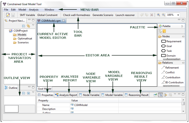


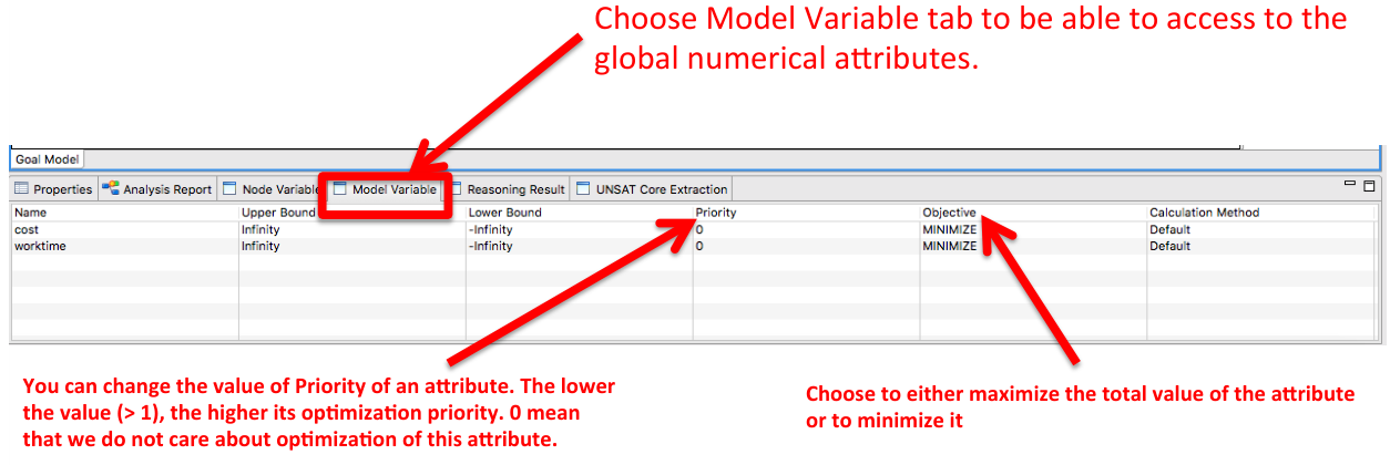


CGM-Tool provides support for modelling and reasoning on CGMs. Technically, CGM-Tool is a standalone application written in Java and its core is based on Eclipse RCP engine. Under the hood, it encodes CGMs and invokes the OptiMathSAT 66 6 http://optimathsat.disi.unitn.it SMT/OMT solver [39] to support reasoning on goal models. It is freely distributed as a compressed archive file for multiple platforms 77 7 http://www.cgm-tool.eu/. CGM-Tool supports:
- Specification of projects:
-
CGMs are created within the scope of project containers. A project contains a set of CGMs that can be used to generate reasoning sessions with OptiMathSAT (i.e., scenarios);
- Diagrammatic modelling:
-
the tool enables the creation (drawing) of CGMs in terms of diagrams; furthermore it enhances the modelling process by providing real-time check for refinement cycles and by reporting invalid refinement, contribution and binding links;
- Consistency/well-formedness check:
-
CGM-Tool allows for the creation of diagrams conform with the semantics of the modelling language by providing the ability to run consistency analysis on the model;
- Automated Reasoning:
-
CGM-Tool provides the automated reasoning functionalities of §5.2 by encoding the model into an SMT formula. The results of OptiMathSAT are shown directly on the model as well as in a tabular form.
One essential feature of the tool is that expressive constructs (which may be more complex and difficult to use) are only available on demand: there are easy-to-use default settings for everything, so that the user can decide the level of expressiveness he/she feels at ease with.
CGM-Tool extends the STS-Tool [32] as an RCP application by using the major frameworks shown in Figure 5: Rich Client Platform (RCP), a platform for building rich client applications, made up of a collection of low level frameworks such as OSGi, SWT, JFace and Equnix, which provide us a workbench where to get things like menus, editors and views; Graphical Editing Framework (GEF), a framework used to create graphical editors for graphical modelling tools (e.g., tool palette and figures which can be used to graphically represent the underlying data model concepts); Eclipse Modelling Framework (EMF), a modelling framework and a code generation facility for building tools and applications based on a structured data model.
With CGM-Tool, a CGM is built progressively as a sequence of scenarios, which are versions of the CGM to which the automated reasoning functionalities of the CGM-Tool can be applied. Figure 6 shows the graphical user interface (GUI) of the tool. Figures 7 and 8 show respectively how to define a numerical attribute of an element and how to set its value. Figure 9 shows how to set objective functions from the numerical attributes (e.g., set the priorities, choose the form of optimization (maximize/minimize), …). Figure 10 shows how to define the global constraints in the model. Figure 11 and Figure 12 show how to create and open a scenario. Figure 13 shows how the user assertions can be added by using the option “Force True” (element that must be included in the realization) and “Force False” (element that must not be included in the realization). Figure 14 shows how to automatically generate a realization for the current scenario by invoking the automated-reasoning functionalities.
7 Scalability of the Reasoning Tool
We address the issue of the scalability of the automated-reasoning functionalities of §5.2 wrt. the size of CGMs, by providing an empirical evaluation of the performance of CGM-Tool on increasingly-large CGMs. (For the sake of readability, here we provide only a qualitative description, whereas the data and plots are reported in an Appendix.) As in §3, all experiments have been run on a MacBook Air laptop, Intel Core i5 1.8 GHz, 2 cores, 256 KB L2 Cache per Core, 3 MB L3 Cache, 4GB RAM.
For the readers’ convenience, a compressed directory containing all the material to reproduce these experiments (models, tools, scripts, etc.) is available at http://www.cgm-tool.eu/experiment-version/.
We consider first the schedule-meeting CGM of §3 as a seed model. The model consists in goals –among which there are mandatory requirement, nice-to-have requirements, and tasks– plus refinements and domain assumptions, totaling nodes. The CGM contains also numerical objectives: , , and . The user-defined objectives and involve respectively and tasks and no requirement, whilst the pre-defined attributes involves tasks plus all non-mandatory requirements. This involves rational variables (recall Remark 7). There are also three binary preference relations (18).
In the example reported in §3 with different configurations, the tool returned the optimal solutions in negligible time (all took less than seconds). This is not surprising: as mentioned in §2.1, in previous empirical evaluation of OMT-encoded problems from formal verification, OptiMathSAT successfully handled optimization problems with up to thousands Boolean/rational variables [38], so that hand-made CGMs resulting into SMT formulas with few tens of Boolean and rational variables, like that in §3, are not a computational challenge.
In perspective, since CGM-Tool is supposed to be used to design CGMs representing possibly-large projects, we wonder how its automated-reasoning functionalities will scale on large models. To do this, we choose to build benchmark CGMs of increasing size, by combining different instances of the schedule-meeting CGM of §3 in various ways, and testing them with different combination of objectives.
7.1 Experiment Setup.
In all our experiments CGMs were produced as follows, according to three positive integer parameters , , and , and some choices of objectives.
Given and , we pick distinct instances of the schedule-meeting CGM of §3, each with a fresh set of Boolean labels and rational variables, we create an artificial root goal with only one refinement whose source goals are the mandatory requirements “” of each CGM instance. Hence, the resulting CGM has nodes and rational variables (see Figure 16). In another group of experiments (see Figure 16) we dropped the non-mandatory requirements and their 4 direct sub-tasks, so that each instance contains goals, domain assumptions and refinements, and the resulting CGM has nodes and rational variables.
Then we randomly add contribution relations “” and conflict relations “” between tasks belonging to different instances. When binary preference relations are involved (see below), we also randomly add binary preference relations, each involving two refinements of one same goal.
In each group of experiments we fix the definition of the objectives and we set the value of (and when it applies), and increase the values of . For every choice of , we automatically 88 8 To perform this test automatically, we developed an automated problem generator/manipulator which interfaces directly with the internal data structure representing the CGMs inside CGM-Tool. generate 100 instances of random problems as in the above schema, which we feed to our tool, and collect the median CPU times over the solved instances –including both encoding and solving times– as well as the number of unrealizable instances as well as the number of instances which OptiMathSAT could not solve within a timeout of seconds.
Notice that, following some ideas from a different context [20, 33], the parameters , and have been chosen so that to allow us to increase monotonically and tune some essential features of the CGMs under test, which may significantly influence the performances. E.g.,
- •
increases linearly the number of Boolean and rational variables,
- •
(and, to some extent, ) increases the connectivity of the graph and the ratio between unrealizable and realizable CGMs.
- •
Importantly, and also play an essential role in drastically reducing the symmetry of the resulting CGMs, and insert some degree of randomness.
Another important parameter, which we borrowed from the schedule-meeting CGM, is the number of Boolean atoms per objective.
Remark 8
We are aware that the CGMs produced with this approach may not represent realistic problems. However, we stress the fact that here we focus only on providing a test on the scalability of our automated-reasoning functionalities.
7.2 Results.
We run two groups of experiments in which we focus on optimizing, respectively:
- •
numerical attributes, like cost, work-time, penalty/rewards;
- •
discrete features, like the number of binary preferences, of want-to-have requirements and of tasks to accomplish.
In the first group of experiments we consider the reduced version of the CGMs (i.e. without nice-to-have requirements) without random binary preference relations. We fix . In each setting, we run experiments on three functionalities:
- a.
plain realizability check (without objectives),
- b.
single-objective optimization on , , and respectively,
- c.
lexicographic optimization respectively on and on .
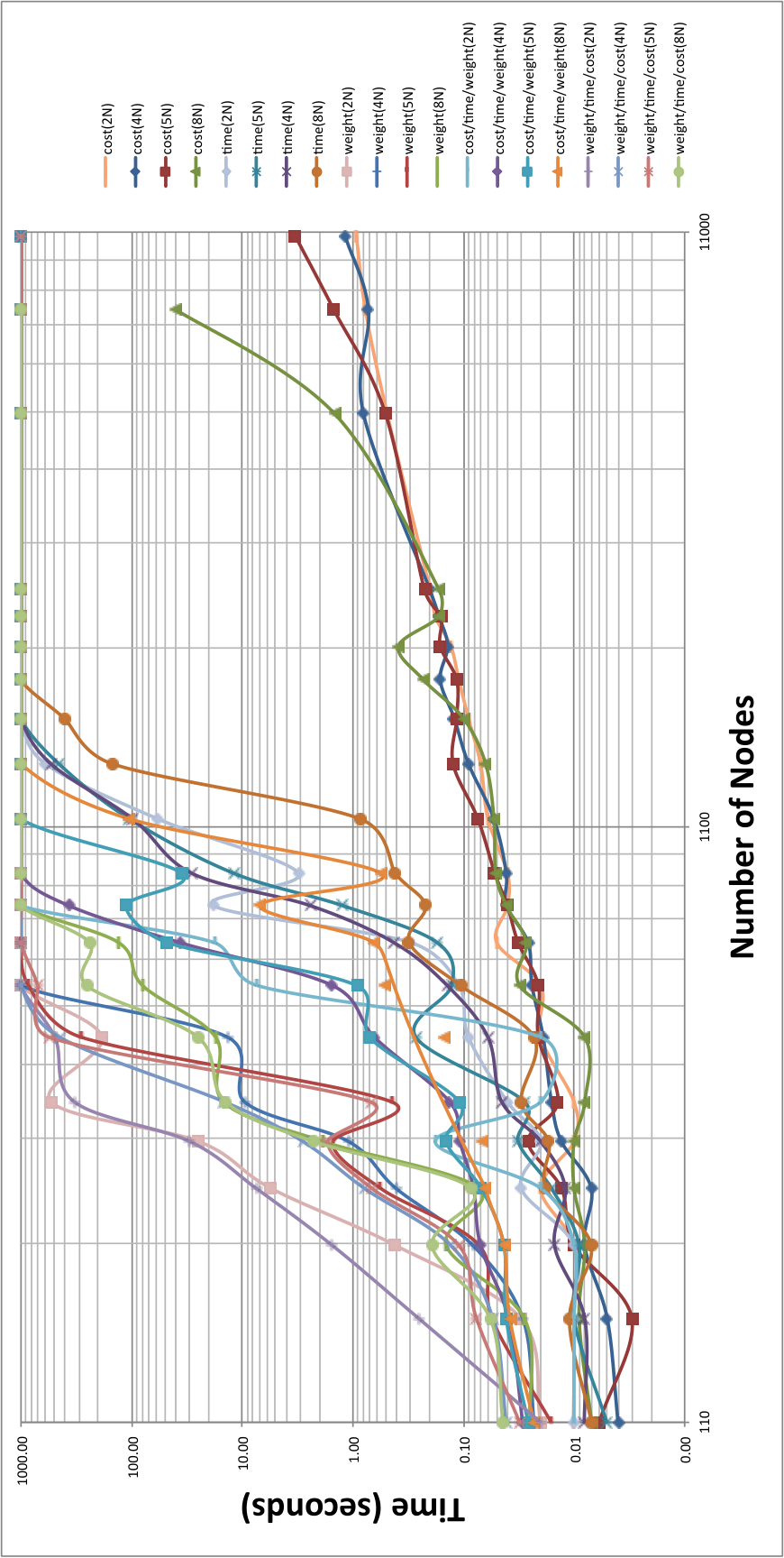
Figure 17 shows the overall median CPU time over the solved instances of the first group of experiments, which are plotted against the total number of nodes of the CGM under test. 99 9 The choice of using the total number of nodes for the X axis in all our plots aims at providing an eye-catching indication of the actual size of the CGMs under test. (For more details about the experiment data and the median CPU time over the solved instances for each special case please see Figures 20-26 in the Appendix.)
First, we notice that checking the realizability of the CGM, that is, finding one realization or verifying there is none, requires negligible time, even with huge CGMs ( nodes, rational variables) and even when the CGM is not realizable. Second, the time taken to find optimal solutions on single objectives seem to depend more on the number of variables in the objective than on the actual size of the CGM: for ( variables) the solver can find optimum solutions very quickly even with huge CGMs ( nodes, rational variables) whilst with ( variables) it can handle problems of up to nodes and rational variables. Third, lexicographic optimization takes more time than single-objective optimization, but the time mostly depends on the first objective in the list.
In the second group of experiments we consider the full version of the CGMs (with nice-to-have requirements) and introduce the random binary preference relations. We fix and we run different experiments for , and . In each setting, we run experiments on three functionalities:
- a.
plain realizability check (without objectives),
- b.
lexicographic optimization on (PRT),
- c.
lexicographic optimization on (RPT).
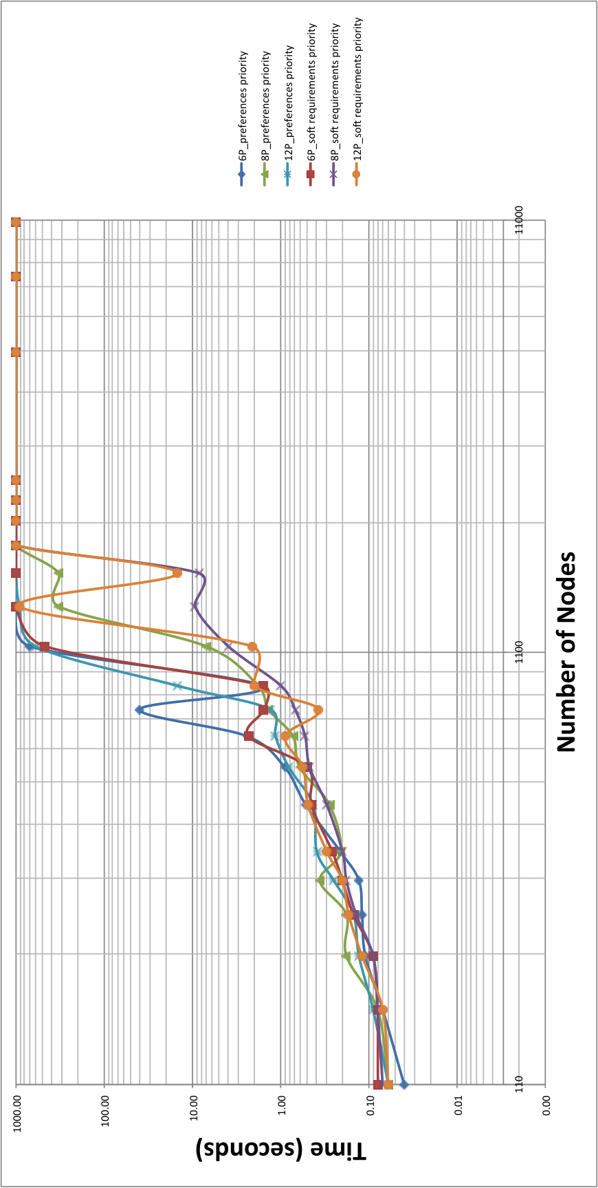
Figure 18 shows the overall median CPU time over the solved instances of the second group of experiments. (For more details about the experiment data and the median CPU time over the solved instances for each special case please see Figures 27-32 in the Appendix.)
First, checking realizability is accomplished in negligible time even with huge CGMs ( nodes, rational variables), as before. Second, we notice that optimal solutions, even with a three-level lexicographic combination of objectives, can be found with large CGMs ( nodes, rational variables).
On the negative side, for some problems, in particular large ones with objectives involving large amounts of elements, we notice that the search for the optimal realization could not be accomplished within the timeout.
To this extent, a few remarks are in order.
First, when interrupted by a timeout, OptiMathSAT can be instructed to return the current best solution. Since OptiMathSAT typically takes most of its time in fine-tuning the optimum and in checking there is no better one (see [38]), we envisage that good sub-optimal solutions can be found even when optimal ones are out of reach.
Second, our CGMs are very large in breadth and small in depth, with a dominating percentage of tasks over the total number of goals. We envisage that this may have made the number of variables in the sums defining and unrealistically large wrt. the total size of the CGMs. This underscores the need for further experimentation to confirm the scalability of our proposal.
Third, in our experiments we did not consider user assertions which, if considered, would force deterministic assignments and hence reduce drastically the size of the OMT search space.
Fourth, OMT is a recent technology [37] which is progressing at a very high pace, so that it is reasonable to expect further performance improvements for the future versions of OMT tools. In particular, a recent enhancement for handling Pseudo-Boolean cost functions as in (21) has provided interesting preliminary results [41].
Overall, our evaluation showed that CGM-Tool always checks the realizability of huge CGMs in negligible time and finds optimal realizations on problems whose size ranges from few hundreds to thousands of nodes, mostly depending on the number of variables involved in the objective functions.
|
Experiment |
Number of Instances |
Number of Replicas (N) |
Number of Goals |
Number of Refinements |
Number of Domain Assumptions |
Total Number of Nodes |
Number of Rational Variables |
| 1 | 100 | 2 | 49 | 37 | 4 | 90 | 52 |
| 2 | 100 | 3 | 73 | 55 | 6 | 134 | 78 |
| 3 | 100 | 4 | 97 | 73 | 8 | 178 | 104 |
| 4 | 100 | 5 | 121 | 91 | 10 | 222 | 130 |
| 5 | 100 | 6 | 145 | 109 | 12 | 266 | 156 |
| 6 | 100 | 7 | 169 | 127 | 14 | 310 | 182 |
| 7 | 100 | 9 | 217 | 163 | 18 | 398 | 234 |
| 8 | 100 | 11 | 265 | 199 | 22 | 486 | 286 |
| 9 | 100 | 13 | 313 | 235 | 26 | 574 | 338 |
| 10 | 100 | 15 | 361 | 271 | 30 | 662 | 390 |
| 11 | 100 | 17 | 409 | 307 | 34 | 750 | 442 |
| 12 | 100 | 21 | 505 | 379 | 42 | 926 | 546 |
| 13 | 100 | 26 | 625 | 469 | 52 | 1146 | 676 |
| 14 | 100 | 31 | 745 | 559 | 62 | 1366 | 806 |
| 15 | 100 | 36 | 865 | 649 | 72 | 1586 | 936 |
| 16 | 100 | 41 | 985 | 739 | 82 | 1806 | 1066 |
| 17 | 100 | 46 | 1105 | 829 | 92 | 2026 | 1196 |
| 18 | 100 | 51 | 1225 | 919 | 102 | 2246 | 1326 |
| 19 | 100 | 101 | 2425 | 1819 | 202 | 4446 | 2626 |
| 20 | 100 | 151 | 3625 | 2719 | 302 | 6646 | 3926 |
| 21 | 100 | 201 | 4825 | 3619 | 402 | 8846 | 5226 |
|
Experiment |
Number of Instances |
Number of Replicas (N) |
Number of Goals |
Number of Refinements |
Number of Domain Assumptions |
Total Number of Nodes |
Number of Rational Variables |
| 1 | 100 | 2 | 65 | 41 | 4 | 110 | 60 |
| 2 | 100 | 3 | 97 | 61 | 6 | 164 | 90 |
| 3 | 100 | 4 | 129 | 81 | 8 | 218 | 120 |
| 4 | 100 | 5 | 161 | 101 | 10 | 272 | 150 |
| 5 | 100 | 6 | 193 | 121 | 12 | 326 | 180 |
| 6 | 100 | 7 | 225 | 141 | 14 | 380 | 210 |
| 7 | 100 | 9 | 289 | 181 | 18 | 488 | 270 |
| 8 | 100 | 11 | 353 | 221 | 22 | 596 | 330 |
| 9 | 100 | 13 | 417 | 261 | 26 | 704 | 390 |
| 10 | 100 | 15 | 481 | 301 | 30 | 812 | 450 |
| 11 | 100 | 17 | 545 | 341 | 34 | 920 | 510 |
| 12 | 100 | 21 | 673 | 421 | 42 | 1136 | 630 |
| 13 | 100 | 26 | 833 | 521 | 52 | 1406 | 780 |
| 14 | 100 | 31 | 993 | 621 | 62 | 1676 | 930 |
| 15 | 100 | 36 | 1151 | 721 | 72 | 1946 | 1080 |
| 16 | 100 | 41 | 1313 | 821 | 82 | 2216 | 1230 |
| 17 | 100 | 46 | 1473 | 921 | 92 | 2486 | 1380 |
| 18 | 100 | 51 | 1633 | 1021 | 102 | 2756 | 1530 |
| 19 | 100 | 101 | 3233 | 2021 | 202 | 5456 | 3030 |
| 20 | 100 | 151 | 4833 | 3021 | 302 | 8156 | 4530 |
| 21 | 100 | 201 | 6433 | 4021 | 402 | 10856 | 6030 |
8 Related work
We next offer a quick overview of, and comparison with some the state of the art goal-oriented modelling languages. [24], [23], and [6] provide better and deeper comparisons on requirements modelling languages and the goal-oriented approach, including their advantages and limitations.
KAOS. KAOS [11] supports a rich ontology for requirements that goes well beyond goals, as well as a Linear Temporal Logic (LTL)-grounded formal language for constraints. This language is coupled with a concrete methodology for capturing and analyzing requirements problems. KAOS supports a number of analysis techniques, including obstacle, inconsistency and probabilistic goal analysis. However, unlike our proposal, KAOS does not support nice-to-have requirements and preferences, nor does it exploit SAT/SMT solver technologies for scalability.
Sebastiani et al.. Sebastiani et al. [18, 36] propose a formal goal modelling language that supports scalable reasoning using SAT-solving techniques. Our proposal subsumes that work in many ways, including a more expressive language and much more advanced SMT/OMT-solving technology.
There is one construct of [18, 36] that was left out of the CGM language: and contributions from goals to goals. There are several reasons for this decision. In un-constrained) goal models, formalizing (, ) contributions require a 4-value logic (fully/partially satisfied/denied). In principle our CGM framework could be extended to such a logic, with the following drawbacks:
- (a)
The size of the Boolean search space would extend from to . Given that reasoning functionality in this paper are much more sophisticated and computationally more demanding than those in our earlier papers, this might drastically reduce the efficiency of the approach.
- (b)
Unlike standard 2-value logic, which allows us to give a clear semantics of “realization”, without any vagueness, it is not obvious to us what a “realization” could be in such logic. (E.g., should realizations admit partially satisfied/denied tasks/requirements/assumptions? If yes, how should an user interpret a partially-satisfied/denied requirement/task/assumption in a realization returned by the system? In which sense a realization involving partial values can be considered “optimal” or “optimum”?
There are other differences between the two proposals. In CGMs, we have made and/or-decompositions explicit by making refinement a first class citizen that can be named and talked about (see Figure 4 and Remark 5). Moreover, unlike with [18, 36], we have a backbone and/or DAG, where arbitrary constraints can be added. This DAG is such that a non-leaf goal is equivalent to the disjunction (“or”) of its refinements, and each refinement is equivalent to the conjunction (“and”) of its source goals. Relation edges, constraints and assertions further constrain this structure.
and Tropos. [43] focuses on modelling actors for a requirements engineering problem (stakeholders, users, analysts, etc.), their goals and inter-dependencies. provides two complementary views of requirements: the Actor Strategic Dependency Model (SD model) and the Actor Strategic Rationale Model (SR model). Typically, SD models are used to analyze alternative networks of delegations among actors for fulfilling stakeholder goals, whilst SR models are used to explore alternative ways of fulfilling a single actor’s goals. is expressively lightweight, intended for early stages of requirements analysis, and did not support formal reasoning until recent thesis work by Horkoff [19]. Tropos [7] is a requirements-driven agent-oriented software development methodology founded on . Goal models can be formalized in Tropos by using Formal Tropos [17], an extension of that supports LTL for formalizing constraints. The main deficiencies of this work relative to our proposal is that Formal Tropos is expressive but not scalable.
Techne and Liaskos. Techne [22] is a recent proposal for a family of goal-modelling languages that supports nice-to-have goals and preferences, but it is strictly propositional and uses hand-crafted algorithms, and therefore does not support optimization goals. [15] constitutes a first attempt to reason with nice-to-have requirements (aka preferences). The scalability experiments conducted used the SAT solver of Sebastiani et al. [36] and added local search algorithms to deal with preferences. All experiments where conducted on a model with about 500 elements and the search algorithms returned maximal consistent solution but also near-solutions. [12] focuses on finding new solutions for a goal model that has changed (new goals were added/removed), such that the change minimizes development effort (EvoR1) or maximizes familiarity (EvoR2). Note that EvoR1, EvoR2 are evolution requirements. The paper uses a Truth-Maintenance System (TMS) and builds algorithms on top for finding solutions to EvoR1, EvoR2 that “repair” the previous solution and construct a new one. The search algorithms would need to be redone if we used different evolution algorithms, unlike the CGM tool where you can formally express EvoR1, EvoR2 or variants, and search is handle by the backend OMT/SMT solver. [14, 13] continue the study of reasoning with Techne models and use SAT solvers and hand-crafted search algorithms to establish scalability for models size O(1K). Nevertheless the resulting tools from this work still can’t handle quantitative optimization problems and other features of CGMs.
Liaskos [26, 25] has proposed extensions to qualitative goal models to support nice-to-have goals and preferences, as well as decision-theoretic concepts such as utility. This proposal is comparable to our proposal in this paper, but uses AI reasoners for reasoning (AI planners and GOLOG) and, consequently, does not scale very well relative to our proposal.
Feature Models. Feature models [10] share many similarities with goal models: they are hierarchically structured, with AND/OR refinements, constraints and attributes. However, each feature represents a bundle of functionality or quality and as such, feature models are models of software configurations, not requirements. Moreover, reasoning techniques for feature models are limited relative to their goal model cousins.
Search-Based Software Engineering. Scalable reasoning for optimization problems has been studied by Harman et al in the context of formalizing and solving the next release problem [44]: given a set of preferences with associated cost and customer value attributes, select a subset of preferences to be included in the next release that optimizes given attributes. That work uses genetic algorithms and other search techniques that may return close-to-optimal solutions and use heuristics (meaning that reasoning is not complete).
9 Conclusions and Future Work
We have proposed, an expressive goal-based modelling language for requirements that supports the representation of nice-to-have requirements, preferences, optimization requirements, constraints and more. Moreover, we have exploited automated reasoning solvers in order to develop a tool that supports sound and complete reasoning with respect to such goal models, and scales well to goal models with thousands of elements. Our proposal advances the state-of-the-art on goal modelling and reasoning with respect to both expressiveness and scalability of reasoning.
The contributions of this work are being exploited in several directions. [4] has proposed an expressive modelling framework for the next release problem that is founded on the same OMT/SMT solver technology as this work. [1] has offered a formalization of the next adaptation problem that chooses a next adaptation for an adaptive software system that minimizes the degree of failure over existing requirements. And [30] has exploited CGMs to capture evolution requirements, such as “System evolution shall minimize implementation costs” and showed how to conduct scalable reasoning over models that include such requirements.
As future work, we have planned to do an empirical validation of the CGM-Tool with modelers and domain experts. We are currently working in this direction within our research group with PhD students and post-docs who are expert in the modelling field. Next, we will extend the validation to industrial experts of different domains. We have also planned to do different case studies with real-life-complex-large-scale goal models of a specific domain, such as Air-Traffic Control Management, healthcare, and smart cities and smart environments.
Our proposal does not address another notorious scalability problem of goal models, namely scalability-of-use. Goal models have been shown empirically to become more difficult to conceptualize and comprehend as they grow in size [16], and therefore become unwieldy for use. As with other kinds of artifacts (e.g., programs, ontologies) where scalability-of-use is an issue, the solution lies in introducing modularization facilities that limit interactions between model elements and make the resulting models easier to understand and evolve. This is an important problem on our agenda for future research on goal models.
Acknowledgements.
We would like to thank Dagmawi Neway for his technical support in developing CGM-Tool, and Patrick Trentin for assistance with the usage of OptiMathSAT.References
- (1) Angelopoulos, K., Aydemir, F., Giorgini, P., Mylopoulos, J.: Solving the next adaptation problem with prometheus. RCIS (2016)
- (2) Anton, A.I.: Goal-based requirements analysis. In: Proceedings of the 2nd International Conference on Requirements Engineering, ICRE ’96, pp. 136–. IEEE Computer Society (1996)
- (3) Anton, A.I., Potts, C.: The use of goals to surface requirements for evolving systems. In: Proceedings of the 20th international conference on Software engineering, ICSE ’98, pp. 157–166. IEEE Computer Society (1998)
- (4) Aydemir, F., Mekuria, D., Giorgini, P., Mylopoulos, J.: Scalable solutions to the next release problem: A goal-oriented perspective (2016). Under submission.
- (5) Barrett, C.W., Sebastiani, R., Seshia, S.A., Tinelli, C.: Satisfiability Modulo Theories. In: Handbook of Satisfiability, chap. 26, pp. 825–885. IOS Press (2009)
- (6) Borgida, A., Dalpiaz, F., Horkoff, J., Mylopoulos, J.: Requirements models for design- and runtime: A position paper. In: Proceedings of the 5th International Workshop on Modeling in Software Engineering, MiSE ’13, pp. 62–68. IEEE Press (2013)
- (7) Castro, J., Kolp, M., Mylopoulos, J.: Towards requirements-driven information systems engineering: The tropos project. Inf. Syst. 27(6), 365–389 (2002). DOI 10.1016/S0306-4379(02)00012-1
- (8) Cimatti, A., Griggio, A., Schaafsma, B.J., Sebastiani, R.: The MathSAT 5 SMT Solver. In: Tools and Algorithms for the Construction and Analysis of Systems, TACAS’13., LNCS, vol. 7795, pp. 95–109. Springer (2013)
- (9) Cimatti, A., Griggio, A., Sebastiani, R.: Computing Small Unsatisfiable Cores in SAT Modulo Theories. Journal of Artificial Intelligence Research, JAIR 40, 701–728 (2011)
- (10) Classen, A., Boucher, Q., Heymans, P.: A text-based approach to feature modelling: Syntax and semantics of TVL. Sci. Comput. Program. 76(12), 1130–1143 (2011). DOI 10.1016/j.scico.2010.10.005
- (11) Dardenne, A., van Lamsweerde, A., Fickas, S.: Goal-directed requirements acquisition. Sci. Comput. Program. 20(1-2), 3–50 (1993)
- (12) Ernst, N.A., Borgida, A., Jureta, I.: Finding incremental solutions for evolving requirements. In: RE, pp. 15–24. IEEE (2011)
- (13) Ernst, N.A., Borgida, A., Jureta, I.J., Mylopoulos, J.: Agile requirements engineering via paraconsistent reasoning. Information Systems 43, 100 – 116 (2014). DOI http://dx.doi.org/10.1016/j.is.2013.05.008
- (14) Ernst, N.A., Borgida, A., Mylopoulos, J., Jureta, I.: Agile Requirements Evolution via Paraconsistent Reasoning. In: J. Ralyté, X. Franch, S. Brinkkemper, S. Wrycza (eds.) CAiSE, Lecture Notes in Computer Science, vol. 7328, pp. 382–397. Springer (2012)
- (15) Ernst, N.A., Mylopoulos, J., Borgida, A., Jureta, I.J.: Reasoning with optional and preferred requirements. In: J. Parsons, M. Saeki, P. Shoval, C. Woo, Y. Wand (eds.) Conceptual Modeling – ER 2010: 29th International Conference on Conceptual Modeling, Vancouver, BC, Canada, November 1-4, 2010. Proceedings, pp. 118–131. Springer Berlin Heidelberg, Berlin, Heidelberg (2010). DOI 10.1007/978-3-642-16373-9_9
- (16) Estrada, H., Rebollar, A.M., Pastor, O., Mylopoulos, J.: An empirical evaluation of the i* framework in a model-based software generation environment. In: E. Dubois, K. Pohl (eds.) Advanced Information Systems Engineering, 18th International Conference, CAiSE 2006, Luxembourg, Luxembourg, June 5-9, 2006, Proceedings, Lecture Notes in Computer Science, vol. 4001, pp. 513–527. Springer (2006). DOI 10.1007/11767138_34
- (17) Fuxman, A., Liu, L., Mylopoulos, J., Pistore, M., Roveri, M., Traverso, P.: Specifying and analyzing early requirements in tropos. Requir. Eng. 9(2), 132–150 (2004). DOI 10.1007/s00766-004-0191-7
- (18) Giorgini, P., Mylopoulos, J., Nicchiarelli, E., Sebastiani, R.: Formal reasoning techniques for goal models. JOURNAL OF DATA SEMANTICS 1, 1–20 (2004)
- (19) Horkoff, J.M.: Iterative, interactive analysis of agent-goal models for early requirements engineering. Ph.D. thesis, University of Toronto (2012). AAINR97565
- (20) Horrocks, I., Patel-Schneider, P.F., Sebastiani, R.: An Analysis of Empirical Testing for Modal Decision Procedures. Logic Journal of the IGPL 8(3), 293–323 (2000)
- (21) Jarvis, R., McArthur, G., Mylopoulos, J., Rodríguez-Gianolli, P., Zhou, S.: Semantic models for knowledge management. In: WISE (1), pp. 8– (2001)
- (22) Jureta, I., Borgida, A., Ernst, N.A., Mylopoulos, J.: Techne: Towards a new generation of requirements modeling languages with goals, preferences, and inconsistency handling. In: RE, pp. 115–124. IEEE Computer Society (2010)
- (23) Jureta, I., Mylopoulos, J., Faulkner, S.: Revisiting the core ontology and problem in requirements engineering. In: Proceedings of the 2008 16th IEEE International Requirements Engineering Conference, RE ’08, pp. 71–80. IEEE Computer Society (2008). DOI 10.1109/RE.2008.13
- (24) Lapouchnian, A.: Goal-Oriented Requirements Engineering: An Overview of the Current Research. Tech. rep., Department of Computer Science, University of Toronto (2005)
- (25) Liaskos, S.: On eliciting contribution measures in goal models. In: Proceedings of the 2012 IEEE 20th International Requirements Engineering Conference (RE), RE ’12, pp. 221–230. IEEE Computer Society (2012). DOI 10.1109/RE.2012.6345808
- (26) Liaskos, S., McIlraith, S.A., Sohrabi, S., Mylopoulos, J.: Integrating preferences into goal models for requirements engineering. In: RE, pp. 135–144. IEEE Computer Society (2010)
- (27) Mekuria, D.N.: Constrained goal modeling and reasoning tool’s user manual
- (28) Mylopoulos, J., Chung, L., Nixon, B.: Representing and using nonfunctional requirements: A process-oriented approach. IEEE Trans. Softw. Eng. 18(6), 483–497 (1992). DOI 10.1109/32.142871
- (29) Newell, A., Simon, H.: GPS: A program that simulates human thought. In: E.A. Feigenbaum, J. Feldman (eds.) Computers and Thought, pp. 279–293. McGraw-Hill (1963)
- (30) Nguyen, C.M., Sebastiani, R., Giorgini, P., Mylopoulos, J.: Requirements Evolution and Evolution Requirements with Constrained Goal Models. In: Proceedings of the 37nd International Conference on Conceptual Modeling, LNCS. Springer (2016)
- (31) Nieuwenhuis, R., Oliveras, A.: On SAT Modulo Theories and Optimization Problems. In: Proc SAT’06, LNCS, vol. 4121. Springer (2006)
- (32) Paja, E., Dalpiaz, F., Poggianella, M., Roberti, P., Giorgini, P.: STS-Tool: socio-technical security requirements through social commitments. In: Proceedings of the 20th IEEE International Conference on Requirements Engineering, pp. 331–332 (2012)
- (33) Patel-Schneider, P.F., Sebastiani, R.: A New General Method to Generate Random Modal Formulae for Testing Decision Procedures. Journal of Artificial Intelligence Research, (JAIR) 18, 351–389 (2003). Morgan Kaufmann
- (34) Rao, A.S., George, M.P.: BDI Agents: From Theory to Practice. In: Proceedings of the First International Conference on Multiagent Systems. AAAI (1995)
- (35) Sebastiani, R.: Lazy Satisfiability Modulo Theories. Journal on Satisfiability, Boolean Modeling and Computation, JSAT 3(3-4), 141–224 (2007)
- (36) Sebastiani, R., Giorgini, P., Mylopoulos, J.: Simple and Minimum-Cost Satisfiability for Goal Models. In: Proc. 16th International Conference on Advanced Information Systems Engineering - CAISE’04, LNCS. Springer, Riga, Latvia (2004)
- (37) Sebastiani, R., Tomasi, S.: Optimization in SMT with LA(Q) Cost Functions. In: IJCAR, LNAI, vol. 7364, pp. 484–498. Springer (2012)
- (38) Sebastiani, R., Tomasi, S.: Optimization Modulo Theories with Linear Rational Costs. ACM Transactions on Computational Logics 16(2) (2015)
- (39) Sebastiani, R., Trentin, P.: OptiMathSAT: A Tool for Optimization Modulo Theories. In: Proc. International Conference on Computer-Aided Verification, CAV 2015, LNCS, vol. 9206. Springer (2015)
- (40) Sebastiani, R., Trentin, P.: Pushing the Envelope of Optimization Modulo Theories with Linear-Arithmetic Cost Functions. In: Proc. Int. Conference on Tools and Algorithms for the Construction and Analysis of Systems, TACAS’15, LNCS, vol. 9035. Springer (2015)
- (41) Sebastiani, R., Trentin, P.: On the Benefits of Enhancing Optimization Modulo Theories with Sorting Networks for MaxSMT. In: Proceedings of the 14th International Workshop on Satisfiability Modulo Theories, SMT-2016., CEUR Workshop Proceedings (2016)
- (42) Van Lamsweerde, A.: Goal-oriented requirements engineering: A guided tour. In: Proceedings of the Fifth IEEE International Symposium on Requirements Engineering, RE ’01, pp. 249–. IEEE Computer Society (2001)
- (43) Yu, E.S.K.: Towards modeling and reasoning support for early-phase requirements engineering. In: RE ’97: Proceedings of the 3rd IEEE International Symposium on Requirements Engineering (RE’97), p. 226. IEEE Computer Society (1997)
- (44) Zhang, Y., Harman, M., Mansouri, S.A.: The multi-objective next release problem. In: Proceedings of the 9th Annual Conference on Genetic and Evolutionary Computation, GECCO ’07, pp. 1129–1137. ACM, New York, NY, USA (2007). DOI 10.1145/1276958.1277179
Appendix A Appendix: Data Tables and Plots
A.1 First Group of Experiments
| Optimum | Optimum | Optimum | Lexic. Order | Lexic. Order | |||||||||||||
|---|---|---|---|---|---|---|---|---|---|---|---|---|---|---|---|---|---|
| cost | time | weight | cost time weight | weight time cost | |||||||||||||
| (2N terms) | (5N terms) | (16N terms) | |||||||||||||||
|
Experiment |
Number of Instances |
Number of Replicas (N) |
Total Number of Nodes |
Number of Rational Variables |
% Unrealizable |
Solving Time |
Time for Proving Unrealizable |
Optimization Time |
% Timeout |
Optimization Time |
% Timeout |
Optimization Time |
% Timeout |
Optimization Time |
% Timeout |
Optimization Time |
% Timeout |
| 1 | 100 | 2 | 90 | 52 | 1 | 0.00 | 0.00 | 0.00 | 0 | 0.01 | 0 | 0.02 | 0 | 0.01 | 0 | 0.02 | 0 |
| 2 | 100 | 3 | 134 | 78 | 1 | 0.00 | 0.00 | 0.01 | 0 | 0.01 | 0 | 0.03 | 0 | 0.01 | 0 | 0.25 | 0 |
| 3 | 100 | 4 | 178 | 104 | 3 | 0.00 | 0.00 | 0.01 | 0 | 0.01 | 0 | 0.41 | 0 | 0.01 | 0 | 1.53 | 0 |
| 4 | 100 | 5 | 222 | 130 | 3 | 0.00 | 0.00 | 0.02 | 0 | 0.03 | 0 | 5.51 | 0 | 0.02 | 0 | 7.48 | 0 |
| 5 | 100 | 6 | 266 | 156 | 2 | 0.00 | 0.00 | 0.01 | 0 | 0.02 | 0 | 24.74 | 0 | 0.18 | 0 | 29.74 | 2 |
| 6 | 100 | 7 | 310 | 182 | 5 | 0.00 | 0.00 | 0.01 | 0 | 0.04 | 0 | 533.90 | 19 | 0.02 | 0 | 329.34 | 30 |
| 7 | 100 | 9 | 398 | 234 | 7 | 0.00 | 0.00 | 0.02 | 0 | 0.09 | 0 | 185.23 | 84 | 0.02 | 4 | 494.33 | 87 |
| 8 | 100 | 11 | 486 | 286 | 4 | 0.00 | 0.00 | 0.02 | 0 | 0.11 | 0 | — | — | 7.29 | 30 | — | — |
| 9 | 100 | 13 | 574 | 338 | 7 | 0.00 | 0.00 | 0.05 | 0 | 0.30 | 0 | — | — | 17.98 | 83 | — | — |
| 10 | 100 | 15 | 662 | 390 | 13 | 0.00 | 0.00 | 0.04 | 0 | 18.13 | 0 | — | — | — | — | — | — |
| 11 | 100 | 17 | 750 | 442 | 15 | 0.00 | 0.00 | 0.04 | 0 | 3.11 | 0 | — | — | — | — | — | — |
| 12 | 100 | 21 | 926 | 546 | 14 | 0.00 | 0.00 | 0.06 | 0 | 58.08 | 11 | — | — | — | — | — | — |
| 13 | 100 | 26 | 1146 | 676 | 13 | 0.00 | 0.00 | 0.07 | 0 | 600.99 | 78 | — | — | — | — | — | — |
| 14 | 100 | 31 | 1366 | 806 | 14 | 0.00 | 0.00 | 0.09 | 0 | — | — | — | — | — | — | — | — |
| 15 | 100 | 36 | 1586 | 936 | 19 | 0.00 | 0.00 | 0.11 | 0 | — | — | — | — | — | — | — | — |
| 16 | 100 | 41 | 1806 | 1066 | 26 | 0.00 | 0.00 | 0.13 | 0 | — | — | — | — | — | — | — | — |
| 17 | 100 | 46 | 2026 | 1196 | 24 | 0.00 | 0.00 | 0.18 | 0 | — | — | — | — | — | — | — | — |
| 18 | 100 | 51 | 2246 | 1326 | 32 | 0.00 | 0.00 | 0.20 | 0 | — | — | — | — | — | — | — | — |
| 19 | 100 | 101 | 4446 | 2626 | 49 | 0.00 | 0.00 | 0.49 | 0 | — | — | — | — | — | — | — | — |
| 20 | 100 | 151 | 6646 | 3926 | 68 | 0.00 | 0.00 | 0.77 | 0 | — | — | — | — | — | — | — | — |
| 21 | 100 | 201 | 8846 | 5226 | 71 | 0.00 | 0.00 | 0.93 | 0 | — | — | — | — | — | — | — | — |
| Optimum | Optimum | Optimum | Lexic. Order | Lexic. Order | |||||||||||||
|---|---|---|---|---|---|---|---|---|---|---|---|---|---|---|---|---|---|
| cost | time | weight | cost time weight | weight time cost | |||||||||||||
| (2N terms) | (5N terms) | (16N terms) | |||||||||||||||
|
Experiment |
Number of Instances |
Number of Replicas (N) |
Total Number of Nodes |
Number of Rational Variables |
% Unrealizable |
Solving Time |
Time for Proving Unrealizable |
Optimization Time |
% Timeout |
Optimization Time |
% Timeout |
Optimization Time |
% Timeout |
Optimization Time |
% Timeout |
Optimization Time |
% Timeout |
| 1 | 100 | 2 | 90 | 52 | 2 | 0.00 | 0.00 | 0.00 | 0 | 0.01 | 0 | 0.02 | 0 | 0.03 | 0 | 0.04 | 0 |
| 2 | 100 | 3 | 134 | 78 | 1 | 0.00 | 0.00 | 0.01 | 0 | 0.01 | 0 | 0.03 | 0 | 0.04 | 0 | 0.05 | 0 |
| 3 | 100 | 4 | 178 | 104 | 2 | 0.00 | 0.00 | 0.01 | 0 | 0.02 | 0 | 0.08 | 0 | 0.06 | 0 | 0.13 | 0 |
| 4 | 100 | 5 | 222 | 130 | 4 | 0.00 | 0.00 | 0.01 | 0 | 0.01 | 0 | 0.41 | 0 | 0.08 | 0 | 0.79 | 0 |
| 5 | 100 | 6 | 266 | 156 | 7 | 0.00 | 0.00 | 0.01 | 0 | 0.02 | 0 | 1.09 | 0 | 0.11 | 0 | 2.82 | 0 |
| 6 | 100 | 7 | 310 | 182 | 7 | 0.00 | 0.00 | 0.02 | 0 | 0.05 | 0 | 9.53 | 4 | 0.13 | 0 | 14.47 | 4 |
| 7 | 100 | 9 | 398 | 234 | 7 | 0.00 | 0.00 | 0.02 | 0 | 0.06 | 0 | 13.54 | 56 | 0.64 | 0 | 447.13 | 67 |
| 8 | 100 | 12 | 486 | 286 | 10 | 0.00 | 0.00 | 0.02 | 0 | 0.14 | 0 | — | — | 1.53 | 5 | — | — |
| 9 | 100 | 13 | 574 | 338 | 9 | 0.00 | 0.00 | 0.03 | 0 | 0.43 | 0 | — | — | 36.78 | 23 | — | — |
| 10 | 100 | 15 | 662 | 390 | 11 | 0.00 | 0.00 | 0.04 | 0 | 2.42 | 0 | — | — | 368.94 | 55 | — | — |
| 11 | 100 | 17 | 750 | 442 | 9 | 0.00 | 0.00 | 0.04 | 0 | 28.45 | 0 | — | — | — | — | — | — |
| 12 | 100 | 21 | 926 | 546 | 15 | 0.00 | 0.00 | 0.05 | 0 | 97.86 | 2 | — | — | — | — | — | — |
| 13 | 100 | 26 | 1146 | 676 | 22 | 0.00 | 0.00 | 0.09 | 0 | 537.73 | 62 | — | — | — | — | — | — |
| 14 | 100 | 31 | 1366 | 806 | 25 | 0.00 | 0.00 | 0.12 | 0 | — | — | — | — | — | — | — | — |
| 15 | 100 | 36 | 1586 | 936 | 27 | 0.00 | 0.00 | 0.16 | 0 | — | — | — | — | — | — | — | — |
| 16 | 100 | 41 | 1806 | 1066 | 32 | 0.00 | 0.00 | 0.14 | 0 | — | — | — | — | — | — | — | — |
| 17 | 100 | 46 | 2026 | 1196 | 36 | 0.00 | 0.00 | 0.17 | 0 | — | — | — | — | — | — | — | — |
| 18 | 100 | 51 | 2246 | 1326 | 40 | 0.00 | 0.00 | 0.20 | 0 | — | — | — | — | — | — | — | — |
| 19 | 100 | 101 | 4446 | 2626 | 55 | 0.00 | 0.00 | 0.80 | 0 | — | — | — | — | — | — | — | — |
| 20 | 100 | 151 | 6646 | 3926 | 77 | 0.00 | 0.00 | 0.72 | 0 | — | — | — | — | — | — | — | — |
| 21 | 100 | 201 | 8846 | 5226 | 85 | 0.00 | 0.00 | 1.18 | 0 | — | — | — | — | — | — | — | — |
| Optimum | Optimum | Optimum | Lexic. Order | Lexic. Order | |||||||||||||
|---|---|---|---|---|---|---|---|---|---|---|---|---|---|---|---|---|---|
| cost | time | weight | cost time weight | weight time cost | |||||||||||||
| (2N terms) | (5N terms) | (16N terms) | |||||||||||||||
|
Experiment |
Number of Instances |
Number of Replicas (N) |
Total Number of Nodes |
Number of Rational Variables |
% Unrealizable |
Solving Time |
Time for Proving Unrealizable |
Optimization Time |
% Timeout |
Optimization Time |
% Timeout |
Optimization Time |
% Timeout |
Optimization Time |
% Timeout |
Optimization Time |
% Timeout |
| 1 | 100 | 2 | 90 | 52 | 4 | 0.00 | 0.00 | 0.01 | 0 | 0.01 | 0 | 0.02 | 0 | 0.03 | 0 | 0.03 | 0 |
| 2 | 100 | 3 | 134 | 78 | 3 | 0.00 | 0.00 | 0.00 | 0 | 0.01 | 0 | 0.06 | 0 | 0.04 | 0 | 0.08 | 0 |
| 3 | 100 | 4 | 178 | 104 | 6 | 0.00 | 0.00 | 0.01 | 0 | 0.01 | 0 | 0.07 | 0 | 0.04 | 0 | 0.11 | 0 |
| 4 | 100 | 5 | 222 | 130 | 6 | 0.00 | 0.00 | 0.01 | 0 | 0.02 | 0 | 0.56 | 0 | 0.07 | 0 | 0.67 | 0 |
| 5 | 100 | 6 | 266 | 156 | 7 | 0.00 | 0.00 | 0.03 | 0 | 0.03 | 0 | 1.51 | 0 | 0.14 | 0 | 1.69 | 0 |
| 6 | 100 | 7 | 310 | 182 | 5 | 0.00 | 0.00 | 0.01 | 0 | 0.03 | 0 | 0.45 | 0 | 0.11 | 0 | 0.69 | 0 |
| 7 | 100 | 9 | 398 | 234 | 7 | 0.00 | 0.00 | 0.02 | 0 | 0.27 | 0 | 284.79 | 31 | 0.71 | 0 | 557.00 | 36 |
| 8 | 100 | 11 | 486 | 286 | 9 | 0.00 | 0.00 | 0.02 | 0 | 0.13 | 0 | 852.66 | 80 | 0.92 | 0 | 705.92 | 85 |
| 9 | 100 | 13 | 574 | 338 | 17 | 0.00 | 0.00 | 0.03 | 0 | 0.17 | 0 | — | — | 47.55 | 9 | — | — |
| 10 | 100 | 15 | 662 | 390 | 14 | 0.00 | 0.00 | 0.04 | 0 | 1.23 | 0 | — | — | 111.58 | 28 | — | — |
| 11 | 100 | 17 | 750 | 442 | 13 | 0.00 | 0.00 | 0.05 | 0 | 11.87 | 0 | — | — | 35.31 | 56 | — | — |
| 12 | 100 | 21 | 926 | 546 | 24 | 0.00 | 0.00 | 0.07 | 0 | 104.67 | 0 | — | — | — | — | — | — |
| 13 | 100 | 26 | 1146 | 676 | 27 | 0.00 | 0.00 | 0.12 | 0 | 455.20 | 51 | — | — | — | — | — | — |
| 14 | 100 | 31 | 1366 | 806 | 32 | 0.00 | 0.00 | 0.12 | 0 | — | — | — | — | — | — | — | — |
| 15 | 100 | 36 | 1586 | 936 | 33 | 0.00 | 0.00 | 0.12 | 0 | — | — | — | — | — | — | — | — |
| 16 | 100 | 41 | 1806 | 1066 | 33 | 0.00 | 0.00 | 0.16 | 0 | — | — | — | — | — | — | — | — |
| 17 | 100 | 46 | 2026 | 1196 | 53 | 0.00 | 0.00 | 0.16 | 0 | — | — | — | — | — | — | — | — |
| 18 | 100 | 51 | 2246 | 1326 | 48 | 0.00 | 0.00 | 0.23 | 0 | — | — | — | — | — | — | — | — |
| 19 | 100 | 101 | 4446 | 2626 | 73 | 0.00 | 0.00 | 0.51 | 0 | — | — | — | — | — | — | — | — |
| 20 | 100 | 151 | 6646 | 3926 | 76 | 0.00 | 0.00 | 3.33 | 0 | — | — | — | — | — | — | — | — |
| 21 | 100 | 201 | 8846 | 5226 | 93 | 0.00 | 0.00 | 1.49 | 0 | — | — | — | — | — | — | — | — |
| Optimum | Optimum | Optimum | Lexic. Order | Lexic. Order | |||||||||||||
|---|---|---|---|---|---|---|---|---|---|---|---|---|---|---|---|---|---|
| cost | time | weight | cost time weight | weight time cost | |||||||||||||
| (2N terms) | (5N terms) | (16N terms) | |||||||||||||||
|
Experiment |
Number of Instances |
Number of Replicas (N) |
Total Number of Nodes |
Number of Rational Variables |
% Unrealizable |
Solving Time |
Time for Proving Unrealizable |
Optimization Time |
% Timeout |
Optimization Time |
% Timeout |
Optimization Time |
% Timeout |
Optimization Time |
% Timeout |
Optimization Time |
% Timeout |
| 1 | 100 | 2 | 90 | 52 | 10 | 0.00 | 0.00 | 0.01 | 0 | 0.01 | 0 | 0.03 | 0 | 0.02 | 0 | 0.04 | 0 |
| 2 | 100 | 3 | 134 | 78 | 15 | 0.00 | 0.00 | 0.01 | 0 | 0.01 | 0 | 0.03 | 0 | 0.04 | 0 | 0.06 | 0 |
| 3 | 100 | 4 | 178 | 104 | 9 | 0.00 | 0.00 | 0.01 | 0 | 0.01 | 0 | 0.14 | 0 | 0.04 | 0 | 0.19 | 0 |
| 4 | 100 | 5 | 222 | 130 | 11 | 0.00 | 0.00 | 0.01 | 0 | 0.02 | 0 | 0.07 | 0 | 0.06 | 0 | 0.09 | 0 |
| 5 | 100 | 6 | 266 | 156 | 21 | 0.00 | 0.00 | 0.01 | 0 | 0.03 | 0 | 1.85 | 0 | 0.07 | 0 | 2.25 | 0 |
| 6 | 100 | 7 | 310 | 182 | 24 | 0.00 | 0.00 | 0.01 | 0 | 0.02 | 0 | 14.71 | 0 | 0.10 | 0 | 14.11 | 0 |
| 7 | 100 | 9 | 398 | 234 | 33 | 0.00 | 0.00 | 0.01 | 0 | 0.11 | 0 | 17.37 | 1 | 0.15 | 0 | 25.14 | 1 |
| 8 | 100 | 11 | 486 | 286 | 23 | 0.00 | 0.00 | 0.03 | 0 | 0.31 | 0 | 79.55 | 19 | 0.51 | 0 | 253.57 | 28 |
| 9 | 100 | 13 | 574 | 338 | 28 | 0.00 | 0.00 | 0.03 | 0 | 0.22 | 0 | 131.37 | 55 | 0.64 | 0 | 240.96 | 59 |
| 10 | 100 | 15 | 662 | 390 | 36 | 0.00 | 0.00 | 0.04 | 0 | 0.41 | 0 | — | — | 6.89 | 0 | — | — |
| 11 | 100 | 17 | 750 | 442 | 20 | 0.00 | 0.00 | 0.05 | 0 | 0.86 | 0 | — | — | 0.56 | 1 | — | — |
| 12 | 100 | 21 | 926 | 546 | 48 | 0.00 | 0.00 | 0.05 | 0 | 149.86 | 7 | — | — | 104.81 | 17 | — | — |
| 13 | 100 | 26 | 1146 | 676 | 43 | 0.00 | 0.00 | 0.06 | 0 | 406.31 | 23 | — | — | — | — | — | — |
| 14 | 100 | 31 | 1366 | 806 | 61 | 0.00 | 0.00 | 0.10 | 0 | — | — | — | — | — | — | — | — |
| 15 | 100 | 36 | 1586 | 936 | 67 | 0.00 | 0.00 | 0.23 | 0 | — | — | — | — | — | — | — | — |
| 16 | 100 | 41 | 1806 | 1066 | 71 | 0.00 | 0.00 | 0.39 | 0 | — | — | — | — | — | — | — | — |
| 17 | 100 | 46 | 2026 | 1196 | 77 | 0.00 | 0.00 | 0.17 | 0 | — | — | — | — | — | — | — | — |
| 18 | 100 | 51 | 2246 | 1326 | 75 | 0.00 | 0.00 | 0.17 | 0 | — | — | — | — | — | — | — | — |
| 19 | 100 | 101 | 4446 | 2626 | 98 | 0.00 | 0.00 | 1.47 | 0 | — | — | — | — | — | — | — | — |
| 20 | 100 | 151 | 6646 | 3926 | 97 | 0.00 | 0.00 | 40.11 | 0 | — | — | — | — | — | — | — | — |
| 21 | 100 | 201 | 8846 | 5226 | 100 | 0.00 | 0.00 | — | — | — | — | — | — | — | — | — | — |


A.2 Second Group of Experiments
| Lexic. Order PRT | Lexic. Order RPT | ||||||||||
|
Experiment |
Number of Instances. |
Number of Replicas (N) |
Total Number of Nodes |
Number of Rational Variables |
% Unrealizable |
Solving Time |
Time for Proving Unrealizable |
Optimization Time |
% Timeout |
Optimization Time |
% Timeout |
| 1 | 100 | 2 | 110 | 60 | 1 | 0.00 | 0.00 | 0.04 | 0 | 0.08 | 0 |
| 2 | 100 | 3 | 164 | 90 | 2 | 0.00 | 0.00 | 0.07 | 0 | 0.08 | 0 |
| 3 | 100 | 4 | 218 | 120 | 1 | 0.00 | 0.00 | 0.11 | 0 | 0.09 | 0 |
| 4 | 100 | 5 | 272 | 150 | 3 | 0.00 | 0.00 | 0.12 | 0 | 0.15 | 0 |
| 5 | 100 | 6 | 326 | 180 | 2 | 0.00 | 0.00 | 0.13 | 0 | 0.20 | 0 |
| 6 | 100 | 7 | 380 | 210 | 3 | 0.00 | 0.00 | 0.21 | 0 | 0.26 | 0 |
| 7 | 100 | 9 | 488 | 270 | 2 | 0.00 | 0.00 | 0.52 | 0 | 0.45 | 0 |
| 8 | 100 | 11 | 596 | 330 | 7 | 0.00 | 0.00 | 0.90 | 0 | 0.50 | 0 |
| 9 | 100 | 13 | 704 | 390 | 8 | 0.00 | 0.00 | 2.42 | 0 | 2.33 | 0 |
| 10 | 100 | 15 | 812 | 450 | 4 | 0.00 | 0.00 | 39.45 | 0 | 1.55 | 0 |
| 11 | 100 | 17 | 920 | 510 | 6 | 0.00 | 0.00 | 1.64 | 0 | 1.57 | 0 |
| 12 | 100 | 21 | 1136 | 630 | 7 | 0.00 | 0.00 | 694.50 | 52 | 468.88 | 20 |
| 13 | 100 | 26 | 1406 | 780 | 6 | 0.00 | 0.00 | — | — | — | — |
| 14 | 100 | 31 | 1676 | 930 | 14 | 0.00 | 0.00 | — | — | — | — |
| 15 | 100 | 36 | 1946 | 1080 | 15 | 0.00 | 0.00 | — | — | — | — |
| 16 | 100 | 41 | 2216 | 1230 | 19 | 0.00 | 0.00 | — | — | — | — |
| 17 | 100 | 46 | 2486 | 1380 | 16 | 0.00 | 0.00 | — | — | — | — |
| 18 | 100 | 51 | 2756 | 1530 | 27 | 0.00 | 0.00 | — | — | — | — |
| 19 | 100 | 101 | 5456 | 3030 | 33 | 0.00 | 0.00 | — | — | — | — |
| 20 | 100 | 151 | 8156 | 4530 | 46 | 0.00 | 0.00 | — | — | — | — |
| 21 | 100 | 201 | 10856 | 6030 | 56 | 0.00 | 0.00 | — | — | — | — |
| Lexic. Order PRT | Lexic. Order RPT | ||||||||||
|
Experiment |
Number of Instances. |
Number of Replicas (N) |
Total Number of Nodes |
Number of Rational Variables |
% Unrealizable |
Solving Time |
Time for Proving Unrealizable |
Optimization Time |
% Timeout |
Optimization Time |
% Timeout |
| 1 | 100 | 2 | 110 | 60 | 0 | 0.00 | 0.00 | 0.06 | 0 | 0.07 | 0 |
| 2 | 100 | 3 | 164 | 90 | 1 | 0.00 | 0.00 | 0.08 | 0 | 0.08 | 0 |
| 3 | 100 | 4 | 218 | 120 | 0 | 0.00 | 0.00 | 0.18 | 0 | 0.09 | 0 |
| 4 | 100 | 5 | 272 | 150 | 2 | 0.00 | 0.00 | 0.18 | 0 | 0.14 | 0 |
| 5 | 100 | 6 | 326 | 180 | 1 | 0.00 | 0.00 | 0.36 | 0 | 0.18 | 0 |
| 6 | 100 | 7 | 380 | 210 | 2 | 0.00 | 0.00 | 0.21 | 0 | 0.20 | 0 |
| 7 | 100 | 9 | 488 | 270 | 6 | 0.00 | 0.00 | 0.28 | 0 | 0.30 | 0 |
| 8 | 100 | 11 | 596 | 330 | 4 | 0.00 | 0.00 | 0.61 | 0 | 0.47 | 0 |
| 9 | 100 | 13 | 704 | 390 | 6 | 0.00 | 0.00 | 0.73 | 0 | 0.53 | 0 |
| 10 | 100 | 15 | 812 | 450 | 12 | 0.00 | 0.00 | 1.38 | 0 | 0.69 | 0 |
| 11 | 100 | 17 | 920 | 510 | 6 | 0.00 | 0.00 | 1.81 | 0 | 0.99 | 0 |
| 12 | 100 | 21 | 1136 | 630 | 10 | 0.00 | 0.00 | 7.00 | 0 | 3.92 | 0 |
| 13 | 100 | 26 | 1406 | 780 | 11 | 0.00 | 0.00 | 330.39 | 10 | 9.38 | 1 |
| 14 | 100 | 31 | 1676 | 930 | 11 | 0.00 | 0.00 | 327.86 | 72 | 8.40 | 10 |
| 15 | 100 | 36 | 1946 | 1080 | 14 | 0.00 | 0.00 | — | — | — | — |
| 16 | 100 | 41 | 2216 | 1230 | 13 | 0.00 | 0.00 | — | — | — | — |
| 17 | 100 | 46 | 2486 | 1380 | 14 | 0.00 | 0.00 | — | — | — | — |
| 18 | 100 | 51 | 2756 | 1530 | 20 | 0.00 | 0.00 | — | — | — | — |
| 19 | 100 | 101 | 5456 | 3030 | 33 | 0.00 | 0.00 | — | — | — | — |
| 20 | 100 | 151 | 8156 | 4530 | 40 | 0.00 | 0.00 | — | — | — | — |
| 21 | 100 | 201 | 10856 | 6030 | 59 | 0.00 | 0.00 | — | — | — | — |
| Lexic. Order PRT | Lexic. Order RPT | ||||||||||
|
Experiment |
Number of Instances. |
Number of Replicas (N) |
Total Number of Nodes |
Number of Rational Variables |
% Unrealizable |
Solving Time |
Time for Proving Unrealizable |
Optimization Time |
% Timeout |
Optimization Time |
% Timeout |
| 1 | 100 | 2 | 110 | 60 | 1 | 0.00 | 0.00 | 0.06 | 0 | 0.06 | 0 |
| 2 | 100 | 3 | 164 | 90 | 0 | 0.00 | 0.00 | 0.09 | 0 | 0.07 | 0 |
| 3 | 100 | 4 | 218 | 120 | 0 | 0.00 | 0.00 | 0.13 | 0 | 0.12 | 0 |
| 4 | 100 | 5 | 272 | 150 | 0 | 0.00 | 0.00 | 0.15 | 0 | 0.17 | 0 |
| 5 | 100 | 6 | 326 | 180 | 0 | 0.00 | 0.00 | 0.25 | 0 | 0.20 | 0 |
| 6 | 100 | 7 | 380 | 210 | 0 | 0.00 | 0.00 | 0.39 | 0 | 0.30 | 0 |
| 7 | 100 | 9 | 488 | 270 | 0 | 0.00 | 0.00 | 0.43 | 0 | 0.49 | 0 |
| 8 | 100 | 11 | 596 | 330 | 0 | 0.00 | 0.00 | 0.81 | 0 | 0.56 | 0 |
| 9 | 100 | 13 | 704 | 390 | 1 | 0.00 | 0.00 | 1.15 | 0 | 0.89 | 0 |
| 10 | 100 | 15 | 812 | 450 | 1 | 0.00 | 0.00 | 1.32 | 0 | 0.37 | 0 |
| 11 | 100 | 17 | 920 | 510 | 2 | 0.00 | 0.00 | 14.66 | 0 | 1.97 | 0 |
| 12 | 100 | 21 | 1136 | 630 | 0 | 0.00 | 0.00 | 602.22 | 23 | 2.13 | 0 |
| 13 | 100 | 26 | 1406 | 780 | 2 | 0.00 | 0.00 | 911.26 | 87 | 905.11 | 9 |
| 14 | 100 | 31 | 1676 | 930 | 4 | 0.00 | 0.00 | — | — | 14.79 | 24 |
| 15 | 100 | 36 | 1946 | 1080 | 0 | 0.00 | 0.00 | — | — | — | — |
| 16 | 100 | 41 | 2216 | 1230 | 1 | 0.00 | 0.00 | — | — | — | — |
| 17 | 100 | 46 | 2486 | 1380 | 2 | 0.00 | 0.00 | — | — | — | — |
| 18 | 100 | 51 | 2756 | 1530 | 1 | 0.00 | 0.00 | — | — | — | — |
| 19 | 100 | 101 | 5456 | 3030 | 5 | 0.00 | 0.00 | — | — | — | — |
| 20 | 100 | 151 | 8156 | 4530 | 5 | 0.00 | 0.00 | — | — | — | — |
| 21 | 100 | 201 | 10856 | 6030 | 10 | 0.00 | 0.00 | — | — | — | — |


