3
Towards Resolving Unidentifiability in Inverse Reinforcement Learning
Abstract.
We consider a setting for Inverse Reinforcement Learning (IRL) where the learner is extended with the ability to actively select multiple environments, observing an agent’s behavior on each environment. We first demonstrate that if the learner can experiment with any transition dynamic on some fixed set of states and actions, then there exists an algorithm that reconstructs the agent’s reward function to the fullest extent theoretically possible, and that requires only a small (logarithmic) number of experiments. We contrast this result to what is known about IRL in single fixed environments, namely that the true reward function is fundamentally unidentifiable. We then extend this setting to the more realistic case where the learner may not select any transition dynamic, but rather is restricted to some fixed set of environments that it may try. We connect the problem of maximizing the information derived from experiments to active submodular function maximization, and demonstrate that a greedy algorithm is near optimal (up to logarithmic factors). Finally, we empirically validate our algorithm on an environment inspired by behavioral psychology.
1. Introduction
Inverse reinforcement learning (IRL), first introduced by Ng and Russell ((10)), is concerned with the problem of inferring the (unknown) reward function of an agent behaving optimally in a Markov decision process. The most basic formulation of the problem asks: given a known environment11 1 We will use the terminology environment to refer to an MDP without a reward function. , and an optimal agent policy , can we deduce the reward function which makes optimal for the MDP ?
IRL has seen a number of applications in the development of autonomous systems, such as autonomous vehicle operation, where even a cooperative (human) agent might have great difficultly describing her incentives (17, 2, 1, 5). However, the problem is fundamental to almost any study which involves behavioral modeling. Consider an experimental psychologist attempting to understand the internal motivations of a subject, say a mouse, or consider a marketer observing user behavior on a website, hoping to understand the potential consumer’s value for various offers.
As noted by Ng and Russell, a fundamental complication to the goals of IRL is the impossibility of identifying the exact reward function of the agent from its behavior. In general, there may be infinitely many reward functions consistent with any observed policy in some fixed environment. Since the true reward function is fundamentally unidentifiable, much of the previous work in IRL has been concerned with the development of heuristics which prefer certain rewards as better explanations for behavior than others (10, 20, 11). In contrast, we make several major contributions towards directly resolving the issue of unidentifiability in IRL in this paper.
As a first contribution, we separate the causes of this unidentifiability into three classes. 1) A trivial reward function, assigning constant reward to all state-action pairs, makes all behaviors optimal; the agent with constant reward can execute any policy, including the observed . 2) Any reward function is behaviorally invariant under certain arithmetic operations, such as re-scaling. Finally, 3) the behavior expressed by some observed policy may not be sufficient to distinguish between two possible reward functions both of which rationalize the observed behavior, i.e., the observed behavior could be optimal under both reward functions. We will refer to the first two cases of unidentifiability as representational unidentifiability, and the third as experimental unidentifiability.
As a second contribution, we will demonstrate that, while representational unidentifiability is unavoidable, experimental unidentifiability is not. In contrast to previous methods, we will demonstrate how the latter can be eliminated completely in some cases. Moreover, in a manner which we will make more precise in Section 3, we will argue that in some ways representational unidentifiability is superficial; by eliminating experimental unidentifiability, one arrives at the fullest possible characterization of an agent’s reward function that one can hope for.
As a third contribution, we develop a slightly richer model for IRL. We will suppose that the learner can observe the agent behaving optimally in a number of environments of the learner’s choosing. Notice that in many of our motivating examples it is reasonable to assume that the learner does indeed have this power. One can ask the operator of a vehicle to drive through multiple terrains, while the experimental psychologist might observe a mouse across a number of environments. It is up to the experimenter to organize the dynamics of the maze. One of our key results will be that, with the right choice of environments, the learner can eliminate experimental unidentifiability. We will study our repeated experimentation for IRL in two settings, one in which the learner is omnipotent in that there are no restrictions on what environments can be presented to the agent, and another in which there are restrictions on the type of environments the learner can present. We show that in the former case, experimental unidentifiability can be eliminated with just a small number of environments. In the latter case, we cast the problem as budgeted exploration, and show that for some number of environments , a simple greedy algorithm approximately maximizes the information revealed about in environments.
Most Closely Related Work
Prior work in IRL has mostly focused on inferring an agent’s reward function from data acquired from a fixed environment (10, 2, 4, 20, 11, 18, 14). We consider a setting in which the learner can actively select multiple environments to explore, before using the observations obtained from these environments to infer an agent’s reward. Studying a model where the agent can make active selections of environments in an IRL setting is novel to the best of our knowledge. Previous applications of active learning to IRL have considered settings where, in a single environment, the learner can query the agent for its action in some state (8), or for information about its reward (13).
There is prior work on using data collected from multiple — but exogenously fixed — environments to predict agent behavior (12). There are also applications where methods for single-environment MDPs have been adapted to multiple environments (20). Nevertheless, both these works do not attempt to resolve the ambiguity inherent in recovering the true reward in IRL, and describe IRL as being an “ill-posed” problem. As a result these works ultimately consider the objective of mimicking or predicting an agent’s optimal behavior. While this is a perfectly reasonable objective, we will more be interested in settings where the identification of is the goal in itself. Among many other reasons, this may be because the learner explicitly desires an interpretable model of the agent’s behavior, or because the learner desires to transfer the learned reward function to new settings.
In the economics literature, the problem of inferring an agent’s utility from behavior has long been studied under the heading of utility or preference elicitation (3, 19, 15, 16, 13, 15). When these models analyze Markovian environments, they will assume a fixed environment where the learner can ask certain types of queries, such as bound queries eliciting whether some state-action reward . We will instead be interested in cases where the learner can only make inferences from agent behavior (with no external source of information), but can manipulate the environments on which the agent acts.
2. Setting and Preliminaries
We denote an environment by a tuple , where is a finite set of states in which the agent can find itself, is a finite set of actions available to the agent, and is a collection of transition dynamics for each , so that . We represent each as a row-stochastic matrix, with , and denoting the agent’s probability of transitioning to state from state when selecting action . The agent’s discount factor is .
We represent an agent’s reward function as a vector with indicating the (undiscounted) payout for arriving at state . Note that a joint choice of Markovian environment with reward function fixes an MDP . A policy is a mapping . With slight abuse of notation, we can represent as a matrix where (we take the -row of to be the -row of , where is the action chosen in state ).
Let denote the set of policies that are optimal, maximizing the agent’s expected time-discounted rewards, for the MDP . We consider a repeated experimentation setting, where we suppose that the learner is able to select a sequence of environments22 2 Defined on the same state and action spaces. , sequentially observing satisfying , for some unknown agent reward function . We call each an experiment. The goal of the experimenter is to output a reward estimate , approximating the true reward function. In many settings, the assumption that the learner can directly observe the agent’s full policy is too strong, and a more realistic assumption is the learner observes only trajectories , where denotes a sequence of state-action, pairs drawn according to the distribution induced by the agent playing policy in environment . We will refer to the former feedback model as the policy observation setting, and the latter as the trajectory observation setting.
A fundamental theorem for IRL follows from rewriting the Bellman equations associated with the optimal policy in a single MDP, noting that the components of the vector correspond to the Q-value for action , under policy and reward , for each of states.
Theorem 1 (Ng, Russell (10)).
Let be an arbitrary environment, and . if and only if , .33 3 The inequality is read component-wise. That is, the relation holds if standard holds for each component.
The key take-away from this theorem is that in a policy observation setting, the set of reward functions consistent with some observed optimal policy are precisely those satisfying some set of linear constraints. Furthermore, those constraints can be computed from the environment and policy . Thus, an object that we will make recurring reference to is the set of reward functions consistent with experiment , denoted :
Since is an intersection of linear constraints, it defines a convex polytope, a fact which will be of later algorithmic importance. An immediate corollary of Theorem 1, is that given a sequence of experiments , the set of rewards consistent with are precisely those in
We can also think of a trajectory as inducing a partial policy on the states visited by the trajectory. In particular, let denote the domain of , . We say two policies are consistent on , denoted , iff for all . Thus, given , the set of rewards consistent with the observation are precisely , and given a sequence , we can define in the trajectory setting.
3. On Identification
In this section we will give a more nuanced characterization of what it means to identify a reward function. We will argue that there are multiple types of uncertainty involved in identifying , which we categorize as representational unidentifiability and experimental unidentifiability. Furthermore, we argue that first type is in some ways superficial, and ought to be ignored, while the second type can be eliminated.
We begin with a definition. Let and be reward functions defined on the same state space . We say that and are behaviorally equivalent if for any environment (also defined on ), the agent whose reward function is behaves identically to the agent whose reward function is .
Definition 1.
Two reward vectors defined on are behaviorally equivalent, denoted if for any set of actions, transition dynamics, and discount, , defining an environment we have that
.
Behavioral equivalence defines an equivalence relation over vectors in , and we let denote the equivalence classes defined in this manner. Intuitively, if and are behaviorally equivalent, they induce identical optimal policies in every single environment, and therefore are not really “different” reward functions. They are simply different representations of the same incentives.
We now observe that behavioral equivalence classes are invariant under multiplicative scaling by positive scalars, and component-wise translation by a constant. Intuitively, this is easy to see. Adding reward to every state in some reward function does not affect an agent’s decision-making. This is simply “background” reward that the agent gets for free. Similarly, scaling by a positive constant simply changes the “units" used to represent rewards. The agent does not, and should not, care whether its reward is represented in dollars or cents. We prove this formally in the following Theorem.
Theorem 2.
For any , let denote the vector with all components equal to . For any , and , .
Proof.
First consider as defined in the statement of the Theorem. Fix any environment , action and arbitrary policy . We begin by claiming that .
The Woodbury formula for matrix inversion tells us that . Furthermore, for any row-stochastic matrix , . Therefore:
Since , it must be that .
Now fix a reward function , and arbitrary environment , and consider . By Theorem 1, we know that iff for any , , which occurs iff , since is a positive scalar. Finally, we can conclude that iff for all , , this last condition implying that , again by Theorem 1.
Since our choice of was arbitrary, by Definition 1, , concluding the proof. ∎
Thus, we argue that one reason why reward functions cannot be identified is a trivial one: the classic IRL problem does not fix a consistent representation for reward functions. For any there are an uncountable number of other functions in , namely for any and , all of which are behaviorally identical to . However, distinguishing between these functions is irrelevant; whether an agent’s “true” reward function is or 44 4 We get from by subtracting from every state and dividing by is simply a matter of what units are used to represent rewards.
In light of this observation, it is convenient to fix a canonical element of each equivalence class . For any constant reward function , we will take its canonicalized representation to be . Otherwise we note, by way of Theorem 2, that any can be translated and re-scaled so that and . More carefully, for any non-constant , we take its canonicalized representation to be . This canonicalization is consistent with behavioral equivalence, and we state the following Theorem whose proof can be found in the appendix. As a consequence of this Theorem, we can use the notation interchangeably to refer to the equivalence class of , or the the unique canonical element of .
Theorem 3.
For any , if and only if they have the same canonicalized representation.
We next consider the issue of trivial/constant rewards . Since the IRL problem was first formulated, it has been observed that no single experiment can ever determine that the agent’s reward function is not a constant reward function. The algebraic reason for this is the fact that is always a solution to the linear system , for any and . The intuitive reason for this is the fact that any on some is as optimal as any other policy for an agent whose reward is . Therefore, if we consider an agent whose true reward is some , then even in the policy observation setting, both . Furthermore, this will not disappear with multiple experimentation. After any sequence of experiments , it also remains that both .
Consider an agent whose true reward function is . A crucial consequence of the above is that if an IRL algorithm guarantees that it will identify , then it necessarily misidentifies non-trivial reward functions. This is because an agent with a trivial reward function is allowed to behave arbitrarily, and therefore may choose to behave consistently with some non-trivial reward . An IRL algorithm that guarantees identification of trivial rewards will therefore misidentify the agent whose true reward is .
This leads us to the following revised definition of identification, which accounts for what we call representational unidentifiability:
Definition 2.
We say that an IRL algorithm succeeds at identification if for any , after observing behavior from an agent with true reward , the algorithm outputs a such that whenever .
Notice that this definition accomplishes two things. First, it excuses an algorithm for decisions about how is represented. In other words, it asserts that the salient task in IRL is computing a member of , not the literal . Secondly, if the true reward function is not constant (i.e. ), it demands the that algorithm identify (up to representational decisions). However, if the agent really does have a reward function of , the algorithm is allowed to output anything. In other words, the Algorithm is only allowed to behave arbitrarily if the agent behaves arbitrarily.55 5 We comment that, as a practical matter, one is usually interested in rationalizing the behavior of an agent believed to be non-trivial.
We also note that Definition 2 can be relaxed to give a notion of approximate identification, which we state here:
Definition 3.
We say that an IRL algorithm -identifies a reward function if for any , after observing behavior from an agent with true reward , the algorithm outputs a such that whenever .
Even Definition 2 may not be attainable from a single experiment, as may contain multiple behavioral classes . We call this phenonmenon experimental unidentifiability, due to the fact that the experiment may simply be insufficient to distinguish between some and . In the next section, we will observe that this source of uncertainty in the reward function can be decreased with multiple experimentation, as depicted in Figure 1 (see Caption for details). In other words, by distinguishing representational unidentifiability from experimental unidentifiability, we can formally resolve the latter.


A more concrete example is given in Figure 2, which depicts a grid-world with each square representing a state. In each of the figures, thick lines represent impenetrable walls, and an agent’s policy is depicted by arrows, with a circle indicating the agent deciding to stay at a grid location. The goal of the learner is to infer the reward of each state. Figures 2(a) and 2(b), depict the same agent policy, which takes the shortest path to the location labeled from any starting location. One explanation for such behavior, depicted in Figure 2(a), is that the agent has large reward for state , and zero reward for every other state. However, an equally possible explanation is that the state also gives positive reward (but smaller than that of ) such that if there exists a shortest path to that also passes through , the agent will take it (depicted in Figure 2(b)). Without additional information, these two explanations cannot be distinguished.
This is an example of experimental unidentifiability that can nevertheless be resolved with additional experimentation. By observing the same agent in the environment depicted in Figure 2(c), the learner infers that is indeed a rewarding state. Finally, observing the agent’s behavior in the environment of Figure 2(d) reveals that the agent will prefer traveling to state if getting to requires 11 steps or more, while getting to requires 4 steps of fewer. These subsequent observations allow the learner to relate the agent’s reward at state with the agent’s reward at state .

4. Omnipotent Experimenter
Setting
We now consider a repeated experimentation setting in which the environments available for selection by the experimenter are completely unrestricted. Formally, each environment selected by the experimenter belongs to a class containing an environment for every feasible set of transition dynamics on . We call this the omnipotent experimenter setting.
We will describe an algorithm for the omnipotent experimenter setting that -identifies , using just experiments. While the omnipotent experimenter is extremely powerful, the result demonstrates that the guarantee obtained in a repeated IRL setting can be far stronger than available in a standard single-environment IRL setting. Furthermore, it clarifies the distinction between experimental unidentifiability and representational unidentifiability.
4.1. Omnipotent Identification Algorithm
The algorithm proceeds in two stages, both of which involve simple binary searches. The first stage will identify states such that and . The second stage identifies for each an such that . Throughout, the algorithm only makes use of two agent actions which we will denote . Therefore, in describing the algorithm, we will assume that , and the environment selected by the algorithm is fully determined by its choices for and . If in fact , in the omnipotent experimenter setting, one can reduce to the two-action setting by making the remaining actions in equivalent to either or .66 6 Doing so is possible in this setting because transition dynamics can be set arbitrarily.
We first address the task of identifying . Suppose we have two candidates and for . The key idea in this first stage of the algorithm is to give the agent an absolute choice between the two states by setting , , while setting and . An agent selecting reveals (for any ) that , while an agent selecting reveals that . This test can be conducted for up to distinct pairs of states in a single experiment. Thus given candidates for , in a single experiment, we can narrow the set of candidates to , and are guaranteed that one of the remaining states satisfies . After such experiments we can identify a single state which satisfies for all . Conducting an analogous procedure identifies a state .
Once and are identified, take to be the remaining states, and consider an environment with transition dynamics parameterized by . A typical environment in this phase is depicted in Figure 3. The environment sets to be sinks with . For each remaining , and , so that taking action in state represents an probability gamble between the best and worst state. Finally, also sets , and so taking action in state represents receiving for sure. By selecting , the agent reveals , while a choice reveals that . Thus, a binary search can be conducted on each independently in order to determine an approximation of the such that .

The algorithm succeeds at -identification, summarized in the following theorem. The proof of the theorem is a straightforward analysis of binary search.
Theorem 4.
Let be defined by letting , , and for all other (where , , and are identified as described above). For any true reward function with canonical form , .
The takeaway of this setting is that the problems regarding identification in IRL can be circumvented with repeated experimentation. It is thought that even with policy observations, the IRL question is fundamentally ill-posed. However, here we see that with repeated experimentation it is in fact possible to identify to arbitrary precision in a well-defined sense. While these results are informative, we believe that it is unrealistic to imagine that the learner can arbitrarily influence the environment of the agent. In the next section, we develop a theory for repeated experimentation when the learner is restricted to select environments from some restricted subset of all possible transition dynamics.
5. Restricted Experimenter Setting
We now consider a setting in which the experimenter has a restricted universe of environments to choose from. need not contain every possible transition dynamic, an assumption required to execute the binary search algorithm of the previous section. The best the experimenter could ever hope for is to try every environment in . This gives the experimenter all the available information about the agent’s reward function . Thus, we will be more interested in maximizing the information gained by the experimenter while minimizing the number of experiments conducted. In practice, observing an agent may be expensive, or hard to come by, and so for even a small budget of experiments , the learner would like select the environments from which maximally reduce experimental unidentifiability.
Once a sequence of experiments has been observed, we know that is consistent with the observed sequence if and only if . Thus, the value of repeated experimentation is allowing the learner to select environments so that is as informative as possible. In contrast, we note that previous work on IRL has largely been focused on designing heuristics for the selection problem of picking some from a fixed set (of equally possible reward functions). Thus, we will be interested in making “small,” while IRL has traditionally been focused on selecting from exogenously fixed . Before defining what we mean by “small”, we will review preexisting methods for selecting .
5.1. Generalized Selection Heuristics
In the standard (single-environment) setting, given an environment and observed policy , the learner must make a selection among one of the rewards in . The heuristic suggested by [10] is motivated by the idea that for a given state , the reward function that maximizes the difference in Q-value between the observed action in state , , and any other action , gives the strongest explanation of the behavior observed from the agent. Thus, a reasonable linear selection criterion is to maximize the sum of these differences across states. Adding a regularization term, encourages the selection of reward functions that are also sparse. Putting these together, the standard selection heuristic for single-environment IRL is to select the which maximizes:
| (1) |
There are two natural candidates for generalizing this selection rule to the repeated experimentation setting, where now instead of a single experiment, the experimenter has encountered a sequence of observations . The first is to sum over all (environment, state), pairs, the minimum difference in Q-value between the action selected by the agent and any other action. The second is to sum over states, taking the minimum over all (environment, action), pairs. While one could make arguments motivating each of these, ultimately any such objective is heuristic. However, we do argue that there is a strong algorithmic reason for preferring the latter objective. In particular, the former objective grows in dimensionality as environments are added, quickly resulting in an intractable LP. The dimension of the objective in the latter (Equation 2), however, remains constant.77 7 Writing Equation 2 as an LP in standard form requires translating the into constraints, and thus the number of constraints grows with the number of experiments, but as we demonstrate in our experimental results, this is tractable for most LP solvers.
| (2) |
There are other selection rules for the single-environment setting, which are generalizable to the repeated experimentation setting, including heuristics for the infinite state setting, trajectory heuristics, as well as approaches already adapted to multiple environments (12). Due to space constraints, we discuss only the foundational approach of [10]. Our goal here is simply to emphasize the dichotomy between adapting pre-existing IRL methods to data gathered from multiple environments (however that data was generated), and the problem of how to best select those environments to begin with, this latter problem being the focus of the next section.


5.2. Adaptive Experimentation
Given a universe of candidate environments, we now ask how to select a small number of environments from so that the environments are maximally informative. We must first decide what we mean by “informative.” We propose that for a set of experiments (either in the policy or trajectory setting), a natural objective is to minimize the mass of the resulting space of possible rewards with respect to some measure (or distribution) . Under the Lebesgue measure (or uniform distribution), this corresponds to the natural goal of reducing the volume of the as much as possible. Thus we define:
We will find it convenient to cast this as a maximization problem, and therefore also define , where is an upper bound on the volume of , and our goal to maximize .
This objective has several desirable properties. First and foremost, by reducing the volume of we eliminate the space of possible reward functions (i.e. experimental unidentifiability). Secondly, the repeated experimentation setting is fundamentally an active learning setting. We can think of the true, unknown, as a function that labels environments with either a corresponding policy or trajectory . Thus, the volume operator corresponds to reducing the version space of possible rewards. Furthermore, as we will see later in this section, the objective is a monotone submodular function, an assumption well-studied in the active learning literature (7, 6), allowing us to prove guarantees for a greedy algorithm.
Finally, we will normally think of as being the Lebesgue measure, and as volume in -dimensional Euclidean space (or the uniform distribution on ). However, the choice of makes the objective quite general. For example, by making uniform on an -net on , corresponds to counting the number of rewards that are -apart with respect to some metric. In many settings, naturally comes from some discrete space, such as the corners of the hypercube . Again, this is readily modeled by the correct choice of . In fact, can be thought of simply as any prior on .
We are now ready to describe a simple algorithm that adaptively selects environments , attempting to greedily maximize , depicted as Algorithm 1.
In order to state a performance guarantee about Algorithm 1, we will use the fact that is a submodular, non-decreasing, function on subsets of environment, observation pairs, , where is the set of possible observations.
Lemma 1.
is a submodular, non-decreasing function.
Proof.
Given a set and component , we use to denote the union of the singleton set with . Let be the set of possible observations, so that is a trajectory in the trajectory setting, and a policy in the policy setting. Let be the space of possible environments.
Fix any , and . By definition of , we have that and , and so:
This establishes submodularity of . Since is arbitrary and the right-hand-side of the second equality is non-zero, is also monotone.
∎
The performance of any algorithm is a function of how many experiments are attempted, and thus our analysis must take this into account. Let be a deterministic algorithm that deploys at most experiments. has a worst-case performance, which depends on the true reward and what policies were observed. We say a sequence of experiments is consistent with and , if chooses environment after observing the subsequence of experiments , and is either a trajectory or policy consistent with . Denoting the set of consistent experiments , the best performance that any algorithm can guarantee with experiments is:
The submodularity of , allows us to prove that for any , the Greedy Environment Selection Algorithm88 8 n.b. in the trajectory setting, one would replace the minimization over in line 5 of the algorithm, with a minimization over consistent with . needs slightly more than experiments (by a logarithmic factor) to attain .
Theorem 5.
returned by the Greedy Environment Selection algorithm satisfies when .
The proof of Theorem 5 uses many of the same techniques used by Guillory et. al ([7]), in their work on interactive set cover. For technical reasons, we cannot state our theorem directly as a corollary of these results, which assume a finite hypothesis class, whereas we have an infinite space of possible rewards. Nevertheless, these proofs are easily adapted to our setting, and the full proofs are given in the appendix.
Finally we note that Line (5) is not computable exactly without parametric assumptions on the class of environments or space of rewards. In practice, and as we will describe in the next section, we approximate the exact maximization by sampling environments and rewards from , and optimizing on the sampled sets.
6. Experimental Analysis
We now deploy the techniques discussed in a setting, demonstrating that maximizing is indeed effective for identifying . We imagine that we have an agent that will be dropped into a grid world. The experimenter would like to infer the agent’s reward for each space in the grid. We imagine that the experimenter has the power to construct walls in the agent’s environment, and so we will alternatively refer to an environment as a maze. To motivate the value of repeated experimentation, recall Figure 2.
This is a restricted environment for the learner. The learner cannot, for example, make it so that an action causes the agent to travel from a bottom corner of the maze to a top corner. However, the learner can modify the dynamics of the environment in so far as it can construct maze walls.
We evaluate Algorithm 1 on grids of size . An agent’s reward is given by a vector , with , where is taken to be in all that follows. In each simulation we randomly assign some state in to have reward , and assign states to have reward .99 9 For motivation, one might think of the agent as being a mouse, with these rewards corresponding to food pellets or various shiny objects in a mouse’s cage. The remaining states give reward . The agent’s discount rate is taken to be . The goal of the learner is not just to determine which states are rewarding, but to further determine that the latter states yield the reward of the former.
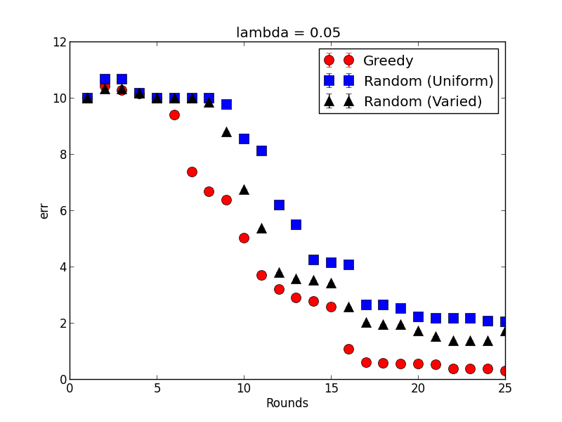
In Figure 4(a), we display our main experimental results for four different algorithms in the policy observation setting, and in Figure 4(b) for the trajectory setting. Error represents , where is an algorithm’s prediction, with error bars representing standard error over simulations.
In Figure 4(a), the horizontal line displays the best results we achieved without repeated experimentation. If the learner only selects a single environment , observing policy , it is stuck with whatever experimental unidentifiability exists in . In such a scenario, we can select a according to a classic IRL heuristic, given by LP (1) in Section 5.1, for some choice of in LP (1). Since the performance of this method depends both on which environment is used, and the choice of , we randomly generated different environments, and for each of those environments selected . We then evaluated each of these single-environment approaches with simulations, the best error among these different single-environment algorithms is displayed by the horizontal line. Immediately we see that the experimental unidentifiability from using a single environment makes it difficult to distinguish the actual reward function, with for the best choice of and greater than .
The remaining algorithms — which we will describe in greater detail below — conduct repeated experimentation. Each of these algorithms uses a different rule to select a new environment on each round. Given the sequence of (environment, policy) pairs generated by each of these algorithms, we solve the LP (2) on at the end of each round. This is done with the same choice of for each of the algorithms.
Besides the algorithm of the previous section, we implement two other algorithms, which conduct repeated experiments, but do so non-adaptively. , in each round, selects a maze uniformly at random from the space of possible mazes (each wall is present with probability ). Note that will tend to select mazes where roughly half of the walls are present. Thus, we also consider which, in each round, selects a maze from a different distribution . Mazes drawn from are generated by a two-step process. First, for each row and column , we select numbers i.i.d. from the uniform distribution on . Then each wall along row (column respectively) is created with probability ( respectively). Although the probability any particular wall is present is still , the correlations in creates more variable mazes (e.g. allowing an entire row to be sparsely populated with walls).
We implement Algorithm 1, , of the previous section, by approximating the maximization in Line 5 in Algorithm 1. This approximation is done by sampling environments from , the same distribution used by . In the policy observation setting, samples are first drawn from the consistent set using a hit-and-run sampler (9), which is an MCMC method for uniformly sampling high-dimensional convex sets in polynomial time. These same samples are also used to estimate the volume . In the trajectory setting, we first sample trajectories on an environment , then we use for an arbitrary , as a proxy for .
Examining the results, we see that converges significantly quicker than either of the non-adaptive approaches. After rounds of experimentation in the policy observation setting, attains error , while the best non-adaptive approach attains . only requires rounds to reach a similar error of . We note further that the performance of seems to continue to improve, while the non-adaptive approaches appear to stagnate. This could be due to the fact that after a certain number of rounds, the non-adaptive approaches have received all the information available from the environments typically sampled from their distributions. In order to make progress they must receive new information, in contrast to , which is designed to actively select the environments that will do just that.
Finally, runs by selecting a sequence of environments, resulting in observations . It then selects from using LP (2). Thus, the regularization parameter in LP (2) is a free parameter for that we took to be equal to for results (Figure 4(a)). We conclude by experimentally analyzing the sensitivity of to the choice of this parameter, as well as of , and , which also select according to LP (2). As is increased, eventually the LP over-regularizes, and is optimized taking . In our setting, once this begins to occur, and we begin to see pathological behavior (Figure 5(a)). This problem occurs in standard IRL, and one approach ((10)) is to select a large lambda before this transition, hence our choice of . However, even for significantly smaller , the results are qualitatively similar (Figure 5(b)) to those in Figure 4(a). We find that as long as is not too large, the results are not sensitive to the choice of .

7. Conclusions
We provide a number of contributions in this work. First, we separate the causes of unidentifiability in IRL problems into two classes: representational, and experimental. We argue that representational unidentifiability is superficial, leading us to redefine the problem of identification in IRL according to Definition 2. While previous work does not distinguish between these two classes, we demonstrate that, by doing so, algorithms can be designed to eliminate experimental unidentifiability while providing formal guarantees.
Along the way, we derive a new model for IRL where the learner can observe behavior in multiple environments, a model which we believe is interesting in its own right, but also is key to eliminating experimental unidentifiability. We give an algorithm for a very powerful learner who can observe agent behavior in any environment, and show that the algorithm -identifies an agent reward defined on states, while observing behavior on only environments. We then weaken this learner to model more realistic settings where the learner might be restricted in the types of environments it may choose, and where it may only be able to elicit a small number of demonstrations from the agent. We derive a simple adaptive greedy algorithm which will select a nearly optimal (with respect to reducing the volume of possible reward function) set of environments. The value of the solution found by this greedy algorithm will be a comparable to the optimal algorithm which uses a logarithmic factor fewer number of experiments.
Finally, we implement the algorithm in a simple maze environment that nevertheless demonstrates the value of eliminating experimental unidentifiability, significantly outperforming methods that attempt to perform IRL from a single environment.
References
- [1] P. Abbeel, A. Coates, M. Quigley, and A. Y. Ng. An application of reinforcement learning to aerobatic helicopter flight. Advances in neural information processing systems, 19:1, 2007.
- [2] P. Abbeel and A. Y. Ng. Apprenticeship learning via inverse reinforcement learning. In Proceedings of the twenty-first international conference on Machine learning, page 1. ACM, 2004.
- [3] U. Chajewska, D. Koller, and R. Parr. Making rational decisions using adaptive utility elicitation. In AAAI/IAAI, pages 363–369, 2000.
- [4] A. Coates, P. Abbeel, and A. Y. Ng. Learning for control from multiple demonstrations. In Proceedings of the 25th international conference on Machine learning, pages 144–151. ACM, 2008.
- [5] A. Coates, P. Abbeel, and A. Y. Ng. Apprenticeship learning for helicopter control. Communications of the ACM, 52(7):97–105, 2009.
- [6] D. Golovin and A. Krause. Adaptive submodularity: A new approach to active learning and stochastic optimization. In COLT, pages 333–345, 2010.
- [7] A. Guillory and J. Bilmes. Interactive submodular set cover. In Proceedings of the International Conference on Machine Learning, 2010.
- [8] M. Lopes, F. Melo, and L. Montesano. Active learning for reward estimation in inverse reinforcement learning. In Machine Learning and Knowledge Discovery in Databases, pages 31–46. Springer, 2009.
- [9] L. Lovász. Hit-and-run mixes fast. Mathematical Programming, 86(3):443–461, 1999.
- [10] A. Y. Ng and S. J. Russell. Algorithms for inverse reinforcement learning. In Icml, pages 663–670, 2000.
- [11] D. Ramachandran and E. Amir. Bayesian inverse reinforcement learning. Urbana, 51:61801, 2007.
- [12] N. D. Ratliff, J. A. Bagnell, and M. A. Zinkevich. Maximum margin planning. In Proceedings of the 23rd International Conference on Machine Learning, pages 729–736. ACM, 2006.
- [13] K. Regan and C. Boutilier. Regret-based reward elicitation for markov decision processes. In Proceedings of the Twenty-Fifth Conference on Uncertainty in Artificial Intelligence, pages 444–451. AUAI Press, 2009.
- [14] K. Regan and C. Boutilier. Robust policy computation in reward-uncertain mdps using nondominated policies. In AAAI, 2010.
- [15] K. Regan and C. Boutilier. Eliciting additive reward functions for markov decision processes. In IJCAI Proceedings-International Joint Conference on Artificial Intelligence, volume 22, page 2159, 2011.
- [16] C. A. Rothkopf and C. Dimitrakakis. Preference elicitation and inverse reinforcement learning. In Machine Learning and Knowledge Discovery in Databases, pages 34–48. Springer, 2011.
- [17] W. D. Smart and L. P. Kaelbling. Effective reinforcement learning for mobile robots. In Robotics and Automation, 2002. Proceedings. ICRA’02. IEEE International Conference on, volume 4, pages 3404–3410. IEEE, 2002.
- [18] U. Syed and R. E. Schapire. A game-theoretic approach to apprenticeship learning. In Advances in neural information processing systems, pages 1449–1456, 2007.
- [19] J. Von Neumann and O. Morgenstern. Theory of games and economic behavior (60th Anniversary Commemorative Edition). Princeton university press, 2007.
- [20] B. D. Ziebart, A. L. Maas, J. A. Bagnell, and A. K. Dey. Maximum entropy inverse reinforcement learning. In AAAI, pages 1433–1438, 2008.
Appendix A Proof of Theorem 3
Theorem 6.
For any , if and only if they have the same canonicalized representation.
Proof.
By definition, the canonicalized representation of any reward function is attained by scaling and translation. Therefore, by Theorem 2, if and are both canonicalized as , we have that and , and therefore .
In the other direction, suppose and are canonicalized to and respectively, where . Again, by Theorem 2, we have that and . Thus, to prove the theorem, it is sufficient to argue that and are not behaviorally equivalent.
If one of is and the other is not, then it is straightforward to show that they are not behaviorally equivalent. Thus, we focus on the case where both and are not . We consider three cases.
First, suppose that because they have different minimally-rewarding states. Without loss of generality suppose that there is some with but . Furthermore, let be any state such that . Consider an environment with two actions and . Action deterministically transitions to state from any other state, while action determininstically transitions to state from any other state. Let be the policy that always takes action . . However, if , this means that , and therefore all policies are in . Thus, , and are not behaviorally equivalent.
Next, suppose that because they have different maximally-rewarding states. Analagously to the previous case, suppose without loss of generality there is some with by , and let be any state such that (which exists since ). Define the environment in the same way as the previous case. This time, , while .
Finally, suppose that and share the same maximally and minimally rewarding states, but there exists some such that . Let be any state such that and let be any state such that . Without loss of generality suppose that . Let be the environment with two actions and . Let be any real number . From every state, action transitions to state with probabiity and to state with the remaining probability. From every state action transtions to state deterministically. The reward for taking action in any state under either reward function is , while action gives a reward of under and under . Thus, , concluding the proof. ∎
Appendix B Proof of Greedy’s Performance
Given a set and component , we use to denote the union of the singleton set with . We begin by redefining:
where is an upper bound .
Let be the set of possible observations, so that is a trajectory in the trajectory setting, and a policy in the policy setting. Let be the space of possible environments. WWe first establish that is indeed submodular.
Lemma 2.
is a submodular, non-decreasing function on .
Proof.
Fix any , and . By definition of , we have that and , and so:
This establishes submodularity of . Since is arbitrary and the right-hand-side of the second equality is non-zero, is also monotone. ∎
Let denote the set of functions mapping environments to observations. For any and , overload , so that .
Now suppose that environments where labeled according to some , and consider an algorithm which knowing , selects the fewest number of environments , so that . Given such an algorithm, we can now define the General Identification Cost, which identifies the worst-possible labelling strategy in . In particular:
Recall the definition from the main body:
This is the largest that an algorithm can guarantee to make with environments, when environments are consistently labeled by some . Let be the algorithm satisfying the .
Lemma 3.
Proof.
Fix any . Consider two cases. First suppose that there exists some such that , but is inconsistent with the labeling of any . By defintion of , , and since , the Lemma is proven.
Otherwise, it must be that all , , is consistent with the labeling of some . By definition of , running against the labels provided by is guaranteed to result in a sequence of environments , , satisfying . is a witness that is at most . ∎
Given an environment and true reward , let denote the set of possible observations (in either the policy or trajectory setting).
Lemma 4.
For any , such that , there exists an environment such that:
Proof.
Suppose not. Then for every environment , there exists some and such that:
Now let be defined so that:
| (3) | ||||
| (4) |
By definition of , we have that:
So there exists a set of environments , with , such that , and by monotonicity of , we know that . Let .
However, despite , repeatedly applying the submodularity of , then applying equation (4) implies:
This establishes a contradiction. ∎
We can now prove the main theorem:
Theorem 7.
returned by the Greedy Environment Selection algorithm satisfies when .
Proof.
Let denote the subsequence consisting of the first environment, observation pairs. If for some , , then there is nothing to prove. Otherwise, by applying Lemma 3, and the definition of the algorithm, we know that:
which implies:
Using the fact , we can conclude:
Applying Lemma 4 and substituting completes the proof.
∎