Efficiency and Optimality of Largest Deficit First Prioritization: Resource Allocation for Real-Time Applications

We consider an abstract system that serves $n$ users indexed from $1$ to $n$. Let $N=\{1,2,\cdots,n\}$ be the user set. The system operates in discrete time, over periods $t=1,2,\cdots$. In each period, it picks a user priority decision $\mathbf{d}=(d_{1},d_{2},\dots,d_{n})$ where $d_{m}$ is the index of the user with $m^{\text{th}}$ highest priority. We let $D$ denote the set of all possible priority decisions and let $|D|$ represent the number of possible decisions, thus, $|D|=n!$

In each period, given the priority decision $\mathbf{d}$ passed to the underlying resources, since there are intrinsic uncertainties in users’ workloads, each user $i$ achieves a non-negative random QoS payoff, denoted by $V_{i}(\mathbf{d})$. We let $\mathbf{V}(\mathbf{d})=(V_{1}(\mathbf{d}),V_{2}(\mathbf{d}),\cdots,V_{n}(\mathbf{d}))$. We assume the payoffs are independent across periods. The distribution of $\mathbf{V}(\mathbf{d})$ depends on the selected priority decision $\mathbf{d}$ and the expected payoff vector given $\mathbf{d}\in D$ is denoted by $\mathbf{p}(\mathbf{d})=\expectation[\mathbf{V}(\mathbf{d})]$. We assume all possible payoff vectors form a finite rational set. Moreover, we naturally assume that for each user $i\in N$, there exists a decision $\mathbf{d}$ such that $p_{i}(\mathbf{d})>0$.

Each user requires a long-term average QoS payoff $q_{i}\geq 0$ as the QoS requirement. We let $\mathbf{q}=(q_{1},q_{2},\cdots,q_{n})$ and assume $q_{i}$’s are rational¹¹ 1 All the results in this paper can be generalized to models with irrational values. For simplicity in the proof we do not consider that level of generality. . We denote by $\mathbf{d}(t)$ the priority decision at period $t$. To keep track of the deficits between required and achieved QoS payoffs, for each user $i\in N$ and period $t+1$, we define²² 2 We truncate the deficit at $0$ for the convenience of defining feasibility in the sequel. Removing the truncation won’t change the results in the paper.

where $[x]^{+}=\max[x,0]$.

The goal is thus to devise user prioritization policies which will meet users’ long-term payoff requirements.

The process $\{\mathbf{X}(t)\}_{t\geq 1}$ is a Markov chain under any such policy. We assume the initial state $\mathbf{X}(0)$, the requirements $\mathbf{q}$, the set of all possible payoff vectors and the user prioritization policy make $\{\mathbf{X}(t)\}_{t\geq 1}$ an irreducible Markov chain.

The expected payoff vectors $P=\{\mathbf{p}(\mathbf{d})|\mathbf{d}\in D\}$ could in principle be statistically inferred from the history events or by repeated experiments. However, in a practical setting this can be challenging and it is of interest to find a policy that performs well and uses little a-priori information regarding the exponential set of expected payoff vectors $P$.

Note that this model is general in the sense that the “impact” of priority decisions $\mathbf{d}\in D$ on the QoS payoff vectors $P$ is at this point general, whereas the specific resource and workload models in prior work, e.g., [7, 16, 17], implicitly impose properties on $P$ and therefore restrict the results significantly.

Our model can for example capture a centralized computing infrastructure supporting Soft Real-Time (SRT) applications where the $n$ users share compute resources. In a cloud-based collaborative video conferencing context, a user might correspond to an individual end user and the period length might correspond to the length of a group of video frames.

The users generate streams of tasks periodically. Specifically in each period a user generates several tasks. A task may further consist of a graph of possibly dependent sub-tasks with (possibly) random processing requirements, i.e., workloads. These tasks/sub-tasks need to be fully completed before the end of the period. For real-time services, it is generally useless to process a task after its deadline. For example, in the video conferencing context it is not desirable to present an out-of-date frame. Therefore, we assume tasks/sub-tasks not completed on time are dropped.

In each period $t$, the user prioritization policy picks a user priority decision $\mathbf{d}(t)$, based on which compute resources are allocated to process tasks. Given the task processing results, a payoff $V_{i}(\mathbf{d}(t))$ is achieved for each user $i$ based on whether the tasks were successfully processed, or how much of the task graphs were completed. In general, $V_{i}(\mathbf{d}(t))$ may represent any user-specific QoS payoff per period, that can be averaged over time, e.g., the quality/resolution of video frame processing, or the number of task completions. Accordingly the vector $\mathbf{q}$ represents the long-term average QoS requirements.

As indicated in the introduction, our model also applies to a complex network of heterogeneous compute and communication resources, as long as users periodically and synchronously generate tasks that require timely processing on diverse resources and moving around in the network, e.g., as shown in Figure 1.

Given the priority decision in each period, the network of resources coordinate according to some priority-based resource allocation mechanism to accelerate the processing of tasks with high priorities, by reducing the communication/queueing delays, processing with higher processor speed, allocating more shared resources, etc.

Again, different users can define their payoffs in different ways and specify their QoS requirements accordingly.

The set of all feasible long-term payoff requirement vectors will be referred to as the system feasibility region $F$. We let $F_{\eta}$ denote the feasibility region of a user prioritization policy $\eta$. To characterize $F$ we introduce some further notation.

A vector $\mathbf{x}$ is said to be dominated by a vector $\mathbf{y}$ if $x_{i}\leq y_{i}$ for all $i$ and is denoted by $\mathbf{x}\preceq\mathbf{y}$. We define $\mathbf{x}\prec\mathbf{y}$, $\mathbf{x}\succeq\mathbf{y}$ and $\mathbf{x}\succ\mathbf{y}$ in a similar manner.

Given the set of priority decisions $D$ and the expected payoff vectors $P=\{\mathbf{p}(\mathbf{d})|\mathbf{d}\in D\}$, we let $C$ be the set of requirement vectors $\mathbf{q}\in\mathbb{R}^{n}_{+}$ which are dominated by a vector in the convex hull of $P$ denoted Conv($P$), i.e.,

Figure 2 exhibits $C$ for a two-user (left figure) and three-user (right figure) setting. In the two-user setting, the points labeled $\mathbf{p}(\mathbf{d}_{1})$ and $\mathbf{p}(\mathbf{d}_{2})$ are the expected payoff vectors of two priority decisions, i.e., where User 1 or User 2 has higher priority, respectively. The shadowed area represents $C$. In the three-user setting, the circles represent the $6$ possible expected payoff vectors, and the region dominated by their convex hull is $C$. Note that in a $n$-user scenario where $n\geq 3$, as displayed the expected payoff vectors need not be on a hyperplane in the $n$-dimensional space. As we will see this is essentially the source of complexity in studying such systems.

Clearly, for any requirement vector $\mathbf{q}$ in the interior of $C$, denoted by $\text{int}(C)$, one can achieve $\mathbf{q}$ if one is allowed to do probabilistic time sharing among priority decisions by picking decisions according to a pre-computed probability distribution whose mean payoff dominates $\mathbf{q}$. Therefore, $\text{int}(C)\subseteq F$. We can also show the following result.

Intuitively, if $\mathbf{q}$ is feasible, it is fulfilled by some user prioritization policy that in the long-term picks each priority decision some fraction of the time and thus, $\mathbf{q}$ is dominated by some point in the convex hull of $P$. This is similar to prior work, e.g., [27]. See the appendix for a detailed proof. In other words, $C$ is different from $F$ by at most a boundary, and therefore, characterizes $F$ for practical purposes. Thus, in the sequel we will also refer to $C$ as the system feasibility region.

Ideally, it is desirable to devise an “optimal” policy that can fulfill all feasible requirements. More formally, a user prioritization policy $\eta$ is said to be feasibility optimal if $\text{int}(C)\subseteq F_{\eta}\subseteq\text{cl}(C)$. Similar to prior work [27, 28], the following max weight-like policy is one such feasibility optimal policy.

However, the MW policy and time sharing policies require full knowledge of $P$ which is challenging in complex practical systems. Moreover, these policies are hard to implement since they involve solving fairly complex optimization problems, i.e., Eq (3). Changes in the user set or payoff requirement vector $\mathbf{q}$ will also impact the realization of these policies. In summary, the requirements in terms of a-priori knowledge, the computational complexity and lack of flexibility to changes make them hard to use in practice. This motivates the policies considered in the next subsection.

For ease of reference, Table 3.1 provides a summary of the notation used to denote various regions used in the rest of the paper—some of these are introduced in the sequel.

The LDF user prioritization policies require no a-priori knowledge of the system, are simple to implement and adapt easily to changes in $\mathbf{q}$ or the user set. In particular we shall characterize the feasibility regions of these policies by providing an inner bound.

Clearly, the $\mathbf{w}$-LDF prioritization policies do not require knowledge of the expected payoff vectors $P$. Note that we still use deficit feedback to stabilize the system. In terms of computational complexity, solving (3) is $O(n!)$ while sorting weighted deficits only requires $O(n\log n)$. It also allows us to further differentiate the performance across users by assigning different weights. The impact of weights is discussed in Section 6.

Prior work has established that the LDF policy need not be feasibility optimal. Therefore, a key question is whether the feasibility regions for the $\mathbf{w}$-LDF policies are acceptable and to characterize the gap between their feasibility regions and the system feasibility region $F$. To that end, we first provide an inner bound, denoted by $R_{\text{IB}}$, for the feasibility region of any $\mathbf{w}$-LDF policy.

In other words, if $\mathbf{q}\in R_{\text{IB}}$, it is feasible under all $\mathbf{w}$-LDF policies except perhaps boundary points. The underlying intuition for this bound is as follows. A vector $\mathbf{q}$ is in $R_{\text{IB}}$ if there is a weight vector $\boldsymbol{\alpha}\succ\mathbf{0}$ such that for any subset of users $S$, and decisions giving users in $S$ the highest priorities, the weighted sum of payoff requirement $\sum\limits_{i\in S}\alpha_{i}q_{i}$ will not exceed the least sum weighted payoff $\sum\limits_{i\in S}{\alpha}_{i}p_{i}(\mathbf{d})$. Based on $\boldsymbol{\alpha}$, we can construct an appropriate Lyapunov function to show feasibility for $\mathbf{q}$ and each $\mathbf{w}$. See Appendix 8.3 for the proof.

Understanding the geometry of $R_{\text{IB}}$ enables us to characterize the performance gap between $\mathbf{w}$-LDF and feasibility optimal policies. Let us informally consider the geometry of $R_{\text{IB}}$ for the two special cases in Figure 2. In the two-user case in Figure 2, $R_{\text{IB}}$ is the same as $C$ and thus, the $\mathbf{w}$-LDF policies are feasibility optimal. However, in the three-user case in Figure 2, this need not be true. Indeed, in this setting, the region $R_{\text{IB}}$ corresponds to $C$ minus the convex hull of $P$, modulo some boundary points. This is exhibited in Figure 3. In the next subsection, we will formalize these observations and show under what conditions they hold true.

In order to formally characterize the geometry of $R_{\text{IB}}$ we will add a further natural requirement to the general model.

We define $S_{i}(\mathbf{d})$ to be the set of users that have higher priorities than user $i$ under decision $\mathbf{d}$.

In other words, a user $i$ can expect to get a higher payoff if some users with higher priority are re-assigned lower priorities. This property characterizes in a broad sense how priorities impact the expected payoffs when the underlying system allocates resources. It is a natural condition but need not hold in general.

We shall define $B$ to be the set of payoff requirement vectors $\mathbf{q}$ which dominate a vector in the convex hull of $P$, i.e.,

We call $B$ the dominant of the convex hull. Contrast this to the definition of $C$ in (2).

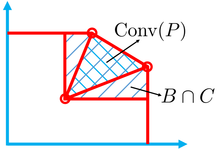
For the special cases in Figure 2 and 3, $B\cap C$ equals to $\text{Conv}(P)$, but in general it can be larger than $\text{Conv}(P)$. Figure 4 shows a conceptual picture of what could happen. The three circles represent three possible expected payoff vectors. Here, the whole shadowed area $B\cap C$ is larger than the region Conv$(P)$ which is the triangle formed by the three circles. Note that this is only a conceptual example to help visualize $B\cap C$ in higher dimensions. In reality for two dimensions, i.e., systems with two users, we know there are only $2$ expected payoff vectors as shown in Figure 2.

In the sequel we will see that given monotonicity in payoffs, $R_{\text{IB}}$ is obtained by “removing” $B\cap C$, rather than just $\text{Conv}(P)$ from $C$. To develop this result we need some further notation associated with each subset of users $S\subseteq\{1,2,\cdots,n\}$.

The projection of a vector $\mathbf{x}$ on the subspace of $S$ is denoted by $\mathbf{x}^{S}$, i.e.,

We let $P^{S}\equiv\{\mathbf{p}^{S}(\mathbf{d})|\mathbf{d}\in D(S)\}$ represent the projections of expected payoff vectors corresponding to decisions in $D(S)$, i.e., which assign the highest priorities to users in $S$.

Given a subset $S$ and $P^{S}$, we define the feasibility region $C^{S}$ and the dominant of the convex hull $B^{S}$ as follows.

Note that $C^{S}$ and $B^{S}$ are not necessarily the same as projecting $C$ and $B$ on the subspace of $S$, respectively. This is because in the definitions of $C^{S}$ and $B^{S}$, we only focus on a subset of decisions $D(S)$ rather that the full decision set $D$.

Let us now define a region $R$ which will help characterize the geometry of the inner bound $R_{\text{IB}}$.

One can visualize obtaining the set $R$ as a process of removing $B^{S}\cap C^{S}$ from $C^{S}$ in all subspaces corresponding to all subsets $S$. The geometry of $R_{\text{IB}}$ is then captured as follows.

By Theorem 3.5 and Theorem 3.8, we immediately get

Since $R$ is obtained by removing $B^{S}\cap C^{S}$ from $C^{S}$ for each $S$, if what is removed is nothing more than a boundary, the difference between $R$ and $C$ is at most a boundary and thus $\mathbf{w}$-LDF policies are feasibility optimal. It is easy to see this happens when vectors in $P^{S}$ lie on a hyperplane for each subset of users $S$. This can be formalized as follows.

The conditions for this theorem are akin but not equivalent to the conditions introduced in [7] for the generalized switch model. Specifically, we require the system to satisfy monotonicity in payoffs and subset payoff equivalence. The work in [7] requires local pooling in the generalized switch model. In the model in [7], given a priority decision $\mathbf{d}=(d_{1},d_{2},\cdots,d_{n})$ where $d_{i}$ is the index of the queue with the the $i^{\text{th}}$ highest priority, the queue service rate vector can be denoted by $\mathbf{m}(\mathbf{d})$, where $m_{d_{i}}(\mathbf{d})$ represents the units of work that can be removed from queue $d_{i}$ in one time slot under priority decision $\mathbf{d}$. $\mathbf{m}(\mathbf{d})$ is akin to $\mathbf{p}(\mathbf{d})$ in our context. However, the generalized switch model in [7] implies properties on the service rate vectors $\mathbf{m}(\mathbf{d})$. For example, it implies that for all $\mathbf{d}=(d_{1},d_{2},\cdots,d_{n})$, we have $m_{d_{1}}(\mathbf{d})\geq m_{d_{1}}(\mathbf{d}^{\prime})$ for all $\mathbf{d}^{\prime}$, and $m_{d_{2}}(\mathbf{d})\geq m_{d_{2}}(\mathbf{d}^{\prime})$ for all $\mathbf{d}^{\prime}$ satisfying $m_{d_{1}}(\mathbf{d})=m_{d_{1}}(\mathbf{d}^{\prime})$, etc. These implicit requirements do not necessarily hold in systems which satisfy the conditions in Theorem 3.10.

If the system has only two users, then clearly subset payoff equivalence is satisfied since the two expected payoff vectors are always on a line. Therefore, we get the following corollary.

Note that in a two-user scenario, the property of monotonicity in payoffs simply means a user gets higher payoff under the higher priority than its payoff under the lower priority. In Section 4.2 we will consider systems serving two classes of exchangeable users and use this corollary to show the optimality of LDF-like policies.

When the conditions in Theorem 3.10 do not hold, one can still study the efficiency ratio, see e.g., [16], to evaluate the performance of $\mathbf{w}$-LDF policies.

Clearly $\gamma_{\mathbf{w}\text{-LDF}}$ equals to $1$ if and only if the $\mathbf{w}$-LDF policy is feasibility optimal.

If a system does not satisfy subset payoff equivalence, i.e., for some subset of users $S$ the vectors in $P^{S}$ are not on the same hyperplane, we can characterize the “heterogeneity” of these vectors based on the following notion.

The optimal $\boldsymbol{\alpha}^{S}$ is such that the projections of the vectors in $P^{S}$ on $\boldsymbol{\alpha}^{S}$ are as close to each other as possible.

Clearly if the vectors in $P^{S}$ are on the same hyperplane, then $\sigma_{S}=1$ and the optimal $\boldsymbol{\alpha}^{S}$ is the normal vector to the hyperplane. Intuitively, $\sigma_{S}$ characterizes the degree to which the vectors in $P^{S}$ deviate from being on the same hyperplane.

This notion enables us to characterize the efficiency ratio of $\mathbf{w}$-LDF for a given system.

Note that by picking any $\boldsymbol{\alpha}\succ\mathbf{0}$, we can get lower bounds on $\sigma_{S}$ for all subsets $S\subseteq N$ by placing its projection $\boldsymbol{\alpha}^{S}$ into (6). Thus, any $\boldsymbol{\alpha}\succ\mathbf{0}$ enables us to construct a lower bound on $\gamma_{\mathbf{w}\text{-LDF}}$. A trivial option is $\boldsymbol{\alpha}=\mathbf{1}$, where for each subset $S$ the value of $\langle\mathbf{1}^{S},\mathbf{p}^{S}(\mathbf{d})\rangle$ represents the sum payoff of users in $S$ under decision $\mathbf{d}$.

We have shown that the efficiency and optimality of the $\mathbf{w}$-LDF policies is related to $R_{\text{IB}}$. Understanding and analyzing the geometry of $R_{\text{IB}}$ can in principle enable us to provide feedback to the designers of priority-based resource allocation mechanisms regarding which specific priority decision or set of priority decisions are problematic and bottlenecks for the system so that the designers can focus on improving the resource allocation for these problematic decisions. For example, in the conceptual setting shown in Figure 4, the priority decision corresponding to the lower left circle is the “bottleneck” of the system and should be targeted to make the dominant of the convex hull as small as possible. This is of particular interest for some practical systems where it is possible to get explicit knowledge of $P$ which reflect the underlying priority-based resource allocation, e.g., by collecting data over a long time.

A priority decision is problematic if the associated underlying resource allocation suffers from resource contention, blocking among users/applications, or even deadlocks on compute resources, etc. Based on feedback regarding the bottlenecks, the designer could improve the associated resource allocation schemes, e.g., by increasing the processing speed of the certain computing resources, spending more energy, reducing the contention, and/or resolving the blocking/deadlock, and thus, improve the efficiency of the overall system under the $\mathbf{w}$-LDF prioritization policies.

We shall start by showing that for systems that are “symmetric”, $\mathbf{w}$-LDF policies are feasibility optimal.

In other words, exchanging the priorities of two users in $S$ will simply exchange their expected payoffs without impacting that of other users. This would be true if the priority-based resource allocation were symmetric for users in $S$ and the users generate tasks with identically distributed or exchangeable workloads.

If the users in $N$ have exchangeable expected payoffs, we can verify the property of subset payoff equivalence by picking $\boldsymbol{\alpha}^{S}=\mathbf{1}^{S}$ for each subset of users $S$. Therefore, by Theorem 3.10 we get the following corollary.

In this subsection, we first consider a system supporting two classes of exchangeable users. Formally, a class of users is exchangeable if they have exchangeable expected payoffs and the same QoS requirement. The users in different classes may have distinct payoffs and QoS requirements. In some contexts it is of practical interest to first prioritize the classes and then prioritize users in each class, respectively. We refer to such schemes as using class-based hierarchical prioritization.

In practice, depending on whether the priorities of classes can change dynamically, there are two types of class-based hierarchical prioritization: Type $1$ where the class priorities are fixed, and Type $2$ where one can dynamically prioritize classes of users, and then users within each class.

The first type of hierarchical prioritization might correspond to a setting where the users/applications are separated into human-interactive/high-QoS and background-processing/low-QoS categories [11], and it is always desirable to first process high-QoS users. In this setting, the problem is reduced to a collection of independent user prioritization problems similar to the one considered in this paper. By Corollary 4.2, $\mathbf{w}$-LDF is feasibility optimal to prioritize users in each class.

The second type of dynamic hierarchical prioritization might be of interest in systems where switching between processing different user classes involves overheads, and/or where it is inefficient to mix the processing of different user classes, probably because of resource contention or deadlocks.

In this setting, we propose a class-based hierarchical-LDF policy that in each period works in two steps by (1) prioritizing classes by LDF based on the aggregate deficits, i.e., the sum of deficits for users in the same class, and (2) prioritizing users in each class according to LDF based on individual users’ deficits. The framework of hierarchical-LDF is exhibited in Figure 5. Note that here LDF can be replaced by $\mathbf{w}$-LDF for any $\mathbf{w}\succ\mathbf{0}$ and the following result would hold.

The proof follows directly from Corollary 3.11 and 4.2. By Corollary 3.11 we know the class-based LDF policy is optimal to set priorities amongst the two classes and by Corollary 4.2 we know the LDF-based user prioritization is also optimal for the exchangeable users in each class.

More generally, for systems serving multiple (more than two) classes of exchangeable users, one can view each class as a “super user”, and define the aggregate payoff and QoS requirement for a super user to be the sum of payoffs and QoS requirements for users in that class, respectively. Then the dynamic prioritization of super users can be viewed as the problem considered in this paper. Therefore, by Theorem 3.10, if the system with the super users’ expected aggregate payoffs satisfies monotonicity in payoffs and subset payoff equivalence, the LDF policy is a feasibility optimal choice for prioritizing super users and thus, the hierarchical-LDF policy is feasibility optimal among all class-based hierarchical prioritization policies. Indeed, all the results we have introduced, e.g., Theorem 3.3-3.14, still hold for the prioritization of these super users.

In Table 6.1 we consider a requirement vector $\mathbf{q}$ that is feasible under the $\mathbf{w}$-LDF policies and display the achieved $\mathbf{p}$ under two different weight vectors $\mathbf{w}$. For each weight vector $\mathbf{w}$, we verify that $w_{i}(p_{i}-q_{i})$ is the same for all three users. Contrasting the two lines in Table 6.1, we can see that for a system which can deliver more than required, changing the weight vector reallocates the excess payoffs and gives more excess payoffs to users with smaller weights.

If a user’s task is not completed in a period, we call it a failure event. The requirement vector $\mathbf{q}$ focuses on long-term task completion ratio, but it would likely be undesirable for a user to experience consecutive or clustered failure events. Figure 6 gives an example of failure events. In this subsection we consider the same $\mathbf{q}=(0.8,0.6,0.4)$ used above and explore the clustering of failures under two $\mathbf{w}$-LDF policies.

We consider Inter-Failure Intervals (IFIs) between typical failures. IFI is supported on the set $\{1,2,3,\cdots\}$. To quantitatively evaluate the clustering of the failures, we focus on the standard deviation (SD) of the IFIs for each user. One extreme case is that failures happen strictly periodically and therefore, the SD is $0$. Intuitively, a user with a smaller IFI SD implies that the user experiences less clustered failures.

Next we introduce an evaluation benchmark. For each user $i$, we know $1-p_{i}$ represents the time-averaged failure ratio. If the failure happens in each period independently with probability $1-p_{i}$, the IFI can be modeled by a geometric random variable supported on the set $\{1,2,3,\cdots\}$ with the parameter being $1-p_{i}$. We use the SD of such a geometric random variable as a benchmark.

Under some $\mathbf{w}$-LDF policy, we define SD ratio of user $i$ to be the ratio of user $i$’s IFI SD to the SD of the geometric random variable with parameter $1-p_{i}$. Table 6.2 shows the SD ratios of three users under two different weight vectors $\mathbf{w}$. Under $\mathbf{w}=(1,1,1)$, the ratios are less than $1$, indicating that the failures under the LDF policy are less clustered compared to the scheme where failure event happens i.i.d. in each period. The last two columns in Table 6.2 indicates that increasing the weight of user $i$ reduces the degree of failure clustering for user $i$ but at the price of other users’ more clustered failures. Thus, the users’ sensitivities to clustered failures is another factor to consider when one assigns weights to users.

Given $\mathbf{q}\in F$, since it is feasible there exists a user prioritization policy $\eta$ that fulfills $\mathbf{q}$, i.e., the Markov chain $\{\mathbf{X}(t)\}_{t\geq 1}$ is positive recurrent, which implies there exists a stationary distribution over the state space. Since $\eta$ is a stationary policy that picks $\mathbf{d}(t+1)$ based on $\mathbf{X}(t)$, by Ergodic Theorem each priority decision $\mathbf{d}$ is selected with some time fraction $\alpha_{\mathbf{d}}$ such that $\sum\limits_{\mathbf{d}\in D}\alpha_{\mathbf{d}}=1$ . If we consider $X_{i}(t)$ as a queue, the average arrival $q_{i}$ should not be bigger than the average departure which is given by $\sum\limits_{\mathbf{d}\in D}\alpha_{\mathbf{d}}p_{i}(\mathbf{d})$ since otherwise $X_{i}(t)$ goes a.s. to infinity and the chain cannot be positive recurrent.

Therefore,

which implies $\mathbf{q}\in C\subseteq\text{cl}(C)$.

We start by introducing a lemma.

To understand this lemma, since any vector in $C$ is dominated by some $\mathbf{q}\in\text{Conv}(P)$, we consider for simplicity a $\mathbf{q}\in\text{Conv}(P)$. Such a vector can be expressed as a convex combination of expected payoff vectors, i.e., $\mathbf{q}=\sum\limits_{\mathbf{d}\in D}\alpha_{\mathbf{d}}\mathbf{p}(\mathbf{d})$, where $\sum\limits_{\mathbf{d}\in D}\alpha_{\mathbf{d}}=1$ and $\alpha_{\mathbf{d}}\geq 0,\forall\mathbf{d}\in D.$

Now we have

This actually proves the necessity of the condition. The formal proof is shown below.

We first introduce some further notation. Given two vectors $\boldsymbol{a}=(a_{1},a_{2},\cdots,a_{n})$ and $\mathbf{b}=(b_{1},b_{2},\cdots,b_{n})$, we denote by $\boldsymbol{a}\circ\mathbf{b}=(a_{1}b_{1},a_{2}b_{2},\cdots,a_{n}b_{n})$ the entrywise product.

For any $\mathbf{w}\succ\mathbf{0}$ and $\mathbf{q}\in\text{int}(R_{\text{IB}})$, the goal is to show that $\mathbf{q}$ can be fulfilled by the $\mathbf{w}$-LDF policy.

Let $\boldsymbol{\beta}=(\frac{1}{w_{1}},\frac{1}{w_{2}},\cdots,\frac{1}{w_{n}})$. By definition of interior there exists an $\epsilon>0$ such that ${\mathbf{q}}^{\prime}=\mathbf{q}+\epsilon\boldsymbol{\beta}\in R_{\text{IB}}$. By definition of $R_{\text{IB}}$, there exists a vector $\boldsymbol{\alpha}\succ\mathbf{0}$ such that $\mathbf{q}^{\prime}$ and $\boldsymbol{\alpha}$ satisfy the conditions (4).

Consider the following candidate Lyapunov function:

Note that we consider a process $\{\mathbf{X}(t)\}_{t\geq 1}$ that is driven by the $\mathbf{w}$-LDF policy. In period $t+1$, by similar analysis as in (13) we have that

References

- Blackwell (1956) David Blackwell. 1956. An Analog of the minimax theorem for vector payoffs. Pacific J. Math. 6, 1 (November 1956), 1–8.
- Boyd and Vandenberghe (2009) Stephen Boyd and Lieven Vandenberghe. 2009. Convex Optimization. Cambridge university press.
- Conway and Sloane (2013) J.H. Conway and N.J.A. Sloane. 2013. Sphere Packings, Lattices and Groups. Springer.
- Dai and Prabhakar (2000) J.G. Dai and Balaji Prabhakar. 2000. The throughput of data switches with and without speedup. In Proceedings of INFOCOM 2000. 556–564.
- Davis and Burns (2011) Robert I. Davis and Alan Burns. 2011. A Survey of Hard Real-Time Scheduling for Multiprocessor Systems. Comput. Surveys 43 (October 2011). Issue 4.
- Dimakis and Walrand (2006) Antonis Dimakis and Jean Walrand. 2006. Sufficient Conditions for Stability of Longest-Queue-First Scheduling: Second-Order Properties Using Fluid Limits. Advances in Applied Probability 38, 2 (June 2006).
- Down and Meyn (1994) D. Down and S. Meyn. 1994. A Survey of Markovian Methods for Stability of Networks. In 11th International Conference on Analysis and Optimization of Systems.
- Down and Meyn (1997) D. Down and S.P. Meyn. 1997. Piecewise linear test functions for stability and instability of queueing networks. Queueing Systems 27 (April 1997), 205–226. Issue 3-4.
- Du and de Veciana (2016) Yuhuan Du and Gustavo de Veciana. 2016. Scheduling for Cloud-Based Computing Systems to Support Soft Real-Time Applications. INFOCOM 2016 (April 2016).
- Gatherer (2015) Alan Gatherer. 2015. Personal communication. (February 2015).
- Hou and Kumar (2012) I-Hong Hou and P. R. Kumar. 2012. Queueing systems with hard delay constraints: a framework for real-time communication over unreliable wireless channels. Queueing Systems 71 (March 2012), 151–177. Issue 1-2.
- Hou and Kumar (2013) I-Hong Hou and P. R. Kumar. 2013. Packets with Deadlines: A Framework for Real-Time Wireless Networks. Morgan & Claypool Publishers.
- Hou and Kumar (2014) I-Hong Hou and P. R. Kumar. 2014. Scheduling Heterogeneous Real-Time Traffic over Fading Wireless Channels. IEEE/ACM Transactions on Networking 22 (October 2014), 1631–1644. Issue 5.
- Jaramillo and Srikant (2011) Juan Jose Jaramillo and R. Srikant. 2011. Optimal Scheduling for Fair Resource Allocation in Ad Hoc Networks With Elastic and Inelastic Traffic. IEEE Transactions on Networking 19 (August 2011), 1125–1136. Issue 4.
- Joo et al. (2007) Changhee Joo, Xiaojun Lin, and Ness B. Shroff. 2007. Performance Limits of Greedy Maximal Matching in Multi-hop Wireless Networks. In IEEE Conference on Decision and Control. 1128–1133.
- Kang et al. (2013) Xiaohan Kang, Weina Wang, Juan Jose Jaramillo, and Lei Ying. 2013. On the Performance of Largest-Deficit-First for Scheduling Real-Time Traffic in Wireless Networks. In Proceedings of MobiHoc. 99–108.
- Li and Ierapetritou (2008) Zukui Li and Marianthi Ierapetritou. 2008. Process scheduling under uncertainty: Review and challenges. Computers and Chemical Engineering 32 (2008), 715–727. Issue 4-5.
- McKeown (1995) Nicholas McKeown. 1995. Scheduling Algorithms for Input-Queued Cell Switches. (1995). Ph.D. dissertation.
- McKeown et al. (1999) Nick McKeown, Adisak Mekkittikul, Venkat Anantharam, and Jean Walrand. 1999. Achieving 100% Throughput in an Input-Queued Switch. IEEE Transactions on Communications 47, 8 (August 1999), 1260–1267.
- Meyn and Tweedie (2008) S. P. Meyn and R. L. Tweedie. 2008. Markov Chains and Stochastic Stability. Cambridge University Press.
- Munir et al. (2010) Sirajum Munir, Shan Lin, Enamul Hoque, S. M. Shahriar Nirjon, J. A. Stankovic, and K. Whitehouse. 2010. Addressing Burstiness for Reliable Communication and Latency Bound Generation in Wireless Sensor Networks. In IPSN 2010. 303–314.
- Neely (2009) M. J. Neely. 2009. Delay Analysis for Max Weight Opportunistic Scheduling in Wireless Systems. IEEE Trans. Automat. Control 54 (September 2009), 2137–2150. Issue 9.
- Sha et al. (2004) Lui Sha, Tarek Abdelzaher, Karl-Erik ÅRZÉN, Anton Cervin, Theodore Baker, Alan Burns, Giorgio Buttazzo, Marco Caccamo, John Lehoczky, and Aloysius K. Mok. 2004. Real Time Scheduling Theory: A Historical Perspective. Real-Time Systems 28 (November-December 2004), 101–155. Issue 2-3.
- Shakkottai and Srikant (2002) Sanjay Shakkottai and R. Srikant. 2002. Scheduling Real-Time Traffic With Deadlines over a Wireless Channel. Wireless Networks 8 (January 2002), 13–26. Issue 1.
- Stolyar (2004) Alexander L. Stolyar. 2004. Maxweight Scheduling in a Generalized Switch: State Space Collapse and Workload Minimization in Heavy Traffic. The Annals of Applied Probability 14, 1 (February 2004).
- Tassiulas and Ephremides (1992) Leandros Tassiulas and Anthony Ephremides. 1992. Stability Properties of Constrained Queueing Systems and Scheduling Policies for Maximum Throughput in Multihop Radio Networks. IEEE Trans. Automat. Control 37 (December 1992), 1936–1948. Issue 12.
- Tassiulas and Ephremides (1993) Leandros Tassiulas and Anthony Ephremides. 1993. Dynamic Server Allocation to Parallel Queues with Randomly Varying Connectivity. IEEE Transactions on Information Theory 39, 2 (March 1993), 466–478.
- van de Ven et al. (2013) P.M. van de Ven, S.C. Borst, and L. Ying. 2013. Inefficiency of MaxWeight scheduling in spatial wireless networks. Computer Communications 36 (July 2013), 1350–1359. Issue 12.
8 Appendix
8.1 Proof of Lemma 3.1
Given , since it is feasible there exists a user prioritization policy that fulfills , i.e., the Markov chain is positive recurrent, which implies there exists a stationary distribution over the state space. Since is a stationary policy that picks based on , by Ergodic Theorem each priority decision is selected with some time fraction such that . If we consider as a queue, the average arrival should not be bigger than the average departure which is given by since otherwise goes a.s. to infinity and the chain cannot be positive recurrent.
Therefore,
which implies .
8.2 Proof of Theorem 3.3