跳到论文正文
W Papers独立论文阅读器 arXiv:1601.06113 论文正文 计算阅读时间 · 0%
引用这篇论文根据当前论文元数据生成,正式投稿前建议核对。


License: arXiv.org perpetual non-exclusive license
arXiv:1601.06113v2 [cs.IT] 30 Sep 2016

The Unbounded Benefit of Encoder Cooperation for the kk-user MACThanks: This paper was presented in part at the 2015 IEEE International Symposium of Information Theory (ISIT) in Hong Kong [1] and the 2016 IEEE ISIT in Barcelona, Spain [2].Thanks: This material is based upon work supported by the National Science Foundation under Grant Numbers 15727524, 1526771, and 1321129. Thanks: P. Noorzad and M. Effros are with the California Institute of Technology, Pasadena, CA 91125 USA (emails: parham@caltech.edu, effros@caltech.edu). Thanks: M. Langberg is with the State University of New York at Buffalo, Buffalo, NY 14260 USA (email: mikel@buffalo.edu).

Parham Noorzad    Michelle Effros Affiliation: and Michael Langberg,
Abstract

Cooperation strategies allow communication devices to work together to improve network capacity. Consider a network consisting of a kk-user multiple access channel (MAC) and a node that is connected to all kk encoders via rate-limited bidirectional links, referred to as the “cooperation facilitator” (CF). Define the cooperation benefit as the sum-capacity gain resulting from the communication between the encoders and the CF and the cooperation rate as the total rate the CF shares with the encoders. This work demonstrates the existence of a class of kk-user MACs where the ratio of the cooperation benefit to cooperation rate tends to infinity as the cooperation rate tends to zero. Examples of channels in this class include the binary erasure MAC for k=2k=2 and the kk-user Gaussian MAC for any k≥2k\geq 2.

Index Terms:
Conferencing encoders, cooperation facilitator, cost constraints, edge removal problem, multiple access channel, multivariate covering lemma, network information theory.

I Introduction

In large networks, resources may not always be distributed evenly across the network. There may be times where parts of a network are underutilized, while others are overconstrained, leading to suboptimal performance. In such situations, end users are not able to use their devices to their full capabilities.

One approach to address this problem allows some nodes in the network to “cooperate,” that is, work together, either directly or indirectly, to achieve common goals. The model we next introduce is based on this idea.

In the classical kk-user multiple access channel (MAC) [3], there are kk encoders and a single decoder. Each encoder has a private message which it transmits over nn channel uses to the decoder. The decoder, once it receives nn output symbols, finds the messages of all kk encoders with small average probability of error. In this model, the encoders cannot cooperate, since each encoder only has access to its own message.

We now consider an alternative scenario where our kk-user MAC is part of a larger network. In this network, there is a node that is connected to all kk encoders and acts as a “cooperation facilitator” (CF). Specifically, for every j∈[k]j\in[k],11 1 The notation [x][x] describes the set {1,…,⌊x⌋}\{1,\dots,\lfloor x\rfloor\} for any real number x≥1x\geq 1. there is a link of capacity Cinj≥0C_{\mathrm{in}}^{j}\geq 0 going from encoder jj to the CF and a link of capacity Coutj≥0C_{\mathrm{out}}^{j}\geq 0 going back. The CF helps the encoders exchange information before they transmit their codewords over the MAC. Figure 1 depicts a network consisting of a kk-user MAC and a (𝐂in,𝐂out)(\mathbf{C}_{\mathrm{in}},\mathbf{C}_{\mathrm{out}})-CF, where 𝐂in=(Cinj)j∈[k]\mathbf{C}_{\mathrm{in}}=(C_{\mathrm{in}}^{j})_{j\in[k]} and 𝐂out=(Coutj)j∈[k]\mathbf{C}_{\mathrm{out}}=(C_{\mathrm{out}}^{j})_{j\in[k]} denote the capacities of the CF input and output links. In this figure, X[k]n=(X1n,…,Xkn)X^{n}_{[k]}=(X^{n}_{1},\dots,X^{n}_{k}) is the vector of the channel inputs of the kk encoders, and W^[k]=(W^1,…,W^k)\hat{W}_{[k]}=(\hat{W}_{1},\dots,\hat{W}_{k}) is the vector of message reproductions at the decoder.

The communication between the CF and the encoders occurs over a number of rounds. In the first round of cooperation, each encoder sends a rate-limited function of its message to the CF, and the CF sends a rate-limited function of what it receives back to each encoder. Communication between the encoders and the CF may continue for a finite number of rounds, with each node potentially using information received in prior rounds to determine its next transmission. Once the communication between the CF and the encoders is done, each encoder uses its message and what it has learned through the CF to choose a codeword, which it transmits across the channel.

Refer to caption
Figure 1: The network consisting of a kk-user MAC and a CF. For j∈[k]j\in[k], encoder jj has access to message wj∈[2n​Rj]w_{j}\in[2^{nR_{j}}].

Our main result (Theorem 3) determines a set of MACs where the benefit of encoder cooperation through a CF grows very quickly with 𝐂out\mathbf{C}_{\mathrm{out}}. Specifically, we find a class of MACs 𝒞∗\mathcal{C}^{*}, where every MAC in 𝒞∗\mathcal{C}^{*} has the property that for any fixed 𝐂in∈ℝ>0k\mathbf{C}_{\mathrm{in}}\in\mathbb{R}^{k}_{>0}, the sum-capacity of that MAC with a (𝐂in,𝐂out)(\mathbf{C}_{\mathrm{in}},\mathbf{C}_{\mathrm{out}})-CF has an infinite derivative in the direction of every 𝐯∈ℝ>0k\mathbf{v}\in\mathbb{R}^{k}_{>0} at 𝐂out=𝟎\mathbf{C}_{\mathrm{out}}=\mathbf{0}. In other words, as a function of 𝐂out\mathbf{C}_{\mathrm{out}}, the sum-capacity grows faster than any function with bounded derivative at 𝐂out=𝟎\mathbf{C}_{\mathrm{out}}=\mathbf{0}. This means that for any MAC in 𝒞∗\mathcal{C}^{*}, sharing a small number of bits with each encoder leads to a large gain in sum-capacity.

An important implication of this result is the existence of a memoryless network that does not satisfy the “edge removal property” [4, 5]. A network satisfies the edge removal property if removing an edge of capacity δ>0\delta>0 changes the capacity region by at most δ\delta in each dimension. Thus removing an edge of capacity δ\delta from a network which has kk sources and satisfies the edge removal property, decreases sum-capacity by at most k​δk\delta, a linear function of δ\delta. Now consider a network consisting of a MAC in 𝒞∗\mathcal{C}^{*} and a (𝐂in,𝐂out)(\mathbf{C}_{\mathrm{in}},\mathbf{C}_{\mathrm{out}})-CF, where 𝐂in∈ℝ>0k\mathbf{C}_{\mathrm{in}}\in\mathbb{R}^{k}_{>0}. Our main result (Theorem 3) implies that for small 𝐂out\mathbf{C}_{\mathrm{out}}, removing all the output edges reduces sum-capacity by an amount much larger than k​∑j∈[k]Coutjk\sum_{j\in[k]}C_{\mathrm{out}}^{j}. Thus there exist memoryless networks that do not satisfy the edge removal property. The first example of such a network appeared in [6].

We introduce the coding scheme that leads to Theorem 3 in Section IV. This scheme combines forwarding, coordination, and classical MAC coding. In forwarding, each encoder sends part of its message to all other encoders by passing that information through the CF.22 2 While it is possible to consider encoders that send different parts of their messages to different encoders using Han’s result for the MAC with correlated sources [7], we avoid these cases for simplicity. When k=2k=2, forwarding is equivalent to a single round of conferencing as described in [8]. The coordination strategy is a modified version of Marton’s coding scheme for the broadcast channel [9, 10]. To implement this strategy, the CF shares information with the encoders that enables them to transmit codewords that are jointly typical with respect to a dependent distribution; this is proven using a multivariate version of the covering lemma [11, p. 218]. The multivariate covering lemma is stated for strongly typical sets in [11]. In Appendix A, using the proof of the 2-user case from [11] and techniques from [12], we prove this lemma for weakly typical sets [13, p. 251]. Using weakly typical sets in our achievability proof allows our results to extend to continuous (e.g., Gaussian) channels without the need for quantization. Finally, the classical MAC strategy is Ulrey’s [3] extension of Ahlswede’s [14, 15] and Liao’s [16] coding strategy to the kk-user MAC.

Using techniques from Willems [8], we derive an outer bound (Proposition 5) for the capacity region of the MAC with a (𝐂in,𝐂out)(\mathbf{C}_{\mathrm{in}},\mathbf{C}_{\mathrm{out}})-CF. This outer bound does not capture the dependence of the capacity region on 𝐂out\mathbf{C}_{\mathrm{out}} and is thus loose for some values of 𝐂out\mathbf{C}_{\mathrm{out}}. However, if the entries of 𝐂out\mathbf{C}_{\mathrm{out}} are sufficiently larger than the entries of 𝐂in\mathbf{C}_{\mathrm{in}}, then our inner and outer bounds agree and we obtain the capacity region (Corollary 6).

In Section V, we apply our results to the 2-user Gaussian MAC with a CF that has access to the messages of both encoders and has links of output capacity CoutC_{\mathrm{out}}. We show that for small CoutC_{\mathrm{out}}, the achievable sum-rate approximately equals a constant times Cout\sqrt{C_{\mathrm{out}}}. A similar approximation holds for a weighted version of the sum-rate as well, as we see in Proposition 7. This result implies that at least for the 2-user Gaussian MAC, the benefit of cooperation is not limited to sum-capacity and applies to other capacity region metrics as well.

In Section VI, we consider the extension of Willems’ conferencing model [8] from 2 to kk users. A special case of this model with k=3k=3 is studied in [17] for the Gaussian MAC. While the authors of [17] use two conferencing rounds in their achievability result, it is not clear from [17] if there is a benefit in using two rounds instead of one, and if so, how large that benefit is. Here we explicitly show that a single conferencing round is not optimal for k≥3k\geq 3, even though it is known to be optimal when k=2k=2 [8]. Finally, we apply our outer bound for the kk-user MAC with a CF to obtain an outer bound for the kk-user MAC with conferencing. The resulting outer bound is tight when k=2k=2.

In the next section, we formally define the capacity region of the network consisting of a kk-user MAC and a CF.

II Model

Consider a network with kk encoders, a CF, a kk-user MAC, and a decoder (Figure 1). For each j∈[k]j\in[k], encoder jj communicates with the CF using noiseless links of capacities Cinj≥0C_{\mathrm{in}}^{j}\geq 0 and Coutj≥0C_{\mathrm{out}}^{j}\geq 0 going to and from the CF, respectively. The kk encoders communicate with the decoder through a MAC (𝒳[k],p⁡(y|x[k]),𝒴)(\mathcal{X}_{[k]},p(y|x_{[k]}),\mathcal{Y}), where

𝒳[k]=∏j=1k𝒳j,\mathcal{X}_{[k]}=\prod_{j=1}^{k}\mathcal{X}_{j},

and an element of 𝒳[k]\mathcal{X}_{[k]} is denoted by x[k]x_{[k]}. We say a MAC is discrete if 𝒳[k]\mathcal{X}_{[k]} and 𝒴\mathcal{Y} are either finite or countably infinite, and p⁡(y|x[k])p(y|x_{[k]}) is a probability mass function on 𝒴\mathcal{Y} for every x[k]∈𝒳[k]x_{[k]}\in\mathcal{X}_{[k]}. We say a MAC is continuous if 𝒳[k]=ℝk\mathcal{X}_{[k]}=\mathbb{R}^{k}, 𝒴=ℝ\mathcal{Y}=\mathbb{R}, and p⁡(y|x[k])p(y|x_{[k]}) is a probability density function on 𝒴\mathcal{Y} for all x[k]x_{[k]}. In addition, we assume that our channel is memoryless and without feedback [13, p. 193], so that for every positive integer nn, the nnth extension channel of our MAC is given by p⁡(yn|x[k]n)p(y^{n}|x_{[k]}^{n}), where

∀(x[k]n,yn)∈𝒳[k]n×𝒴n:p⁡(yn|x[k]n)=∏t=1np⁡(yt|x[k]​t).\forall(x_{[k]}^{n},y^{n})\in\mathcal{X}^{n}_{[k]}\times\mathcal{Y}^{n}:p(y^{n}|x_{[k]}^{n})=\prod_{t=1}^{n}p(y_{t}|x_{[k]t}).

An example of a continuous MAC is the kk-user Gaussian MAC with noise variance N>0N>0, where

p⁡(y|x[k])=12​π​N​exp⁡[−12​N​(y−∑j∈[k]xj)2]p(y|x_{[k]})=\frac{1}{\sqrt{2\pi N}}\exp\Big[-\frac{1}{2N}\Big(y-\sum_{j\in[k]}x_{j}\Big)^{2}\Big] (1)

Henceforth, all MACs are memoryless and without feedback, and either discrete or continuous.

We next describe a

((2n​R1,…,2n​Rk),n,L)​-code\big((2^{nR_{1}},\dots,2^{nR_{k}}),n,L\big)\text{-code}

for the MAC (𝒳[k],p⁡(y|x[k]),𝒴)(\mathcal{X}_{[k]},p(y|x_{[k]}),\mathcal{Y}) with a (𝐂in,𝐂out)(\mathbf{C}_{\mathrm{in}},\mathbf{C}_{\mathrm{out}})-CF with cost functions (bj)j∈[k](b_{j})_{j\in[k]} and cost constraint vector 𝐁=(Bj)j∈[k]∈ℝ≥0k\mathbf{B}=(B_{j})_{j\in[k]}\in\mathbb{R}^{k}_{\geq 0}. For each j∈[k]j\in[k], cost function bjb_{j} is a fixed mapping from 𝒳j\mathcal{X}_{j} to ℝ≥0\mathbb{R}_{\geq 0}. Each encoder j∈[k]j\in[k] wishes to transmit a message wj∈[2n​Rj]w_{j}\in[2^{nR_{j}}] to the decoder. This is accomplished by first exchanging information with the CF and then transmitting across the MAC. Communication with the CF occurs in LL rounds. For each j∈[k]j\in[k] and ℓ∈[L]\ell\in[L], sets 𝒰j​ℓ\mathcal{U}_{j\ell} and 𝒱j​ℓ\mathcal{V}_{j\ell}, respectively, describe the alphabets of symbols that encoder jj can send to and receive from the CF in round ℓ\ell. These alphabets satisfy the link capacity constraints

∑ℓ=1Llog⁡|𝒰j​ℓ|\displaystyle\sum_{\ell=1}^{L}\log|\mathcal{U}_{j\ell}| ≤n​Cinj\displaystyle\leq nC_{\mathrm{in}}^{j}
∑ℓ=1Llog⁡|𝒱j​ℓ|\displaystyle\sum_{\ell=1}^{L}\log|\mathcal{V}_{j\ell}| ≤n​Coutj.\displaystyle\leq nC_{\mathrm{out}}^{j}. (2)

The operation of encoder jj and the CF, respectively, in round ℓ\ell are given by

φj​ℓ\displaystyle\varphi_{j\ell} :[2n​Rj]×𝒱jℓ−1→𝒰j​ℓ\displaystyle:[2^{nR_{j}}]\times\mathcal{V}_{j}^{\ell-1}\rightarrow\mathcal{U}_{j\ell}
ψj​ℓ\displaystyle\psi_{j\ell} :∏i=1k𝒰iℓ→𝒱j​ℓ.\displaystyle:\prod_{i=1}^{k}\mathcal{U}_{i}^{\ell}\rightarrow\mathcal{V}_{j\ell}.

where 𝒰jℓ=∏ℓ′=1ℓ𝒰j​ℓ′\mathcal{U}_{j}^{\ell}=\prod_{\ell^{\prime}=1}^{\ell}\mathcal{U}_{j\ell^{\prime}} and 𝒱jℓ=∏ℓ′=1ℓ𝒱j​ℓ′\mathcal{V}_{j}^{\ell}=\prod_{\ell^{\prime}=1}^{\ell}\mathcal{V}_{j\ell^{\prime}}. After its exchange with the CF, encoder jj applies a function

fj:[2n​Rj]×𝒱jL→𝒳jn,f_{j}:[2^{nR_{j}}]\times\mathcal{V}_{j}^{L}\rightarrow\mathcal{X}_{j}^{n},

to choose a codeword, which it transmits across the channel. In addition, every xjnx_{j}^{n} in the range of fjf_{j} satisfies

∑t=1nbj​(xj​t)≤n​Bj.\sum_{t=1}^{n}b_{j}(x_{jt})\leq nB_{j}.

The decoder receives channel output YnY^{n} and applies

g:𝒴n→∏j=1k[2n​Rj]g:\mathcal{Y}^{n}\rightarrow\prod_{j=1}^{k}[2^{nR_{j}}]

to obtain estimate W^[k]\hat{W}_{[k]} of the message vector w[k]w_{[k]}.

The encoders, CF, and decoder together define a

((2n​R1,…,2n​Rk),n,L)​-code.\big((2^{nR_{1}},\dots,2^{nR_{k}}),n,L\big)\text{-code}.

The average error probability of the code is Pe(n)=Pr{g(Yn)≠W[k]}P_{e}^{(n)}=\pr\big\{g(Y^{n})\neq W_{[k]}\big\}, where W[k]W_{[k]} is the transmitted message vector and is uniformly distributed on ∏j=1k[2n​Rj]\prod_{j=1}^{k}[2^{nR_{j}}]. A rate vector R[k]=(R1,…,Rk)R_{[k]}=(R_{1},\dots,R_{k}) is achievable if there exists a sequence of ((2n​R1,…,2n​Rk),n,L)\big((2^{nR_{1}},\dots,2^{nR_{k}}),n,L\big) codes with Pe(n)→0P_{e}^{(n)}\rightarrow 0 as n→∞n\rightarrow\infty. The capacity region, 𝒞⁡(𝐂in,𝐂out)\mathscr{C}(\mathbf{C}_{\mathrm{in}},\mathbf{C}_{\mathrm{out}}), is defined as the closure of the set of all achievable rate vectors.

III Results

In this section, we describe the key results. In Subsection III-A, we present our inner bound. In Subsection III-B, we state our main result, which proves the existence of a class of MACs with large cooperation gain. Finally, in Subsection III-C, we discuss our outer bound.

III-A Inner Bound

Using the coding scheme we introduce in Section IV, we obtain an inner bound for the capacity region of the kk-user MAC with a (𝐂in,𝐂out)(\mathbf{C}_{\mathrm{in}},\mathbf{C}_{\mathrm{out}})-CF. The following definitions are useful for describing that bound. Choose vectors 𝐂0=(Cj​0)j=1k\mathbf{C}_{0}=(C_{j0})_{j=1}^{k} and 𝐂d=(Cj​d)j=1k\mathbf{C}_{d}=(C_{jd})_{j=1}^{k} in ℝ≥0k\mathbb{R}^{k}_{\geq 0} such that for all j∈[k]j\in[k],

Cj​0\displaystyle C_{j0} ≤Cinj\displaystyle\leq C_{\mathrm{in}}^{j} (3)
Cj​d+∑i≠jCi​0\displaystyle C_{jd}+\sum_{i\neq j}C_{i0} ≤Coutj.\displaystyle\leq C_{\mathrm{out}}^{j}. (4)

Here Cj​0C_{j0} is the number of bits per channel use encoder jj sends directly to the other encoders via the CF and Cj​dC_{jd} is the number of bits per channel use the CF transmits to encoder jj to implement the coordination strategy. Subscript “dd” in Cj​dC_{jd} alludes to the dependence created through coordination. Let Sd={j∈[k]:Cj​d≠0}S_{d}=\big\{j\in[k]:C_{jd}\neq 0\big\} be the set of encoders that participate in this dependence.

Fix alphabets 𝒰0,𝒰1,…,𝒰k\mathcal{U}_{0},\mathcal{U}_{1},\dots,\mathcal{U}_{k}. For every nonempty S⊆[k]S\subseteq[k], let 𝒰S\mathcal{U}_{S} be the set of all uS=(uj)j∈Su_{S}=(u_{j})_{j\in S} where uj∈𝒰ju_{j}\in\mathcal{U}_{j} for all j∈Sj\in S. Define the set 𝒳S\mathcal{X}_{S} similarly. Let 𝒫⁡(𝒰0,𝒰[k],𝒳[k],Sd)\mathcal{P}(\mathcal{U}_{0},\mathcal{U}_{[k]},\mathcal{X}_{[k]},S_{d}) be the set of all distributions on 𝒰0×𝒰[k]×𝒳[k]\mathcal{U}_{0}\times\mathcal{U}_{[k]}\times\mathcal{X}_{[k]} that are of the form

p⁡(u0)⋅∏i∈Sdcp⁡(ui|u0)⋅p⁡(uSd|u0,uSdc)⋅∏j∈[k]p⁡(xj|u0,uj),p(u_{0})\cdot\prod_{i\in S_{d}^{c}}p(u_{i}|u_{0})\cdot p(u_{S_{d}}|u_{0},u_{S_{d}^{c}})\cdot\prod_{j\in[k]}p(x_{j}|u_{0},u_{j}), (5)

satisfy the dependence constraints33 3 The constraint on ζS\zeta_{S} is imposed by the multivariate covering lemma (Appendix A), which we use in the proof of our inner bound.

ζS:=∑j∈SCj​d−∑j∈SH⁡(Uj|U0)+H⁡(US|U0,USdc)>0∀∅⊊S⊆Sd,\zeta_{S}:=\sum_{j\in S}C_{jd}-\sum_{j\in S}H(U_{j}|U_{0})+H(U_{S}|U_{0},U_{S_{d}^{c}})>0\qquad\forall\>\emptyset\subsetneq S\subseteq S_{d},

and cost constraints

𝔼⁡[bj​(Xj)]≤Bj∀j∈[k].\mathbb{E}\big[b_{j}(X_{j})\big]\leq B_{j}\qquad\forall j\in[k]. (6)

Here U0U_{0} encodes the “common message,” which, for every j∈[k]j\in[k], contains n​Cj​0nC_{j0} bits from the message of encoder jj and is shared with all other encoders through the CF; each random variable UjU_{j} captures the information encoder jj receives from the CF to create dependence with the codewords of other encoders. The random variable XjX_{j} represents the symbol encoder jj transmits over the channel.

For any 𝐂0,𝐂d∈ℝ≥0k\mathbf{C}_{0},\mathbf{C}_{d}\in\mathbb{R}^{k}_{\geq 0} satisfying (3) and (4) and any p∈𝒫⁡(𝒰0,𝒰[k],𝒳[k],Sd)p\in\mathcal{P}(\mathcal{U}_{0},\mathcal{U}_{[k]},\mathcal{X}_{[k]},S_{d}), let ℛ⁡(𝐂0,𝐂d,p)\mathscr{R}(\mathbf{C}_{0},\mathbf{C}_{d},p) be the set of all (R1,…,Rk)(R_{1},\dots,R_{k}) for which

∑j∈[k]Rj<I⁡(X[k],Y)−ζSd,\sum_{j\in[k]}R_{j}<I(X_{[k]};Y)-\zeta_{S_{d}}, (7)

and for every S,T⊆[k]S,T\subseteq[k],

∑j∈A(Rj−Cj​0)++∑j∈B∩T(Rj−Cinj)+\displaystyle\sum_{j\in A}(R_{j}-C_{j0})^{+}+\sum_{j\in B\cap T}(R_{j}-C_{\mathrm{in}}^{j})^{+}
<I(UA,XA∪(B∩T);Y|U0,UB,XB∖T)−ζ(A∪B)∩Sd\displaystyle<I\big(U_{A},X_{A\cup(B\cap T)};Y\big|U_{0},U_{B},X_{B\setminus T}\big)-\zeta_{(A\cup B)\cap S_{d}} (8)

holds for some sets AA and BB for which S∩Sdc⊆A⊆SS\cap S_{d}^{c}\subseteq A\subseteq S and Sc∩Sdc⊆B⊆ScS^{c}\cap S_{d}^{c}\subseteq B\subseteq S^{c}.

We next state our inner bound for the kk-user MAC with encoder cooperation via a CF. The coding strategy that achieves this inner bound uses only a single round of cooperation (L=1L=1). The proof is given in Subsection VII-A.

Theorem 1 (Inner Bound).

For any MAC (𝒳[k],p⁡(y|x[k]),𝒴)(\mathcal{X}_{[k]},p(y|x_{[k]}),\mathcal{Y}) with a (𝐂in,𝐂out)(\mathbf{C}_{\mathrm{in}},\mathbf{C}_{\mathrm{out}})-CF,

𝒞⁡(𝐂in,𝐂out)⊇⋃ℛ⁡(𝐂0,𝐂d,p)¯\mathscr{C}(\mathbf{C}_{\mathrm{in}},\mathbf{C}_{\mathrm{out}})\supseteq\overline{\bigcup\mathscr{R}(\mathbf{C}_{0},\mathbf{C}_{d},p)}

where A¯\bar{A} denotes the closure of set AA and the union is over all 𝐂0\mathbf{C}_{0} and 𝐂d\mathbf{C}_{d} satisfying (3) and (4), and p∈𝒫⁡(𝒰0,𝒰[k],𝒳[k],Sd)p\in\mathcal{P}(\mathcal{U}_{0},\mathcal{U}_{[k]},\mathcal{X}_{[k]},S_{d}).

The achievable region given in Theorem 1 is convex and thus we do not require the convex hull operation. The proof is similar to [18, 1] and is omitted.

The next corollary treats the case where the CF transmits the bits it receives from each encoder to all other encoders without change. In this case, our coding strategy simply combines forwarding with classical MAC encoding. We obtain this result from Theorem 1 by setting Cj​d=0C_{jd}=0 and |𝒰j|=1|\mathcal{U}_{j}|=1 for all j∈[k]j\in[k] and choosing A=SA=S and B=ScB=S^{c} for every S,T⊆[k]S,T\subseteq[k]. In Corollary 2, 𝒫ind​(𝒰0,𝒳[k])\mathcal{P}_{\mathrm{ind}}(\mathcal{U}_{0},\mathcal{X}_{[k]}) is the set of all distributions p⁡(u0)​∏j∈[k]p⁡(xj|u0)p(u_{0})\prod_{j\in[k]}p(x_{j}|u_{0}) that satisfy the cost constraints (6).

Corollary 2 (Forwarding Inner Bound).

The capacity region of any MAC with a (𝐂in,𝐂out)(\mathbf{C}_{\mathrm{in}},\mathbf{C}_{\mathrm{out}})-CF contains the set of all rate vectors that for some constants (Cj​0)j∈[k](C_{j0})_{j\in[k]} (satisfying (3) and (4) with Cj​d=0C_{jd}=0 for all jj) and some distribution p∈𝒫ind​(𝒰0,𝒳[k])p\in\mathcal{P}_{\mathrm{ind}}(\mathcal{U}_{0},\mathcal{X}_{[k]}), satisfy

∑j∈SRj\displaystyle\sum_{j\in S}R_{j} <I(XS;Y|U0,XSc)+∑j∈SCj​0∀∅≠S⊆[k]\displaystyle<I\big(X_{S};Y|U_{0},X_{S^{c}})+\sum_{j\in S}C_{j0}\qquad\forall\>\emptyset\neq S\subseteq[k]
∑j∈[k]Rj\displaystyle\sum_{j\in[k]}R_{j} <I⁡(X[k],Y).\displaystyle<I(X_{[k]};Y).

III-B Sum-Capacity Gain

We wish to understand when cooperation leads to a benefit that exceeds the resources employed to enable it. Therefore, we compare the gain in sum-capacity obtained through cooperation to the number of bits shared with the encoders to enable that gain.

For any kk-user MAC with a (𝐂in,𝐂out)(\mathbf{C}_{\mathrm{in}},\mathbf{C}_{\mathrm{out}})-CF, define the sum-capacity as

Csum​(𝐂in,𝐂out)=max⁡∑j=1k𝒞⁡(𝐂in,𝐂out)⁡Rj.C_{\mathrm{sum}}(\mathbf{C}_{\mathrm{in}},\mathbf{C}_{\mathrm{out}})=\max_{\mathscr{C}(\mathbf{C}_{\mathrm{in}},\mathbf{C}_{\mathrm{out}})}\sum_{j=1}^{k}R_{j}.

For a fixed 𝐂in∈ℝ≥0k\mathbf{C}_{\mathrm{in}}\in\mathbb{R}^{k}_{\geq 0}, define the “sum-capacity gain” G:ℝ≥0k→ℝ≥0G:\mathbb{R}^{k}_{\geq 0}\rightarrow\mathbb{R}_{\geq 0} as

G⁡(𝐂out)=Csum​(𝐂in,𝐂out)−Csum​(𝐂in,𝟎),G(\mathbf{C}_{\mathrm{out}})=C_{\mathrm{sum}}(\mathbf{C}_{\mathrm{in}},\mathbf{C}_{\mathrm{out}})-C_{\mathrm{sum}}(\mathbf{C}_{\mathrm{in}},\mathbf{0}),

where 𝐂out=(Coutj)j=1k\mathbf{C}_{\mathrm{out}}=(C^{j}_{\mathrm{out}})_{j=1}^{k} and 𝟎=(0,…,0)\mathbf{0}=(0,\dots,0). Note that regardless of 𝐂in\mathbf{C}_{\mathrm{in}}, it follows from (2) that no cooperation is possible when 𝐂out=𝟎\mathbf{C}_{\mathrm{out}}=\mathbf{0}. Thus

Csum​(𝐂in,𝟎)=Csum​(𝟎,𝟎)=maxp∈𝒫ind​(X[k])⁡I⁡(X[k],Y),C_{\mathrm{sum}}(\mathbf{C}_{\mathrm{in}},\mathbf{0})=C_{\mathrm{sum}}(\mathbf{0},\mathbf{0})=\max_{p\in\mathcal{P}_{\mathrm{ind}}(X_{[k]})}I(X_{[k]};Y),

where 𝒫ind​(𝒳[k])\mathcal{P}_{\mathrm{ind}}(\mathcal{X}_{[k]}) is the set of all independent distributions

p⁡(x[k])=∏j∈[k]p⁡(xj)p(x_{[k]})=\prod_{j\in[k]}p(x_{j})

on 𝒳[k]\mathcal{X}_{[k]} that satisfy the cost constraints (6)(\ref{eq:cost}). Similarly, 𝒫⁡(𝒳[k])\mathcal{P}(\mathcal{X}_{[k]}) is the set of all distributions on 𝒳[k]\mathcal{X}_{[k]} that satisfy (6)(\ref{eq:cost}).

For sets 𝒳1,…,𝒳k,𝒴\mathcal{X}_{1},\dots,\mathcal{X}_{k},\mathcal{Y}, cost functions (bj)j∈[k](b_{j})_{j\in[k]}, and cost constraints (Bj)j∈[k](B_{j})_{j\in[k]}, we next define a special class of MACs 𝒞∗​(𝒳[k],𝒴)\mathcal{C}^{*}(\mathcal{X}_{[k]},\mathcal{Y}). We say a MAC (𝒳[k],p⁡(y|x[k]),𝒴)(\mathcal{X}_{[k]},p(y|x_{[k]}),\mathcal{Y}) is in 𝒞∗​(𝒳[k],𝒴)\mathcal{C}^{*}(\mathcal{X}_{[k]},\mathcal{Y}), if there exists pind∈𝒫ind​(X[k])p_{\mathrm{ind}}\in\mathcal{P}_{\mathrm{ind}}(X_{[k]}) that satisfies

Iind​(X[k],Y)=maxp∈𝒫ind​(X[k])⁡I⁡(X[k],Y),I_{\mathrm{ind}}(X_{[k]};Y)=\max_{p\in\mathcal{P}_{\mathrm{ind}}(X_{[k]})}I(X_{[k]};Y),

and pdep∈𝒫⁡(X[k])p_{\mathrm{dep}}\in\mathcal{P}(X_{[k]}) whose support is contained in the support of pindp_{\mathrm{ind}} and satisfies

Idep(X[k];Y)+D(pdep(y)∥pind(y))>Iind(X[k];Y).I_{\mathrm{dep}}(X_{[k]};Y)+D\big(p_{\mathrm{dep}}(y)\|p_{\mathrm{ind}}(y)\big)>I_{\mathrm{ind}}(X_{[k]};Y). (9)

In the above equation, pdep​(y)p_{\mathrm{dep}}(y) and pind​(y)p_{\mathrm{ind}}(y) are the output distributions corresponding to the input distributions pdep​(x[k])p_{\mathrm{dep}}(x_{[k]}) and pind​(x[k])p_{\mathrm{ind}}(x_{[k]}), respectively. We remark that (9) is equivalent to

𝔼dep[D(p(y|X[k])∥pind(y))]>𝔼ind[D(p(y|X[k])∥pind(y))],\mathbb{E}_{\mathrm{dep}}\Big[D\big(p(y|X_{[k]})\|p_{\mathrm{ind}}(y)\big)\Big]>\mathbb{E}_{\mathrm{ind}}\Big[D\big(p(y|X_{[k]})\|p_{\mathrm{ind}}(y)\big)\Big],

where the expectations are with respect to pdep​(x[k])p_{\mathrm{dep}}(x_{[k]}) and pind​(x[k])p_{\mathrm{ind}}(x_{[k]}), respectively.

Using these definitions, we state our main result which captures a family of MACs for which the slope of the gain function is infinite in every direction at 𝐂out=𝟎\mathbf{C}_{\mathrm{out}}=\mathbf{0}. In this statement, for any unit vector 𝐯∈ℝ≥0k\mathbf{v}\in\mathbb{R}^{k}_{\geq 0}, D𝐯​GD_{\mathbf{v}}G is the directional derivative of GG in the direction of 𝐯\mathbf{v}. The proof appears in Subsection VII-B.

Theorem 3 (Sum-capacity).

Let (𝒳[k],p⁡(y|x[k]),𝒴)(\mathcal{X}_{[k]},p(y|x_{[k]}),\mathcal{Y}) be a MAC in 𝒞∗​(𝒳[k],𝒴)\mathcal{C}^{*}(\mathcal{X}_{[k]},\mathcal{Y}) and 𝐂in∈ℝ>0k\mathbf{C}_{\mathrm{in}}\in\mathbb{R}_{>0}^{k}. Then for any unit vector 𝐯∈ℝ>0k\mathbf{v}\in\mathbb{R}^{k}_{>0},

(D𝐯​G)​(𝟎)=∞.(D_{\mathbf{v}}G)(\mathbf{0})=\infty.

Note that for continuous MACs, when for j∈[k]j\in[k] and x∈ℝx\in\mathbb{R}, bj​(x)=x2b_{j}(x)=x^{2}, cost constraints are referred to as power constraints. In addition, for every j∈[k]j\in[k], the variable PjP_{j} is commonly used instead of BjB_{j}. Our next proposition provides necessary and sufficient conditions under which the kk-user Gaussian MAC with power constraints is in 𝒞∗​(ℝk,ℝ)\mathcal{C}^{*}(\mathbb{R}^{k},\mathbb{R}). The proof is provided in Subsection VII-C.

Proposition 4.

The kk-user Gaussian MAC with power constraint vector 𝐏=(Pj)j∈[k]∈ℝ≥0k\mathbf{P}=(P_{j})_{j\in[k]}\in\mathbb{R}^{k}_{\geq 0} is in 𝒞∗​(ℝk,ℝ)\mathcal{C}^{*}(\mathbb{R}^{k},\mathbb{R}) if and only if at least two entries of 𝐏\mathbf{P} are positive.

III-C Outer Bound

We next describe our outer bound. While we only make use of a single round of cooperation in our inner bound (Theorem 1), the outer bound applies to all coding schemes regardless of the number of rounds.

Proposition 5 (Outer Bound).

For the MAC (𝒳[k],p⁡(y|x[k]),𝒴)(\mathcal{X}_{[k]},p(y|x_{[k]}),\mathcal{Y}), 𝒞⁡(𝐂in,𝐂out)\mathscr{C}(\mathbf{C}_{\mathrm{in}},\mathbf{C}_{\mathrm{out}}) is a subset of the set of all rate vectors that for some distribution p∈𝒫ind​(𝒰0,𝒳[k])p\in\mathcal{P}_{\mathrm{ind}}(\mathcal{U}_{0},\mathcal{X}_{[k]}) satisfy

∑j∈SRj\displaystyle\sum_{j\in S}R_{j} ≤I(XS;Y|U0,XSc)+∑j∈SCinj∀∅≠S⊆[k]\displaystyle\leq I\big(X_{S};Y|U_{0},X_{S^{c}}\big)+\sum_{j\in S}C^{j}_{\mathrm{in}}\qquad\forall\>\emptyset\neq S\subseteq[k] (10)
∑j∈[k]Rj\displaystyle\sum_{j\in[k]}R_{j} ≤I⁡(X[k],Y).\displaystyle\leq I(X_{[k]};Y). (11)

The proof of this proposition is given in Subsection VII-D. Our proof uses ideas similar to the proof of the converse for the 2-user MAC with conferencing [8].

If the capacities of the CF output links are sufficiently large, our inner and outer bounds coincide and we obtain the capacity region. This follows by setting Cj​0=CinjC_{j0}=C_{\mathrm{in}}^{j} for all j∈[k]j\in[k] in our forwarding inner bound (Corollary 2) and comparing it with the outer bound given in Proposition 5.

Corollary 6.

For the MAC (𝒳[k],p⁡(y|x[k]),𝒴)(\mathcal{X}_{[k]},p(y|x_{[k]}),\mathcal{Y}) with a (𝐂in,𝐂out)(\mathbf{C}_{\mathrm{in}},\mathbf{C}_{\mathrm{out}})-CF, if

∀j∈[k]:Coutj≥∑i:i≠jCini,\forall j\in[k]:C^{j}_{\mathrm{out}}\geq\sum_{i:i\neq j}C^{i}_{\mathrm{in}},

then our inner and outer bounds agree.

IV The Coding Scheme

Choose nonnegative constants (Cj​0)j=1k(C_{j0})_{j=1}^{k} and (Cj​d)j=1k(C_{jd})_{j=1}^{k} such that (3) and (4) hold for all j∈[k]j\in[k]. Fix a distribution p∈𝒫⁡(𝒰0,𝒰[k],𝒳[k],Sd)p\in\mathcal{P}(\mathcal{U}_{0},\mathcal{U}_{[k]},\mathcal{X}_{[k]},S_{d}) and constants ϵ,δ>0\epsilon,\delta>0. Let

Rj​0\displaystyle R_{j0} =min⁡{Rj,Cj​0}\displaystyle=\min\{R_{j},C_{j0}\}
Rj​d\displaystyle R_{jd} =min⁡{Rj,Cinj}−Rj​0\displaystyle=\min\{R_{j},C_{\mathrm{in}}^{j}\}-R_{j0}
Rj​j\displaystyle R_{jj} =Rj−Rj​0−Rj​d=(Rj−Cinj)+,\displaystyle=R_{j}-R_{j0}-R_{jd}=(R_{j}-C_{\mathrm{in}}^{j})^{+},

where x+=max⁡{x,0}x^{+}=\max\{x,0\} for any real number xx. For every j∈[k]j\in[k], split the message of encoder jj as wj=(wj​0,wj​d,wj​j)w_{j}=(w_{j0},w_{jd},w_{jj}), where wj​0∈[2n​Rj​0]w_{j0}\in[2^{nR_{j0}}], wj​d∈[2n​Rj​d]w_{jd}\in[2^{nR_{jd}}], wj​j∈[2n​Rj​j]w_{jj}\in[2^{nR_{jj}}]. For all j∈[k]j\in[k], encoder jj sends (wj​0,wj​d)(w_{j0},w_{jd}) noiselessly to the CF. This is possible, since Rj​0+Rj​dR_{j0}+R_{jd} is less than or equal to CinjC_{\mathrm{in}}^{j}. The CF sends wj​0w_{j0} to all other encoders via its output links and uses wj​dw_{jd} to implement the coordination strategy to be descibed below. Due to the CF rate constraints, encoder jj cannot share the remaining part of its message, wj​jw_{jj}, with the CF. Instead, it transmits wj​jw_{jj} over the channel using the classical MAC strategy.

Let 𝒲0=∏j=1k[2n​Rj​0]\mathcal{W}_{0}=\prod_{j=1}^{k}[2^{nR_{j0}}]. For every w0∈𝒲0w_{0}\in\mathcal{W}_{0}, let U0n​(w0)U_{0}^{n}(w_{0}) be drawn independently according to

Pr{U0n(w0)=u0n}=∏t=1np(u0​t).\pr\big\{U_{0}^{n}(w_{0})=u_{0}^{n}\big\}=\prod_{t=1}^{n}p(u_{0t}).

Given U0n​(w0)=u0nU_{0}^{n}(w_{0})=u_{0}^{n}, for every j∈[k]j\in[k], wj​d∈[2n​Rj​d]w_{jd}\in[2^{nR_{jd}}], and zj∈[2n​Cj​d]z_{j}\in[2^{nC_{jd}}], let Ujn​(wj​d,zj|u0n)U_{j}^{n}(w_{jd},z_{j}|u_{0}^{n}) be drawn independently according to

Pr⁡{Ujn​(wjd,zj|u0n)=ujn|U0n​(w0)=u0n}=∏t=1np⁡(ujt|u0​t).\pr\Big\{U_{j}^{n}(w_{jd},z_{j}|u_{0}^{n})=u_{j}^{n}\Big|U_{0}^{n}(w_{0})=u_{0}^{n}\Big\}=\prod_{t=1}^{n}p(u_{jt}|u_{0t}). (12)

For every (w1,…,wk)(w_{1},\dots,w_{k}), define E⁡(u0n,μ1,…,μk)E(u_{0}^{n},\mu_{1},\dots,\mu_{k}) as the event where U0n​(w0)=u0nU_{0}^{n}(w_{0})=u_{0}^{n} and for every j∈[k]j\in[k],

Ujn(wj​d,⋅|u0n)=μj(⋅),U_{j}^{n}(w_{jd},\cdot|u_{0}^{n})=\mu_{j}(\cdot), (13)

where μj\mu_{j} is a mapping from [2n​Cj​d][2^{nC_{jd}}] to 𝒰jn\mathcal{U}_{j}^{n}. Let 𝒜⁡(u0n,μ[k])\mathcal{A}(u_{0}^{n},\mu_{[k]}) be the set of all z[k]=(z1,…,zk)z_{[k]}=(z_{1},\dots,z_{k}) such that

(u0n,μ[k]​(z[k]))∈Aδ(n)​(U0,U[k]),\big(u_{0}^{n},\mu_{[k]}(z_{[k]})\big)\in A_{\delta}^{(n)}(U_{0},U_{[k]}), (14)

where μ[k]​(z[k])=(μ1​(z1),…,μk​(zk))\mu_{[k]}(z_{[k]})=(\mu_{1}(z_{1}),\ldots,\mu_{k}(z_{k})) and Aδ(n)​(U0,U[k])A_{\delta}^{(n)}(U_{0},U_{[k]}) is the weakly typical set with respect to the distribution p⁡(u0,u[k])p(u_{0},u_{[k]}). If 𝒜⁡(u0n,μ[k])\mathcal{A}(u_{0}^{n},\mu_{[k]}) is empty, set Zj=1Z_{j}=1 for all j∈[k]j\in[k]. Otherwise, let the kk-tuple Z[k]=(Z1,…,Zk)Z_{[k]}=(Z_{1},\dots,Z_{k}) be the smallest element of 𝒜⁡(u0n,μ[k])\mathcal{A}(u_{0}^{n},\mu_{[k]}) with respect to the lexicographical order. Finally, given U0n​(w0)=u0nU_{0}^{n}(w_{0})=u_{0}^{n} and Ujn​(wj​d,Zj|u0n)=ujnU_{j}^{n}(w_{jd},Z_{j}|u_{0}^{n})=u_{j}^{n}, for each wj​j∈[2n​Rj​j]w_{jj}\in[2^{nR_{jj}}], let Xjn​(wj​j|u0n,ujn)X_{j}^{n}(w_{jj}|u_{0}^{n},u_{j}^{n}) be a random vector drawn independently according to

Pr{Xjn(wjj|u0n,ujn)=xjn|U0n(w0)=u0n,Ujn(wjd,Zj)=ujn}\displaystyle\pr\Big\{X_{j}^{n}(w_{jj}|u_{0}^{n},u_{j}^{n})=x_{j}^{n}\Big|U_{0}^{n}(w_{0})=u_{0}^{n},U_{j}^{n}(w_{jd},Z_{j})=u_{j}^{n}\Big\}
=∏j=1np⁡(xj​t|u0​t,uj​t).\displaystyle=\prod_{j=1}^{n}p(x_{jt}|u_{0t},u_{jt}).

We next describe the encoding and decoding processes.

Encoding. For every j∈[k]j\in[k], encoder jj sends the pair (wj​0,wj​d)(w_{j0},w_{jd}) to the CF. The CF sends ((wi​0)i≠j,Zj)((w_{i0})_{i\neq j},Z_{j}) back to encoder jj. Encoder jj, having access to w0=(wj​0)jw_{0}=(w_{j0})_{j} and ZjZ_{j}, transmits Xjn​(wj​j|U0n​(w0),Ujn​(wj​d,Zj))X_{j}^{n}(w_{jj}|U_{0}^{n}(w_{0}),U_{j}^{n}(w_{jd},Z_{j})) over the channel.

Decoding. The decoder, upon receiving YnY^{n}, maps YnY^{n} to the unique kk-tuple W^[k]\hat{W}_{[k]} such that

(U0n​(W^0),(Ujn​(W^j​d,Z^j|U0n))j,(Xjn​(W^j​j|U0n,Ujn))j,Yn)\displaystyle\Big(U_{0}^{n}(\hat{W}_{0}),\big(U_{j}^{n}(\hat{W}_{jd},\hat{Z}_{j}|U_{0}^{n})\big)_{j},\big(X_{j}^{n}(\hat{W}_{jj}|U_{0}^{n},U_{j}^{n})\big)_{j},Y^{n}\Big)
∈Aϵ(n)​(U0,U[k],X[k],Y).\displaystyle\in A_{\epsilon}^{(n)}(U_{0},U_{[k]},X_{[k]},Y). (15)

If such a kk-tuple does not exist, the decoder sets its output to the kk-tuple (1,1,…,1)(1,1,\dots,1).

The analysis of the expected error probability for the proposed random code appears in Subsection VII-A.

V Case Study: 2-User Gaussian MAC

In this section, we study the network consisting of the 2-user Gaussian MAC with power constraints and a CF whose input link capacities are sufficiently large so that the CF has full access to the messages and output link capacities both equal CoutC_{\mathrm{out}}. We show that in this scenario, the benefit of cooperation extends beyond sum-capacity; that is, capacity metrics other than sum-capacity also exhibit an infinite slope at Cout=0C_{\mathrm{out}}=0. In addition, we show that the behavior of these metrics (including sum-capacity) is bounded from below by a constant multiplied Cout\sqrt{C_{\mathrm{out}}}.

From Theorem 1, it follows that the capacity region of our network contains the set of all rate pairs (R1,R2)(R_{1},R_{2}) that satisfy

R1\displaystyle R_{1} ≤max{I(X1;Y|U0)−C1​d,I(X1;Y|X2,U0)−ζ}+C10\displaystyle\leq\max\{I(X_{1};Y|U_{0})-C_{1d},I(X_{1};Y|X_{2},U_{0})-\zeta\}+C_{10}
R2\displaystyle R_{2} ≤max{I(X2;Y|U0)−C2​d,I(X2;Y|X1,U0)−ζ}+C20\displaystyle\leq\max\{I(X_{2};Y|U_{0})-C_{2d},I(X_{2};Y|X_{1},U_{0})-\zeta\}+C_{20}
R1+R2\displaystyle R_{1}+R_{2} ≤I⁡(X1,X2;Y|U0)−ζ+C10+C20\displaystyle\leq I(X_{1},X_{2};Y|U_{0})-\zeta+C_{10}+C_{20}
R1+R2\displaystyle R_{1}+R_{2} ≤I⁡(X1,X2,Y)−ζ\displaystyle\leq I(X_{1},X_{2};Y)-\zeta

for some nonnegative constants C1​d,C2​d≤CoutC_{1d},C_{2d}\leq C_{\mathrm{out}},

C10\displaystyle C_{10} =Cout−C2​d\displaystyle=C_{\mathrm{out}}-C_{2d}
C20\displaystyle C_{20} =Cout−C1​d,\displaystyle=C_{\mathrm{out}}-C_{1d},

and some distribution p⁡(u0)​p​(x1,x2|u0)p(u_{0})p(x_{1},x_{2}|u_{0}) that satisfies 𝔼⁡[Xi2]≤Pi\mathbb{E}[X_{i}^{2}]\leq P_{i} for i∈{1,2}i\in\{1,2\} and

ζ:=C1​d+C2​d−I⁡(X1;X2|U0)≥0.\zeta:=C_{1d}+C_{2d}-I(X_{1};X_{2}|U_{0})\geq 0.

By (1), the 2-user Gaussian MAC can be represented as

Y=X1+X2+Z,Y=X_{1}+X_{2}+Z,

where ZZ is independent of (X1,X2)(X_{1},X_{2}), and is distributed as Z∼𝒩⁡(0,N)Z\sim\mathcal{N}(0,N) for some noise variance N>0N>0. Let U0∼𝒩⁡(0,1)U_{0}\sim\mathcal{N}(0,1), and (X1′,X2′)(X^{\prime}_{1},X^{\prime}_{2}) be a pair of random variables independent of U0U_{0} and jointly distributed as 𝒩⁡(μ,Σ)\mathcal{N}(\mu,\Sigma), where

μ=(00),Σ=(1ρ0ρ01)\mu=\begin{pmatrix}0\\ 0\end{pmatrix},\Sigma=\begin{pmatrix}1&\rho_{0}\\ \rho_{0}&1\end{pmatrix}

for some ρ0∈[0,1]\rho_{0}\in[0,1]. Finally, for i∈{1,2}i\in\{1,2\}, set

1Pi​Xi=ρi​Xi′+1−ρi2​U0,\frac{1}{\sqrt{P_{i}}}X_{i}=\rho_{i}X^{\prime}_{i}+\sqrt{1-\rho_{i}^{2}}U_{0},

for some ρi∈[0,1]\rho_{i}\in[0,1]. Calculating the region described above for the Gaussian MAC using the joint distribution of (U0,X1,X2)(U_{0},X_{1},X_{2}) and setting γi=Pi/N\gamma_{i}=P_{i}/N for i∈{1,2}i\in\{1,2\} and γ¯=γ1​γ2\bar{\gamma}=\sqrt{\gamma_{1}\gamma_{2}}, gives the set of all rate pairs (R1,R2)(R_{1},R_{2}) satisfying

R1\displaystyle R_{1} ≤max⁡{12​log⁡1+ρ12​γ1+ρ22​γ2+2​ρ0​ρ1​ρ2​γ¯1+(1−ρ02)​ρ22​γ2−C1​d,12​log⁡(1+(1−ρ02)​ρ12​γ1)−ζ}+C10\displaystyle\leq\max\bigg\{\frac{1}{2}\log\frac{1+\rho_{1}^{2}\gamma_{1}+\rho_{2}^{2}\gamma_{2}+2\rho_{0}\rho_{1}\rho_{2}\bar{\gamma}}{1+(1-\rho_{0}^{2})\rho_{2}^{2}\gamma_{2}}-C_{1d},\frac{1}{2}\log\big(1+(1-\rho_{0}^{2})\rho_{1}^{2}\gamma_{1}\big)-\zeta\bigg\}+C_{10}
R2\displaystyle R_{2} ≤max⁡{12​log⁡1+ρ12​γ1+ρ22​γ2+2​ρ0​ρ1​ρ2​γ¯1+(1−ρ02)​ρ12​γ1−C2​d,12​log⁡(1+(1−ρ02)​ρ22​γ2)−ζ}+C20\displaystyle\leq\max\bigg\{\frac{1}{2}\log\frac{1+\rho_{1}^{2}\gamma_{1}+\rho_{2}^{2}\gamma_{2}+2\rho_{0}\rho_{1}\rho_{2}\bar{\gamma}}{1+(1-\rho_{0}^{2})\rho_{1}^{2}\gamma_{1}}-C_{2d},\frac{1}{2}\log\big(1+(1-\rho_{0}^{2})\rho_{2}^{2}\gamma_{2}\big)-\zeta\bigg\}+C_{20}

and

R1+R2\displaystyle R_{1}+R_{2} ≤12​log⁡(1+ρ12​γ1+ρ22​γ2+2​ρ0​ρ1​ρ2​γ¯)−ζ+C10+C20\displaystyle\leq\frac{1}{2}\log\big(1+\rho_{1}^{2}\gamma_{1}+\rho_{2}^{2}\gamma_{2}+2\rho_{0}\rho_{1}\rho_{2}\bar{\gamma}\big)-\zeta+C_{10}+C_{20}
R1+R2\displaystyle R_{1}+R_{2} ≤12​log⁡(1+γ1+γ2+2​(ρ0​ρ1​ρ2+(1−ρ12)​(1−ρ22))​γ¯)−ζ\displaystyle\leq\frac{1}{2}\log\Big(1+\gamma_{1}+\gamma_{2}+2\big(\rho_{0}\rho_{1}\rho_{2}+\sqrt{(1-\rho_{1}^{2})(1-\rho_{2}^{2})}\big)\bar{\gamma}\Big)-\zeta

for some ρ1,ρ2∈[0,1]\rho_{1},\rho_{2}\in[0,1], and 0≤ρ0≤1−2−2​(C1​d+C2​d)0\leq\rho_{0}\leq\sqrt{1-2^{-2(C_{1d}+C_{2d})}}. Denote this region with 𝒞ach​(Cout)\mathscr{C}_{\mathrm{ach}}(C_{\mathrm{out}}).

We next introduce a lower bound for the weighted version of the sum-capacity. Denote the capacity region of this network with 𝒞⁡(Cout)\mathscr{C}(C_{\mathrm{out}}). For every α∈[0,1]\alpha\in[0,1], define

Cα​(Cout)=max(R1,R2)∈𝒞⁡(Cout)⁡(α​R1+(1−α)​R2)C_{\alpha}(C_{\mathrm{out}})=\max_{(R_{1},R_{2})\in\mathscr{C}(C_{\mathrm{out}})}(\alpha R_{1}+(1-\alpha)R_{2})

Note that Cα​(Cout)C_{\alpha}(C_{\mathrm{out}}) is a generalization of the notion of sum-capacity where the weighted sum of the encoders’ rates is considered. The main result of this section demonstrates that for small CoutC_{\mathrm{out}}, Cα​(Cout)C_{\alpha}(C_{\mathrm{out}}) is bounded from below by a constant times Cout\sqrt{C_{\mathrm{out}}} when CoutC_{\mathrm{out}} is small. The proof is given in Subsection VII-E.

Proposition 7.

For the Gaussian MAC Y=X1+X2+ZY=X_{1}+X_{2}+Z with Z∼𝒩⁡(0,N)Z\sim\mathcal{N}(0,N) and input SNRs (γ1,γ2)(\gamma_{1},\gamma_{2}), we have

Cα​(Cout)−Cα​(0)≥2​γ1​γ2⋅log⁡e1+γ1+γ2⋅min⁡{α,1−α}⋅Cout+o⁡(Cout).C_{\alpha}(C_{\mathrm{out}})-C_{\alpha}(0)\geq\frac{2\sqrt{\gamma_{1}\gamma_{2}\cdot\log e}}{1+\gamma_{1}+\gamma_{2}}\cdot\min\{\alpha,1-\alpha\}\cdot\sqrt{C_{\mathrm{out}}}+o(\sqrt{C_{\mathrm{out}}}).

In particular, for every α∈(0,1)\alpha\in(0,1),

d​Cαd​Cout|Cout=0+=∞.\frac{dC_{\alpha}}{dC_{\mathrm{out}}}\Big|_{C_{\mathrm{out}}=0^{+}}=\infty.

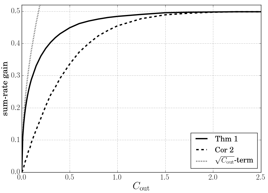
In Figure 2, using [19], we plot the sum-rate of the region 𝒞ach​(Cout)\mathscr{C}_{\mathrm{ach}}(C_{\mathrm{out}}) and the forwarding inner bound (Corollary 2) for γ1=γ2=100\gamma_{1}=\gamma_{2}=100. We also plot the Cout\sqrt{C_{\mathrm{out}}}-term in the lower bound given by Proposition 7. Notice that the forwarding inner bound provides a cooperation gain that is at most linear in CoutC_{\mathrm{out}}.

Refer to caption
Figure 2: Plot of the achievable sum-rate gain given by Theorem 1 and Corollary 2 for Gaussian input distributions, and the Cout\sqrt{C_{\mathrm{out}}}-term given in Proposition 7. Here γ1=γ2=100\gamma_{1}=\gamma_{2}=100.

VI The kk-User MAC with Conferencing Encoders

In this section, we extend Willems’ conferencing encoders model [8] from the 2-user MAC to the kk-user MAC and provide an outer bound on the capacity region.

Consider a kk-user MAC where for every i,j∈[k]i,j\in[k] (in this section, i≠ji\neq j by assumption), there is a noiseless link of capacity Ci​j≥0C_{ij}\geq 0 going from encoder ii to encoder jj and a noiseless link of capacity Cj​i≥0C_{ji}\geq 0 going back (Figure 3).

Refer to caption
Figure 3: In kk-user MAC with conferencing, for every i,j∈[k]i,j\in[k], there are links of capacities Ci​jC_{ij} and Cj​iC_{ji} connecting encoders ii and jj.

As in 2-user conferencing, the “conference” occurs over a finite number of rounds. In the first round, for every i,j∈[k]i,j\in[k] with Ci​j>0C_{ij}>0, encoder ii transmits some information to encoder jj that is a function of its own message wi∈[2n​Ri]w_{i}\in[2^{nR_{i}}]. In each subsequent round, every encoder transmits information that is a function of its message and information it receives before that round. Once the conference is over, each encoder transmits its codeword over the kk-user MAC.

We next define a ((2n​R1,…,2n​Rk),n,L)\big((2^{nR_{1}},\dots,2^{nR_{k}}),n,L\big)-code for the kk-user MAC with an LL-round (Ci​j)i,j=1k(C_{ij})_{i,j=1}^{k}-conference. For every i,j∈[k]i,j\in[k] and ℓ∈[L]\ell\in[L], fix a set 𝒱i​j(ℓ)\mathcal{V}_{ij}^{(\ell)} so that for every i,j∈[k]i,j\in[k], ∑ℓ=1Llog⁡|𝒱i​j(ℓ)|≤n​Ci​j\sum_{\ell=1}^{L}\log|\mathcal{V}_{ij}^{(\ell)}|\leq nC_{ij}. Here 𝒱i​j(ℓ)\mathcal{V}_{ij}^{(\ell)} represents the alphabet of the symbol encoder ii sends to encoder jj in round ℓ\ell of the conference. For every ℓ∈[L]\ell\in[L], define 𝒱i​jℓ=∏ℓ′=1ℓ𝒱i​j(ℓ′)\mathcal{V}_{ij}^{\ell}=\prod_{\ell^{\prime}=1}^{\ell}\mathcal{V}_{ij}^{(\ell^{\prime})}. For j∈[k]j\in[k], encoder jj is represented by the collection of functions (fj,(hj​i(ℓ))i,ℓ)\big(f_{j},(h_{ji}^{(\ell)})_{i,\ell}\big) where

fj\displaystyle f_{j} :[2n​Rj]×∏i:i≠j𝒱i​jL→𝒳jn\displaystyle:[2^{nR_{j}}]\times\prod_{i:i\neq j}\mathcal{V}_{ij}^{L}\rightarrow\mathcal{X}_{j}^{n}
hj​i(ℓ)\displaystyle h_{ji}^{(\ell)} :[2n​Rj]×∏i′:i′≠j𝒱i′​jℓ−1→𝒱j​i(ℓ)\displaystyle:[2^{nR_{j}}]\times\prod_{i^{\prime}:i^{\prime}\neq j}\mathcal{V}_{i^{\prime}j}^{\ell-1}\rightarrow\mathcal{V}_{ji}^{(\ell)}

The decoder is a mapping g:𝒴n→∏j=1k[2n​Rj]g:\mathcal{Y}^{n}\rightarrow\prod_{j=1}^{k}[2^{nR_{j}}]. The definitions of cost constraints, achievable rate vectors, and the capacity region are similar to those given in Section II.

The next result compares the capacity region of a MAC with cooperation under the conferencing and CF models. The proof is given in Subsection VII-F.

Proposition 8.

The capacity region of a MAC with an LL-round (Ci​j)i,j=1k(C_{ij})_{i,j=1}^{k}-conference is a subset of the capacity region of the same MAC with an LL-round (𝐂in,𝐂out)(\mathbf{C}_{\mathrm{in}},\mathbf{C}_{\mathrm{out}})-CF cooperation if for all j∈[k]j\in[k],

Cinj≥∑i:i≠jCj​i\displaystyle C_{\mathrm{in}}^{j}\geq\sum_{i:i\neq j}C_{ji} and Coutj≥∑i:i≠jCi​j.\displaystyle C_{\mathrm{out}}^{j}\geq\sum_{i:i\neq j}C_{ij}.

Similarly, for every LL, the capacity region of a MAC with LL-round (𝐂in,𝐂out)(\mathbf{C}_{\mathrm{in}},\mathbf{C}_{\mathrm{out}})-CF cooperation is a subset of the capacity region of the same MAC with a single-round (Ci​j)i,j=1k(C_{ij})_{i,j=1}^{k}-conference if for all i,j∈[k]i,j\in[k], Ci​j≥CiniC_{ij}\geq C_{\mathrm{in}}^{i}.

Combining the first part of Proposition 8 with the outer bound from Proposition 5 results in the next corollary, which holds regardless of the number of conferencing rounds.

Corollary 9 (Conferencing Outer Bound).

The capacity region of a MAC with a (Ci​j)i,j=1k(C_{ij})_{i,j=1}^{k}-conference is a subset of the set of all rate vectors (R1,…,Rk)(R_{1},\dots,R_{k}) that for some distribution p∈𝒫ind​(𝒰0,𝒳[k])p\in\mathcal{P}_{\mathrm{ind}}(\mathcal{U}_{0},\mathcal{X}_{[k]}), satisfy

∑j∈SRj\displaystyle\sum_{j\in S}R_{j} ≤I(XS;Y|U0,XSc)+∑j∈S∑i≠jCj​i∀∅≠S⊆[k]\displaystyle\leq I\big(X_{S};Y|U_{0},X_{S^{c}}\big)+\sum_{j\in S}\sum_{i\neq j}C_{ji}\qquad\forall\>\emptyset\neq S\subseteq[k]
∑j∈[k]Rj\displaystyle\sum_{j\in[k]}R_{j} ≤I⁡(X[k],Y).\displaystyle\leq I(X_{[k]};Y).

While kk-user conferencing is a direct extension of 2-user conferencing, there is nonetheless an important difference when k≥3k\geq 3. While a single conferencing round suffices to achieve the capacity region in the 2-user case [8], the same is not true when k≥3k\geq 3, as we next see.

A special case of this model for the 3-user Gaussian MAC, depicted in Figure 4(a), is studied in [17]. While the achievability scheme in [17] uses two conferencing rounds, the magnitude of the gain resulting from using an additional conferencing round is not clear. Here, using the idea of a cooperation facilitator, we consider an alternative shown in Figure 4(b), where we show the possibility of a large cooperation gain when conferencing occurs in two rounds rather than one. Consider a 3-user MAC with conferencing. Fix positive constants Cin1C_{\mathrm{in}}^{1} and Cin2C_{\mathrm{in}}^{2}. Let C13=Cin1C_{13}=C^{1}_{\mathrm{in}}, C23=Cin2C_{23}=C^{2}_{\mathrm{in}}, C31=C32=CoutC_{31}=C_{32}=C_{\mathrm{out}} for Cout∈ℝ≥0C_{\mathrm{out}}\in\mathbb{R}_{\geq 0}, and C12=C21=0C_{12}=C_{21}=0.

Refer to caption
Figure 4: (a) The conferencing structure studied in [17]. (b) An example of a structure where allowing two conferencing rounds leads to a substantial gain over a single round.

Let 𝒞1​(Cout)\mathscr{C}_{1}(C_{\mathrm{out}}) and 𝒞2​(Cout)\mathscr{C}_{2}(C_{\mathrm{out}}) denote the capacity region of this network with one and two rounds of conferencing, respectively. For each L∈{1,2}L\in\{1,2\}, define the function gL​(Cout)g_{L}(C_{\mathrm{out}}) as

gL​(Cout)=max(R1,R2,0)∈𝒞L​(Cout)⁡(R1+R2).g_{L}(C_{\mathrm{out}})=\max_{(R_{1},R_{2},0)\in\mathscr{C}_{L}(C_{\mathrm{out}})}(R_{1}+R_{2}).

Note that when L=1L=1, we have g1​(Cout)=g1​(0)g_{1}(C_{\mathrm{out}})=g_{1}(0) for all Cout≥0C_{\mathrm{out}}\geq 0, since no cooperation is possible when encoder 3 is transmitting at rate zero. On the other hand, we next show that at least for some MACs, g2′​(0)=∞g^{\prime}_{2}(0)=\infty; that is, g2g_{2} has an infinite slope at Cout=0C_{\mathrm{out}}=0. Note that

g2​(0)=g1​(0)=maxp⁡(x1)​p​(x2),x3⁡I⁡(X1,X2;Y|X3=x3).g_{2}(0)=g_{1}(0)=\max_{p(x_{1})p(x_{2}),x_{3}}I(X_{1},X_{2};Y|X_{3}=x_{3}).

Suppose x3∗x_{3}^{*} satisfies

maxp⁡(x1)​p​(x2),x3⁡I⁡(X1,X2;Y|X3=x3)=maxp⁡(x1)​p​(x2)⁡I⁡(X1,X2;Y|X3=x3∗).\max_{p(x_{1})p(x_{2}),x_{3}}I(X_{1},X_{2};Y|X_{3}=x_{3})=\max_{p(x_{1})p(x_{2})}I(X_{1},X_{2};Y|X_{3}=x_{3}^{*}).

If the MAC (𝒳1×𝒳2,p⁡(y|x1,x2,x3∗),𝒴)(\mathcal{X}_{1}\times\mathcal{X}_{2},p(y|x_{1},x_{2},x_{3}^{*}),\mathcal{Y}) is in 𝒞∗​(𝒳1×𝒳2,𝒴)\mathcal{C}^{*}(\mathcal{X}_{1}\times\mathcal{X}_{2},\mathcal{Y}), then by Theorem 3, we have g2′​(0)=∞g^{\prime}_{2}(0)=\infty. Since g1g_{1} is constant for all CoutC_{\mathrm{out}}, while g2g_{2} has an infinite slope at Cout=0C_{\mathrm{out}}=0, and g1​(0)=g2​(0)g_{1}(0)=g_{2}(0), the two-round conferencing region is strictly larger than the single-round conferencing region. Using the same technique, we can show a similar result for any k≥3k\geq 3; that is, there exist kk-user MACs where the two-round conferencing region strictly contains the single-round region.

VII Proofs

VII-A Theorem 1 (Inner bound)

Fix η>0\eta>0, and choose a distribution p⁡(u0,u[k],x[k])p(u_{0},u_{[k]},x_{[k]}) on 𝒰0×𝒰[k]×𝒳[k]\mathcal{U}_{0}\times\mathcal{U}_{[k]}\times\mathcal{X}_{[k]} of the form

p⁡(u0)⋅∏i∈Sdcp⁡(ui|u0)⋅p⁡(uSd|u0,uSdc)⋅∏j∈[k]p⁡(xj|u0,uj),p(u_{0})\cdot\prod_{i\in S_{d}^{c}}p(u_{i}|u_{0})\cdot p(u_{S_{d}}|u_{0},u_{S_{d}^{c}})\cdot\prod_{j\in[k]}p(x_{j}|u_{0},u_{j}),

that satisfies the dependence constraints

ζS:=∑j∈SCj​d−∑j∈SH⁡(Uj|U0)+H⁡(US|U0,USdc)>0∀∅⊊S⊆Sd,\zeta_{S}:=\sum_{j\in S}C_{jd}-\sum_{j\in S}H(U_{j}|U_{0})+H(U_{S}|U_{0},U_{S_{d}^{c}})>0\qquad\forall\>\emptyset\subsetneq S\subseteq S_{d},

and cost constraints

𝔼⁡[bj​(Xj)]≤Bj−η∀j∈[k].\mathbb{E}\big[b_{j}(X_{j})\big]\leq B_{j}-\eta\qquad\forall j\in[k]. (16)

Let (w1,…,wk)(w_{1},\dots,w_{k}) denote the transmitted kk-tuple of messages and (W^1,…,W^k)(\hat{W}_{1},\dots,\hat{W}_{k}) denote the output of the decoder. To simplify notation, denote

U0n​(w0),Ujn​(wj​d,Zj|U0n),Xjn​(wj​j|U0n,Ujn)U_{0}^{n}(w_{0}),U_{j}^{n}(w_{jd},Z_{j}|U_{0}^{n}),X_{j}^{n}(w_{jj}|U_{0}^{n},U_{j}^{n})

with U0nU_{0}^{n}, UjnU_{j}^{n}, and XjnX_{j}^{n}, respectively. Similarly, define U^0n\hat{U}_{0}^{n}, U^jn\hat{U}_{j}^{n}, and X^jn\hat{X}_{j}^{n} as

U0n​(W^0),Ujn​(W^j​d,Zj|U0n),Xjn​(W^j​j|U0n,Ujn).U_{0}^{n}(\hat{W}_{0}),U_{j}^{n}(\hat{W}_{jd},Z_{j}|U_{0}^{n}),X_{j}^{n}(\hat{W}_{jj}|U_{0}^{n},U_{j}^{n}).

Here W^0\hat{W}_{0}, W^j​d\hat{W}_{jd}, and W^j​j\hat{W}_{jj} are defined in terms of (W^j)j(\hat{W}_{j})_{j} similar to the definitions of w0w_{0}, wj​dw_{jd}, and wj​jw_{jj} in Section IV. Let YnY^{n} denote the channel output when X[k]nX_{[k]}^{n} is transmitted. Then the joint distribution of (U0n,U[k]n,X[k]n,Yn)(U_{0}^{n},U_{[k]}^{n},X_{[k]}^{n},Y^{n}) is given by

pcode​(u0n,u[k]n,x[k]n,yn)=p⁡(u0n)​pcode​(u[k]n|u0n)​p​(x[k]n|u0n,u[k]n)​p​(yn|x[k]n),p_{\mathrm{code}}(u_{0}^{n},u_{[k]}^{n},x_{[k]}^{n},y^{n})=p(u_{0}^{n})p_{\mathrm{code}}(u_{[k]}^{n}|u_{0}^{n})p(x_{[k]}^{n}|u_{0}^{n},u_{[k]}^{n})p(y^{n}|x_{[k]}^{n}),

where

pcode​(u[k]n|u0n)=∑μ[k]p⁡(μ1|u0n)​…​p​(μk|u0n)​p​(u[k]n|u0n,μ[k])p_{\mathrm{code}}(u_{[k]}^{n}|u_{0}^{n})=\sum_{\mu_{[k]}}p(\mu_{1}|u_{0}^{n})\dots p(\mu_{k}|u_{0}^{n})p(u_{[k]}^{n}|u_{0}^{n},\mu_{[k]})

and p⁡(μj|u0n)p(\mu_{j}|u_{0}^{n}) and p⁡(u[k]n|u0n,μ[k])p(u_{[k]}^{n}|u_{0}^{n},\mu_{[k]}) are calculated according to

p⁡(μj|u0n)=∏zj∈[2n​Cj​d]p⁡(μj​(zj)|u0n),p(\mu_{j}|u_{0}^{n})=\prod_{z_{j}\in[2^{nC_{jd}}]}p(\mu_{j}(z_{j})|u_{0}^{n}),

and

p(u[k]n|u0n,μ[k])=∑z[k]p(z[k]|u0n,μ[k])∏j=1k𝟏{μj(zj)=ujn}.p(u_{[k]}^{n}|u_{0}^{n},\mu_{[k]})=\sum_{z_{[k]}}p(z_{[k]}|u_{0}^{n},\mu_{[k]})\prod_{j=1}^{k}\mathbf{1}\{\mu_{j}(z_{j})=u_{j}^{n}\}.

Define the distribution pind​(u0n,u[k]n,x[k]n,yn)p_{\mathrm{ind}}(u_{0}^{n},u_{[k]}^{n},x_{[k]}^{n},y^{n}) as

pind​(u0n,u[k]n,x[k]n,yn)=p⁡(u0n)​p​(x[k]n|u0n,u[k]n)​p​(yn|x[k]n)​∏j=1kp⁡(ujn|u0n),p_{\mathrm{ind}}(u_{0}^{n},u_{[k]}^{n},x_{[k]}^{n},y^{n})=p(u_{0}^{n})p(x_{[k]}^{n}|u_{0}^{n},u_{[k]}^{n})p(y^{n}|x_{[k]}^{n})\prod_{j=1}^{k}p(u_{j}^{n}|u_{0}^{n}),

which is the joint input-output distribution if independent codewords are transmitted. We next mention some results regarding weakly typical sets that are required for our error analysis.

For any S⊆[k]S\subseteq[k], let Aδ(n)​(U0,US)A_{\delta}^{(n)}(U_{0},U_{S}) denote the weakly typical set with respect to the distribution p⁡(u0,uS)p(u_{0},u_{S}), a marginal of p⁡(u0,u[k])p(u_{0},u_{[k]}). In addition, for every (u0n,uSn)∈Aδ(n)​(U0,US)(u_{0}^{n},u_{S}^{n})\in A_{\delta}^{(n)}(U_{0},U_{S}), let Aδ(n)​(u0n,uSn)A_{\delta}^{(n)}(u_{0}^{n},u_{S}^{n}) be the set of all uScnu_{S^{c}}^{n} such that

(u0n,u[k]n)∈Aδ(n)​(U0,U[k]).(u_{0}^{n},u_{[k]}^{n})\in A_{\delta}^{(n)}(U_{0},U_{[k]}).

Similarly, let Aϵ(n)​(U0,U[k],X[k],Y)A_{\epsilon}^{(n)}(U_{0},U_{[k]},X_{[k]},Y) be the weakly typical set with respect to the distribution p⁡(u0,u[k],x[k])​p​(y|x[k])p(u_{0},u_{[k]},x_{[k]})p(y|x_{[k]}), where p⁡(y|x[k])p(y|x_{[k]}) is given by the channel definition. For subsets S,T⊆[k]S,T\subseteq[k], define Aϵ(n)​(U0,US,XT,Y)A_{\epsilon}^{(n)}(U_{0},U_{S},X_{T},Y) and Aϵ(n)​(u0n,uSn,xTn,yn)A_{\epsilon}^{(n)}(u_{0}^{n},u_{S}^{n},x_{T}^{n},y^{n}) accordingly. If (u0n,uSn,xTn,yn)∈Aϵ(n)​(U0,US,XT,Y)(u_{0}^{n},u_{S}^{n},x_{T}^{n},y^{n})\in A_{\epsilon}^{(n)}(U_{0},U_{S},X_{T},Y), we have [13, p. 523]

log|Aϵ(n)(u0n,uSn,xTn,yn)|≤n(H(USc,XTc|U0,US,XT,Y)+2ϵ).\log|A_{\epsilon}^{(n)}(u_{0}^{n},u_{S}^{n},x_{T}^{n},y^{n})|\leq n\big(H(U_{S^{c}},X_{T^{c}}|U_{0},U_{S},X_{T},Y)+2\epsilon\big). (17)

Finally, under fairly general conditions described in Appendix B,44 4 Distributions that satisfy these conditions include any distribution with finite support and the Gaussian distribution. there exists an increasing function I:ℝ>0→ℝ>0I:\mathbb{R}_{>0}\rightarrow\mathbb{R}_{>0} such that if (U0n,U[k]n,X[k]n,Yn)(U_{0}^{n},U_{[k]}^{n},X_{[k]}^{n},Y^{n}) consists of nn i.i.d. copies of (U0,U[k],X[k],Y)(U_{0},U_{[k]},X_{[k]},Y) distributed according to p⁡(u0,u[k],x[k],y)p(u_{0},u_{[k]},x_{[k]},y), then

Pr{(U0n,U[k]n,X[k]n,Yn)∈Aϵ(n)(U0,U[k],X[k],Y)}≥1−2−nI⁡(ϵ).\pr\Big\{(U_{0}^{n},U_{[k]}^{n},X_{[k]}^{n},Y^{n})\in A_{\epsilon}^{(n)}(U_{0},U_{[k]},X_{[k]},Y)\Big\}\geq 1-2^{-nI(\epsilon)}. (18)

Fix any such function II.

We next study the relationship between pcodep_{\mathrm{code}} and pindp_{\mathrm{ind}}. Our first lemma provides an upper bound for pcodep_{\mathrm{code}} in terms of pindp_{\mathrm{ind}}.

Lemma 10.

For every nonempty S⊆[k]S\subseteq[k] and all (u0n,uSn)(u_{0}^{n},u_{S}^{n}),

1n​log⁡pcode​(uSn|u0n)pind​(uSn|u0n)≤n​CS​d,\frac{1}{n}\log\frac{p_{\mathrm{code}}(u_{S}^{n}|u_{0}^{n})}{p_{\mathrm{ind}}(u_{S}^{n}|u_{0}^{n})}\leq nC_{Sd},

where CS​d=∑j∈SCj​dC_{Sd}=\sum_{j\in S}C_{jd}.

Proof:

Recall

pcode​(uSn|u0n)=∑μ[k]p⁡(uSn|u0n,μ[k])​∏j∈[k]p⁡(μj|u0n).p_{\mathrm{code}}(u_{S}^{n}|u_{0}^{n})=\sum_{\mu_{[k]}}p(u_{S}^{n}|u_{0}^{n},\mu_{[k]})\prod_{j\in[k]}p(\mu_{j}|u_{0}^{n}).

To bound pcode​(uSn|u0n)p_{\mathrm{code}}(u_{S}^{n}|u_{0}^{n}), note that

p(uSn|u0n,μ[k])≤∏j∈S𝟏{μj−1(ujn)≠∅},p(u_{S}^{n}|u_{0}^{n},\mu_{[k]})\leq\prod_{j\in S}\mathbf{1}\big\{\mu_{j}^{-1}(u_{j}^{n})\neq\emptyset\big\},

where

μj−1​(ujn)={zj∈[2n​Cj​d]:μj​(zj)=ujn}.\mu_{j}^{-1}(u_{j}^{n})=\big\{z_{j}\in[2^{nC_{jd}}]:\mu_{j}(z_{j})=u_{j}^{n}\big\}.

Now for every j∈Sj\in S,

∑μjp(μj|u0n)𝟏{μj−1(ujn)≠∅}\displaystyle\sum_{\mu_{j}}p(\mu_{j}|u_{0}^{n})\mathbf{1}\big\{\mu_{j}^{-1}(u_{j}^{n})\neq\emptyset\big\} =Pr{∃zj:Ujn(zj)=ujn|U0n=u0n}\displaystyle=\pr\big\{\exists z_{j}:U_{j}^{n}(z_{j})=u_{j}^{n}|U_{0}^{n}=u_{0}^{n}\big\}
≤2n​Cj​d​p​(ujn|u0n).\displaystyle\leq 2^{nC_{jd}}p(u_{j}^{n}|u_{0}^{n}).

Thus

pcode​(uSn|u0n)\displaystyle p_{\mathrm{code}}(u_{S}^{n}|u_{0}^{n}) ≤∑μS∏j∈Sp(μj|u0n)𝟏{μj−1(ujn)≠∅}\displaystyle\leq\sum_{\mu_{S}}\prod_{j\in S}p(\mu_{j}|u_{0}^{n})\mathbf{1}\big\{\mu_{j}^{-1}(u_{j}^{n})\neq\emptyset\big\}
=∏j∈S(∑μjp(μj|u0n)𝟏{μj−1(ujn)≠∅})\displaystyle=\prod_{j\in S}\Big(\sum_{\mu_{j}}p(\mu_{j}|u_{0}^{n})\mathbf{1}\big\{\mu_{j}^{-1}(u_{j}^{n})\neq\emptyset\big\}\Big)
≤2n​∑j∈SCj​d​pind​(uSn|u0n).\displaystyle\leq 2^{n\sum_{j\in S}C_{jd}}p_{\mathrm{ind}}(u_{S}^{n}|u_{0}^{n}).

∎Our second lemma provides an upper bound for pind​(uSn|u0n)p_{\mathrm{ind}}(u_{S}^{n}|u_{0}^{n}) when (u0n,uSn)(u_{0}^{n},u_{S}^{n}) is typical.

Lemma 11.

For all nonempty Sdc⊆S⊆[k]S_{d}^{c}\subseteq S\subseteq[k] and (u0n,uSn)∈Aδ(n)​(U0,US)(u_{0}^{n},u_{S}^{n})\in A_{\delta}^{(n)}(U_{0},U_{S}),

1nlogpind​(uSn|u0n)p⁡(uSn|u0n)≤−∑j∈S∩SdH(Uj|U0)+H(US∩Sd|U0,USdc)+2(|S∩Sd|+1)δ.\frac{1}{n}\log\frac{p_{\mathrm{ind}}(u_{S}^{n}|u_{0}^{n})}{p(u_{S}^{n}|u_{0}^{n})}\leq-\sum_{j\in S\cap S_{d}}H(U_{j}|U_{0})+H(U_{S\cap S_{d}}|U_{0},U_{S_{d}^{c}})+2(|S\cap S_{d}|+1)\delta.
Proof:

Recall that

p⁡(u[k]n|u0n)=p⁡(uSdn|u0n,uSdcn)​∏j∈Sdcp⁡(ujn|u0n).p(u_{[k]}^{n}|u_{0}^{n})=p(u_{S_{d}}^{n}|u_{0}^{n},u_{S_{d}^{c}}^{n})\prod_{j\in S_{d}^{c}}p(u_{j}^{n}|u_{0}^{n}).

Thus for all S⊇SdcS\supseteq S_{d}^{c}, we have

p⁡(uSn|u0n)=p⁡(uS∩Sdn|u0n,uSdcn)​∏j∈Sdcp⁡(ujn|u0n).p(u_{S}^{n}|u_{0}^{n})=p(u_{S\cap S_{d}}^{n}|u_{0}^{n},u_{S_{d}^{c}}^{n})\prod_{j\in S_{d}^{c}}p(u_{j}^{n}|u_{0}^{n}).

Therefore,

pind​(uSn|u0n)p⁡(uSn|u0n)\displaystyle\frac{p_{\mathrm{ind}}(u_{S}^{n}|u_{0}^{n})}{p(u_{S}^{n}|u_{0}^{n})} =pind​(uS∩Sdn|u0n)p⁡(uS∩Sdn|u0n,uSdcn)\displaystyle=\frac{p_{\mathrm{ind}}(u_{S\cap S_{d}}^{n}|u_{0}^{n})}{p(u_{S\cap S_{d}}^{n}|u_{0}^{n},u_{S_{d}^{c}}^{n})}
=∏j∈S∩Sdp⁡(ujn|u0n)p⁡(uS∩Sdn|u0n,uSdcn).\displaystyle=\frac{\prod_{j\in S\cap S_{d}}p(u_{j}^{n}|u_{0}^{n})}{p(u_{S\cap S_{d}}^{n}|u_{0}^{n},u_{S_{d}^{c}}^{n})}.

The proof now follows from the definition of Aδ(n)​(U0,US)A_{\delta}^{(n)}(U_{0},U_{S}). ∎Combining the previous two lemmas results in the next corollary, which we use in our error analysis.

Corollary 12.

For every nonempty SS satisfying Sdc⊆S⊆[k]S_{d}^{c}\subseteq S\subseteq[k] and all (u0n,uSn)∈Aδ(n)​(U0,US)(u_{0}^{n},u_{S}^{n})\in A_{\delta}^{(n)}(U_{0},U_{S}),

1n​log⁡pcode​(uSn|u0n)p⁡(uSn|u0n)≤ζS∩Sd+2​(|S∩Sd|+1)​δ.\frac{1}{n}\log\frac{p_{\mathrm{code}}(u_{S}^{n}|u_{0}^{n})}{p(u_{S}^{n}|u_{0}^{n})}\leq\zeta_{S\cap S_{d}}+2\big(|S\cap S_{d}|+1\big)\delta.

Let ℰ\mathcal{E} denote the event where either the output of an encoder does not satisfy the corresponding cost constraint, or the output of the decoder differs from the transmitted kk-tuple of messages; that is (W^j)j=1k≠(wj)j=1k(\hat{W}_{j})_{j=1}^{k}\neq(w_{j})_{j=1}^{k}. Denote the former event with ℰcost\mathcal{E}_{\mathrm{cost}} and the latter event with ℰdec\mathcal{E}_{\mathrm{dec}}. When ℰdec\mathcal{E}_{\mathrm{dec}} occurs, it is either the case that (wj)j=1k(w_{j})_{j=1}^{k} does not satisfy (15) (denote this event with ℰtyp\mathcal{E}_{\mathrm{typ}}), or that there is another kk-tuple, (W^j)j=1k≠(wj)j=1k(\hat{W}_{j})_{j=1}^{k}\neq(w_{j})_{j=1}^{k}, that also satisfies (15). If the latter event occurs, we either have W^0≠w0\hat{W}_{0}\neq w_{0} (denote event with ℰ∅,∅\mathcal{E}_{\emptyset,\emptyset}), or W^0=w0\hat{W}_{0}=w_{0}. When W^0=w0\hat{W}_{0}=w_{0}, define the subsets S,T⊆[k]S,T\subseteq[k] as

S\displaystyle S ={j:W^j​d≠wj​d}\displaystyle=\big\{j:\hat{W}_{jd}\neq w_{jd}\big\}
T\displaystyle T ={j:W^j​j≠wj​j}.\displaystyle=\big\{j:\hat{W}_{jj}\neq w_{jj}\big\}.

Now for every pair of subsets S,T⊆[k]S,T\subseteq[k] such that S∪T≠∅S\cup T\neq\emptyset, define ℰS,T\mathcal{E}_{S,T} as the event where there exists a (W^j)j=1k(\hat{W}_{j})_{j=1}^{k} that satisfies (15), W^0=w0\hat{W}_{0}=w_{0}, W^j​d≠wj​d\hat{W}_{jd}\neq w_{jd} if and only if j∈Sj\in S, and W^j​j≠wj​j\hat{W}_{jj}\neq w_{jj} if and only if j∈Tj\in T. Thus we may write

ℰ⊆ℰcost∪ℰtyp∪⋃S,T⊆[k]ℰS,T.\mathcal{E}\subseteq\mathcal{E}_{\mathrm{cost}}\cup\mathcal{E}_{\mathrm{typ}}\cup\bigcup_{S,T\subseteq[k]}\mathcal{E}_{S,T}.

The union over all ℰS,T\mathcal{E}_{S,T} also contains the event ℰ∅,∅\mathcal{E}_{\emptyset,\emptyset}. By the union bound,

Pr⁡(ℰ)≤Pr⁡(ℰcost)+Pr⁡(ℰtyp)+∑S,T⊆[k]Pr⁡(ℰS,T).\pr(\mathcal{E})\leq\pr(\mathcal{E}_{\mathrm{cost}})+\pr(\mathcal{E}_{\mathrm{typ}})+\sum_{S,T\subseteq[k]}\pr(\mathcal{E}_{S,T}).

Thus to find a set of achievable rates for our random code design, it suffices to find conditions under which Pr⁡(ℰcost)\pr(\mathcal{E}_{\mathrm{cost}}), Pr⁡(ℰtyp)\pr(\mathcal{E}_{\mathrm{typ}}), and each Pr⁡(ℰS,T)\pr(\mathcal{E}_{S,T}) go to zero as n→∞n\rightarrow\infty.

We begin our analysis with the event ℰcost\mathcal{E}_{\mathrm{cost}}. For j∈[k]j\in[k], let ℰcostj\mathcal{E}_{\mathrm{cost}}^{j} denote the event where the codeword Xjn​(wj​j|U0n​(w0),Ujn​(wj​d,Zj))X_{j}^{n}(w_{jj}|U_{0}^{n}(w_{0}),U_{j}^{n}(w_{jd},Z_{j})) does not satisfy the cost constraint of encoder jj. We have

Pr⁡(ℰcostj)\displaystyle\pr\big(\mathcal{E}^{j}_{\mathrm{cost}}\big) =Pr{1n∑t=1nbj(Xjt(wjj|U0n(w0),Ujn(wjd,Zj)))>Bj}\displaystyle=\pr\left\{\frac{1}{n}\sum_{t=1}^{n}b_{j}\Big(X_{jt}\big(w_{jj}|U_{0}^{n}(w_{0}),U_{j}^{n}(w_{jd},Z_{j})\big)\Big)>B_{j}\right\}
=∑zjPr{Zj=zj}Pr{1n∑t=1nbj(Xjt(wjj|U0n(w0),Ujn(wjd,zj)))>Bj}.\displaystyle=\sum_{z_{j}}\pr\{Z_{j}=z_{j}\}\pr\left\{\frac{1}{n}\sum_{t=1}^{n}b_{j}\Big(X_{jt}\big(w_{jj}|U_{0}^{n}(w_{0}),U_{j}^{n}(w_{jd},z_{j})\big)\Big)>B_{j}\right\}.

Since for all zjz_{j}, by the AEP,

Pr{1n∑t=1nbj(Xjt(wjj|U0n(w0),Ujn(wjd,zj)))>Bj}→0\pr\left\{\frac{1}{n}\sum_{t=1}^{n}b_{j}\Big(X_{jt}\big(w_{jj}|U_{0}^{n}(w_{0}),U_{j}^{n}(w_{jd},z_{j})\big)\Big)>B_{j}\right\}\rightarrow 0

as n→∞n\rightarrow\infty, it follows that Pr⁡(ℰcostj)→0\pr\big(\mathcal{E}^{j}_{\mathrm{cost}}\big)\rightarrow 0. Applying the union bound now implies

Pr⁡(ℰcost)≤∑j∈[k]Pr⁡(ℰcostj)→0.\pr\big(\mathcal{E}_{\mathrm{cost}}\big)\leq\sum_{j\in[k]}\pr\big(\mathcal{E}^{j}_{\mathrm{cost}}\big)\rightarrow 0.

We next consider the event ℰtyp\mathcal{E}_{\mathrm{typ}}. Define ℰenc\mathcal{E}_{\mathrm{enc}} as the event where

(U0n,U[k]n)∉Aδ(n)​(U0,U[k])\big(U_{0}^{n},U_{[k]}^{n}\big)\notin A_{\delta}^{(n)}(U_{0},U_{[k]})

and note that ℰtyp\mathcal{E}_{\mathrm{typ}} is the event where

(U0n,U[k]n,X[k]n,Yn)∉Aϵ(n)​(U0,U[k],X[k],Y).\big(U_{0}^{n},U_{[k]}^{n},X_{[k]}^{n},Y^{n}\big)\notin A_{\epsilon}^{(n)}(U_{0},U_{[k]},X_{[k]},Y).

The event ℰenc\mathcal{E}_{\mathrm{enc}} occurs if and only if 𝒜(U0n,U[k]n(.))\mathcal{A}(U_{0}^{n},U_{[k]}^{n}(.)) (defined in Section IV) is empty. Thus

Pr(ℰenc)=Pr{𝒜(U0n,U[k]n(.))=∅}.\pr(\mathcal{E}_{\mathrm{enc}})=\pr\big\{\mathcal{A}(U_{0}^{n},U_{[k]}^{n}(.))=\emptyset\big\}.

If Sd=∅S_{d}=\emptyset, Pr⁡(ℰenc)\pr(\mathcal{E}_{\mathrm{enc}}) goes to zero by the AEP since in this case pcode​(u[k]n|u0n)=p⁡(u[k]n|u0n)p_{\mathrm{code}}(u_{[k]}^{n}|u_{0}^{n})=p(u_{[k]}^{n}|u_{0}^{n}). Otherwise, recall that for every nonempty S⊆SdS\subseteq S_{d}, ζS\zeta_{S} is defined as

ζS=∑j∈SCj​d−∑j∈SH⁡(Uj|U0)+H⁡(US|U0,USdc).\zeta_{S}=\sum_{j\in S}C_{jd}-\sum_{j\in S}H(U_{j}|U_{0})+H(U_{S}|U_{0},U_{S_{d}^{c}}).

From the multivariate covering lemma (Appendix A), it follows that Pr⁡(ℰenc)→0\pr(\mathcal{E}_{\mathrm{enc}})\rightarrow 0 if for all nonempty S⊆SdS\subseteq S_{d},

ζS>(8​|Sd|−2​|S|+10)​δ.\zeta_{S}>(8|S_{d}|-2|S|+10)\delta. (19)

Next we find an upper bound for Pr⁡(ℰtyp∖ℰenc)\pr(\mathcal{E}_{\mathrm{typ}}\setminus\mathcal{E}_{\mathrm{enc}}). Let B(n)B^{(n)} be the set of all (u0n,u[k]n,x[k]n,yn)(u_{0}^{n},u_{[k]}^{n},x_{[k]}^{n},y^{n}) such that (u0n,u[k]n)∈Aδ(n)(u_{0}^{n},u_{[k]}^{n})\in A_{\delta}^{(n)} but (u0n,u[k]n,x[k]n,yn)∉Aϵ(n)(u_{0}^{n},u_{[k]}^{n},x_{[k]}^{n},y^{n})\notin A_{\epsilon}^{(n)}. Then

Pr⁡(ℰtyp∖ℰenc)\displaystyle\pr(\mathcal{E}_{\mathrm{typ}}\setminus\mathcal{E}_{\mathrm{enc}}) =∑B(n)p⁡(u0n)​pcode​(u[k]n|u0n)​p​(x[k]n|u0n,u[k]n)​p​(yn|x[k]n)\displaystyle=\sum_{B^{(n)}}p(u_{0}^{n})p_{\mathrm{code}}(u_{[k]}^{n}|u_{0}^{n})p(x_{[k]}^{n}|u_{0}^{n},u_{[k]}^{n})p(y^{n}|x_{[k]}^{n})
≤(a)​2n⁡(ζSd+2​(|Sd|+1)​δ)​∑B(n)p⁡(u0n,u[k]n,x[k]n,yn)\displaystyle\overset{(a)}{\leq}2^{n(\zeta_{S_{d}}+2(|S_{d}|+1)\delta)}\sum_{B^{(n)}}p(u_{0}^{n},u_{[k]}^{n},x_{[k]}^{n},y^{n})
≤(b)​2n⁡(ζSd+2​(|Sd|+1)​δ)​Pr⁡{(Aϵ(n))c}​≤(c)​2n⁡(ζSd+2​(|Sd|+1)​δ−I⁡(ϵ)),\displaystyle\overset{(b)}{\leq}2^{n(\zeta_{S_{d}}+2(|S_{d}|+1)\delta)}\pr\big\{(A_{\epsilon}^{(n)})^{c}\big\}\overset{(c)}{\leq}2^{n(\zeta_{S_{d}}+2(|S_{d}|+1)\delta-I(\epsilon))},

where (a) follows from Corollary 12, (b) holds since B(n)⊆(Aϵ(n))cB^{(n)}\subseteq(A_{\epsilon}^{(n)})^{c}, and (c) follows from the definition of I⁡(ϵ)I(\epsilon) given by (18). Thus Pr⁡(ℰtyp∖ℰenc)→0\pr(\mathcal{E}_{\mathrm{typ}}\setminus\mathcal{E}_{\mathrm{enc}})\rightarrow 0 if

ζSd<I⁡(ϵ)−2​(|Sd|+1)​δ.\zeta_{S_{d}}<I(\epsilon)-2(|S_{d}|+1)\delta. (20)

Therefore, if (19) and (20) both hold, then Pr⁡(ℰtyp)→0\pr(\mathcal{E}_{\mathrm{typ}})\rightarrow 0 since

Pr⁡(ℰtyp)≤Pr⁡(ℰenc∪ℰtyp)=Pr⁡(ℰenc)+Pr⁡(ℰtyp∖ℰenc).\pr(\mathcal{E}_{\mathrm{typ}})\leq\pr(\mathcal{E}_{\mathrm{enc}}\cup\mathcal{E}_{\mathrm{typ}})=\pr(\mathcal{E}_{\mathrm{enc}})+\pr(\mathcal{E}_{\mathrm{typ}}\setminus\mathcal{E}_{\mathrm{enc}}).

We next study ℰ∅,∅\mathcal{E}_{\emptyset,\emptyset}, which is the event where there exists a kk-tuple (W^j)j(\hat{W}_{j})_{j} that satisfies (15) but W^0≠w0\hat{W}_{0}\neq w_{0}. If this event occurs, then (U^0n,U^[k]n,X^[k]n)(\hat{U}_{0}^{n},\hat{U}_{[k]}^{n},\hat{X}_{[k]}^{n}) and YnY^{n} are independent. By the union bound,

Pr⁡(ℰ∅,∅)\displaystyle\pr(\mathcal{E}_{\emptyset,\emptyset}) ≤2n​∑j=1kRj​∑Aϵ(n)pcode​(u0n,u[k]n,x[k]n)​pcode​(yn).\displaystyle\leq 2^{n\sum_{j=1}^{k}R_{j}}\sum_{A_{\epsilon}^{(n)}}p_{\mathrm{code}}(u_{0}^{n},u_{[k]}^{n},x_{[k]}^{n})p_{\mathrm{code}}(y^{n}).

We rewrite the sum in the above inequality as

∑Aϵ(n)​(Y)pcode​(yn)​∑Aϵ(n)​(yn)pcode​(u0n,u[k]n,x[k]n),\sum_{A_{\epsilon}^{(n)}(Y)}p_{\mathrm{code}}(y^{n})\sum_{A_{\epsilon}^{(n)}(y^{n})}p_{\mathrm{code}}(u_{0}^{n},u_{[k]}^{n},x_{[k]}^{n}),

Using Corollary 12, we upper bound the inner sum by

∑Aϵ(n)​(yn)2n⁡(ζSd+2​(|Sd|+1)​δ)​p​(u0n,u[k]n,x[k]n)\displaystyle\sum_{A_{\epsilon}^{(n)}(y^{n})}2^{n(\zeta_{S_{d}}+2(|S_{d}|+1)\delta)}p(u_{0}^{n},u_{[k]}^{n},x_{[k]}^{n})
≤(∗)​2n⁡(H⁡(U0,U[k],X[k]|Y)+2​ϵ)​2n⁡(ζ|Sd|+2​(|Sd|+1)​δ)​2−n⁡(H⁡(U0,U[k],X[k])+ϵ),\displaystyle\overset{(*)}{\leq}2^{n(H(U_{0},U_{[k]},X_{[k]}|Y)+2\epsilon)}2^{n(\zeta_{|S_{d}|}+2(|S_{d}|+1)\delta)}2^{-n(H(U_{0},U_{[k]},X_{[k]})+\epsilon)},

where (∗)(*) follows from (17). This implies Pr⁡(ℰ∅,∅)→0\pr(\mathcal{E}_{\emptyset,\emptyset})\rightarrow 0 if

∑j=1kRj<I⁡(X[k],Y)−ζSd−2​(|Sd|+1)​δ−3​ϵ.\sum_{j=1}^{k}R_{j}<I(X_{[k]};Y)-\zeta_{S_{d}}-2(|S_{d}|+1)\delta-3\epsilon.

Next, let S,T⊆[k]S,T\subseteq[k] be sets such that S∪T≠∅S\cup T\neq\emptyset and consider the event ℰS,T\mathcal{E}_{S,T}. Recall that this is the event where there exists a kk-tuple (W^j)j(\hat{W}_{j})_{j} that satisfies (15) and W^0=w0\hat{W}_{0}=w_{0}, W^j​d≠wj​d\hat{W}_{jd}\neq w_{jd} if and only if j∈Sj\in S, and W^j​j≠wj​j\hat{W}_{jj}\neq w_{jj} if and only if j∈Tj\in T. For every A⊆SA\subseteq S and B⊆ScB\subseteq S^{c}, let ℰS,TA,B⊆ℰS,T\mathcal{E}_{S,T}^{A,B}\subseteq\mathcal{E}_{S,T} be the event where there exists a kk-tuple (W^j)j(\hat{W}_{j})_{j} that satisfies

(U0n​(w0),(Ujn​(W^j​d,Z^j|U0n))j∈A,(Ujn​(wj​d,Z^j|U0n))j∈BCLOSE,\displaystyle\Big(U_{0}^{n}(w_{0}),\big(U_{j}^{n}(\hat{W}_{jd},\hat{Z}_{j}|U_{0}^{n})\big)_{j\in A},\big(U_{j}^{n}(w_{jd},\hat{Z}_{j}|U_{0}^{n})\big)_{j\in B},
OPEN(Xjn​(W^j​j|U0n,U^jn))j∈A∪(B∩T),(Xjn​(wj​j|U0n,U^jn))j∈B∖T,Yn)∈Aϵ(n)\displaystyle\big(X_{j}^{n}(\hat{W}_{jj}|U_{0}^{n},\hat{U}_{j}^{n})\big)_{j\in A\cup(B\cap T)},\big(X_{j}^{n}(w_{jj}|U_{0}^{n},\hat{U}_{j}^{n})\big)_{j\in B\setminus T},Y^{n}\Big)\in A_{\epsilon}^{(n)} (21)

and W^0=w0\hat{W}_{0}=w_{0}, W^j​d≠wj​d\hat{W}_{jd}\neq w_{jd} if and only if j∈Sj\in S, and W^j​j≠wj​j\hat{W}_{jj}\neq w_{jj} if and only if j∈Tj\in T. If ℰS,T\mathcal{E}_{S,T} occurs, then so does ℰS,TA,B\mathcal{E}_{S,T}^{A,B} for every A⊆SA\subseteq S and B⊆ScB\subseteq S^{c}. Thus

ℰS,T⊆⋂A,BℰS,TA,B.\mathcal{E}_{S,T}\subseteq\bigcap_{A,B}\mathcal{E}_{S,T}^{A,B}.

This implies

Pr⁡(ℰS,T)≤minA,B⁡Pr⁡(ℰS,TA,B).\pr(\mathcal{E}_{S,T})\leq\min_{A,B}\pr\big(\mathcal{E}_{S,T}^{A,B}\big). (22)

Therefore, to bound Pr⁡(ℰS,T)\pr(\mathcal{E}_{S,T}), we find an upper bound on Pr⁡(ℰS,TA,B)\pr(\mathcal{E}_{S,T}^{A,B}) for any A⊆SA\subseteq S and B⊆ScB\subseteq S^{c} such that A∪(B∩T)≠∅A\cup(B\cap T)\neq\emptyset. This is the key difference between our error analysis here and the error analysis for the 2-user MAC with transmitter cooperation presented in [1]. For independent distributions, using the constraint that subsets of typical codewords are also typical does not lead to a larger region; the same may not be true when dealing with dependent distributions. That being said, to include all independent random variables in our error analysis, instead of calculating the minimum in (22) over all A⊆SA\subseteq S and B⊆ScB\subseteq S^{c}, we limit ourselves to subsets AA and BB that satisfy

S∩Sdc\displaystyle S\cap S_{d}^{c} ⊆A⊆S\displaystyle\subseteq A\subseteq S
Sc∩Sdc\displaystyle S^{c}\cap S_{d}^{c} ⊆B⊆Sc,\displaystyle\subseteq B\subseteq S^{c},

since all the random vectors (Ujn)j∈Sdc(U_{j}^{n})_{j\in S_{d}^{c}} are independent given U0nU_{0}^{n}. Choose any such AA and BB. Note that for every j∈A∪(B∩T)j\in A\cup(B\cap T), either W^j​d≠wj​d\hat{W}_{jd}\neq w_{jd} or W^j​j≠wj​j\hat{W}_{jj}\neq w_{jj}. In addition, in (21),

((Ujn​(W^j​d,Z^j|U0n))j∈A,(Ujn​(wj​d,Z^j|U0n))j∈BCLOSE,\displaystyle\Big(\big(U_{j}^{n}(\hat{W}_{jd},\hat{Z}_{j}|U_{0}^{n})\big)_{j\in A},\big(U_{j}^{n}(w_{jd},\hat{Z}_{j}|U_{0}^{n})\big)_{j\in B},
OPEN(Xjn​(W^j​j|U0n,Ujn))j∈A∪(B∩T),(Xjn​(wj​j|U0n,Ujn))j∈B∖T)\displaystyle\big(X_{j}^{n}(\hat{W}_{jj}|U_{0}^{n},U_{j}^{n})\big)_{j\in A\cup(B\cap T)},\big(X_{j}^{n}(w_{jj}|U_{0}^{n},U_{j}^{n})\big)_{j\in B\setminus T}\Big)

is independent of YnY^{n} given

(U0n(w0),(Ujn(wj​d,.|U0n))j∈Sc,(Xjn(wj​j|U0n,Ujn(.)))j∈Sc∖T).\Big(U_{0}^{n}(w_{0}),\big(U_{j}^{n}(w_{jd},.|U_{0}^{n})\big)_{j\in S^{c}},\big(X_{j}^{n}(w_{jj}|U_{0}^{n},U_{j}^{n}(.))\big)_{j\in S^{c}\setminus T}\Big).

Therefore, by the union bound, Pr⁡(ℰS,TA,B)\pr(\mathcal{E}_{S,T}^{A,B}) is bounded from above by

2n⁡(∑j∈ARj​d+∑j∈A∪(B∩T)Rj​j)\displaystyle 2^{n\big(\sum_{j\in A}R_{jd}+\sum_{j\in A\cup(B\cap T)}R_{jj}\big)}
×∑Aϵ(n)p⁡(xA∪(B∩T)n|u0n,uA∪(B∩T)n)\displaystyle\times\sum_{A_{\epsilon}^{(n)}}p(x_{A\cup(B\cap T)}^{n}|u_{0}^{n},u_{A\cup(B\cap T)}^{n})
×∑μA∪Sc,χSc∖Tp(u0n,μSc,χSc∖T,yn)p(μA|u0n)p(uA∪Bn,xB∖Tn|u0n,μA∪Sc,χSc∖T),\displaystyle\phantom{\times\sum_{A_{\epsilon}^{(n)}}}\times\sum_{\mu_{A\cup S^{c}},\chi_{S^{c}\setminus T}}p(u_{0}^{n},\mu_{S^{c}},\chi_{S^{c}\setminus T},y^{n})p(\mu_{A}|u_{0}^{n})p(u_{A\cup B}^{n},x_{B\setminus T}^{n}|u_{0}^{n},\mu_{A\cup S^{c}},\chi_{S^{c}\setminus T}), (23)

where the inner sum is over all mappings μj:[2n​Cj​d]→𝒰jn\mu_{j}:[2^{nC_{jd}}]\rightarrow\mathcal{U}_{j}^{n} for j∈A∪Scj\in A\cup S^{c} and χj:[2n​Cj​d]→𝒳jn\chi_{j}:[2^{nC_{jd}}]\rightarrow\mathcal{X}_{j}^{n} for j∈Sc∖Tj\in S^{c}\setminus T. The distribution p⁡(u0n,μSc,χSc∖T,yn)p(u_{0}^{n},\mu_{S^{c}},\chi_{S^{c}\setminus T},y^{n}) is a marginal of p⁡(u0n,μ[k],χ[k],yn)p(u_{0}^{n},\mu_{[k]},\chi_{[k]},y^{n}), which is defined as

p⁡(u0n,μ[k],χ[k],yn)=p⁡(u0n,μ[k])​p​(χ[k]|u0n,μ[k])​p​(yn|u0n,μ[k],χ[k]),p(u_{0}^{n},\mu_{[k]},\chi_{[k]},y^{n})=p(u_{0}^{n},\mu_{[k]})p(\chi_{[k]}|u_{0}^{n},\mu_{[k]})p(y^{n}|u_{0}^{n},\mu_{[k]},\chi_{[k]}),

where

p⁡(χ[k]|u0n,μ[k])\displaystyle p(\chi_{[k]}|u_{0}^{n},\mu_{[k]}) =∏j∈[k]p⁡(χj|u0n,μj)\displaystyle=\prod_{j\in[k]}p(\chi_{j}|u_{0}^{n},\mu_{j})
=∏j∈[k]∏zj∈[2n​Cj​d]p⁡(χj​(zj)|u0n,μj​(zj)),\displaystyle=\prod_{j\in[k]}\prod_{z_{j}\in[2^{nC_{jd}}]}p(\chi_{j}(z_{j})|u_{0}^{n},\mu_{j}(z_{j})),

and

p⁡(yn|u0n,μ[k],χ[k])=∑z[k]p⁡(z[k]|u0n,μ[k])​p​(yn|χ[k]​(z[k])).p(y^{n}|u_{0}^{n},\mu_{[k]},\chi_{[k]})=\sum_{z_{[k]}}p(z_{[k]}|u_{0}^{n},\mu_{[k]})p(y^{n}|\chi_{[k]}(z_{[k]})).

We have

p(uA∪Bn,xB∖Tn|u0n,μA∪Sc,χSc∖T)\displaystyle p(u_{A\cup B}^{n},x_{B\setminus T}^{n}|u_{0}^{n},\mu_{A\cup S^{c}},\chi_{S^{c}\setminus T})
≤𝟏{∃(zj)j∈B∈∏j∈B[2n​Cj​d]:(∀j∈B:μj(zj)=ujn)∧(∀j∈B∖T:χj(zj)=xjn)}\displaystyle\leq\mathbf{1}\Big\{\exists(z_{j})_{j\in B}\in\prod_{j\in B}[2^{nC_{jd}}]:(\forall j\in B:\mu_{j}(z_{j})=u_{j}^{n})\wedge(\forall j\in B\setminus T:\chi_{j}(z_{j})=x_{j}^{n})\Big\}
×𝟏{∃(zj)j∈A∈∏j∈A[2n​Cj​d]:(∀j∈A:μj(zj)=ujn)}.\displaystyle\phantom{\leq}\times\mathbf{1}\Big\{\exists(z_{j})_{j\in A}\in\prod_{j\in A}[2^{nC_{jd}}]:(\forall j\in A:\mu_{j}(z_{j})=u_{j}^{n})\Big\}. (24)

We can thus upper bound the inner sum in (23) as a product of the sums

∑μSc,χSc∖Tp⁡(u0n,μSc,χSc∖T,yn)\displaystyle\sum_{\mu_{S^{c}},\chi_{S^{c}\setminus T}}p(u_{0}^{n},\mu_{S^{c}},\chi_{S^{c}\setminus T},y^{n})
×𝟏{∃(zj)j∈B∈∏j∈B[2n​Cj​d]:(∀j∈B:μj(zj)=ujn)∧(∀j∈B∖T:χj(zj)=xjn)}\displaystyle\times\mathbf{1}\Big\{\exists(z_{j})_{j\in B}\in\prod_{j\in B}[2^{nC_{jd}}]:(\forall j\in B:\mu_{j}(z_{j})=u_{j}^{n})\wedge(\forall j\in B\setminus T:\chi_{j}(z_{j})=x_{j}^{n})\Big\}

and

∑μAp(μA|u0n)𝟏{∃(zj)j∈A∈∏j∈A[2n​Cj​d]:∀j∈A,μj(zj)=ujn}.\sum_{\mu_{A}}p(\mu_{A}|u_{0}^{n})\mathbf{1}\Big\{\exists(z_{j})_{j\in A}\in\prod_{j\in A}[2^{nC_{jd}}]:\forall j\in A,\mu_{j}(z_{j})=u_{j}^{n}\Big\}.

We first find an upper bound for the first sum. Define the distribution p~​(u0n,u[k]n,x[k]n,yn)\tilde{p}(u_{0}^{n},u_{[k]}^{n},x_{[k]}^{n},y^{n}) as

p~​(u0n,u[k]n,x[k]n,yn)=∑μ[k],χ[k]p⁡(u0n,μ[k],χ[k],yn)​∏j=1k𝟏​{μj​(1)=ujn,χj​(1)=xjn}.\tilde{p}(u_{0}^{n},u_{[k]}^{n},x_{[k]}^{n},y^{n})=\sum_{\mu_{[k]},\chi_{[k]}}p(u_{0}^{n},\mu_{[k]},\chi_{[k]},y^{n})\prod_{j=1}^{k}\mathbf{1}\big\{\mu_{j}(1)=u_{j}^{n},\chi_{j}(1)=x_{j}^{n}\big\}.

The following argument demonstrates that p~​(u0n,u[k]n,x[k]n)=pind​(u0n,u[k]n,x[k]n)\tilde{p}(u_{0}^{n},u_{[k]}^{n},x_{[k]}^{n})=p_{\mathrm{ind}}(u_{0}^{n},u_{[k]}^{n},x_{[k]}^{n}),

p~​(u0n,u[k]n,x[k]n)\displaystyle\tilde{p}(u_{0}^{n},u_{[k]}^{n},x_{[k]}^{n}) =∑ynp~​(u0n,u[k]n,x[k]n,yn)\displaystyle=\sum_{y^{n}}\tilde{p}(u_{0}^{n},u_{[k]}^{n},x_{[k]}^{n},y^{n})
=∑μ[k],χ[k]p⁡(u0n,μ[k],χ[k])​∏j=1k𝟏​{μj​(1)=ujn,χj​(1)=xjn}\displaystyle=\sum_{\mu_{[k]},\chi_{[k]}}p(u_{0}^{n},\mu_{[k]},\chi_{[k]})\prod_{j=1}^{k}\mathbf{1}\big\{\mu_{j}(1)=u_{j}^{n},\chi_{j}(1)=x_{j}^{n}\big\}
=p⁡(u0n)​∏j=1k∑μj,χjp⁡(μj,χj|u0n)​𝟏​{μj​(1)=ujn,χj​(1)=xjn}\displaystyle=p(u_{0}^{n})\prod_{j=1}^{k}\sum_{\mu_{j},\chi_{j}}p(\mu_{j},\chi_{j}|u_{0}^{n})\mathbf{1}\big\{\mu_{j}(1)=u_{j}^{n},\chi_{j}(1)=x_{j}^{n}\big\}
=pind​(u0n,u[k]n,x[k]n).\displaystyle=p_{\mathrm{ind}}(u_{0}^{n},u_{[k]}^{n},x_{[k]}^{n}). (25)

For every 𝐳=(zj)j∈B\mathbf{z}=(z_{j})_{j\in B}, where zj∈[2n​Cj​d]z_{j}\in[2^{nC_{jd}}] for all j∈Bj\in B, let E𝐳E_{\mathbf{z}} denote the event where for all j∈Bj\in B, Ujn​(wj​d,zj|U0n)=ujnU_{j}^{n}(w_{jd},z_{j}|U_{0}^{n})=u_{j}^{n}, and for all j∈B∖Tj\in B\setminus T, Xjn​(wj​j|U0n,Ujn)=xjnX_{j}^{n}(w_{jj}|U_{0}^{n},U_{j}^{n})=x_{j}^{n}. Then

∑μSc,χSc∖Tp⁡(u0n,μSc,χSc∖T,yn)\displaystyle\sum_{\mu_{S^{c}},\chi_{S^{c}\setminus T}}p(u_{0}^{n},\mu_{S^{c}},\chi_{S^{c}\setminus T},y^{n})
×𝟏{∃𝐳∈∏j∈B[2n​Cj​d]:(∀j∈B:μj(zj)=ujn)∧(∀j∈B∖T:χj(zj)=xjn)}\displaystyle\times\mathbf{1}\Big\{\exists\mathbf{z}\in\prod_{j\in B}[2^{nC_{jd}}]:(\forall j\in B:\mu_{j}(z_{j})=u_{j}^{n})\wedge(\forall j\in B\setminus T:\chi_{j}(z_{j})=x_{j}^{n})\Big\}
=Pr⁡({U0n=u0n,Yn=yn}∩⋃𝐳E𝐳)\displaystyle=\pr\Big(\{U_{0}^{n}=u_{0}^{n},Y^{n}=y^{n}\}\cap\bigcup_{\mathbf{z}}E_{\mathbf{z}}\Big)
=Pr⁡(⋃𝐳({U0n=u0n,Yn=yn}∩E𝐳))\displaystyle=\pr\Big(\bigcup_{\mathbf{z}}\big(\{U_{0}^{n}=u_{0}^{n},Y^{n}=y^{n}\}\cap E_{\mathbf{z}}\big)\Big)
≤(a)​2n​CB​d​Pr⁡({U0n=u0n,Yn=yn}∩E𝐳=𝟏)\displaystyle\overset{(a)}{\leq}2^{nC_{Bd}}\pr\big(\{U_{0}^{n}=u_{0}^{n},Y^{n}=y^{n}\}\cap E_{\mathbf{z}=\mathbf{1}}\big)
=2n​CB​d​p~​(u0n,uBn,xB∖Tn,yn)\displaystyle=2^{nC_{Bd}}\tilde{p}(u_{0}^{n},u_{B}^{n},x_{B\setminus T}^{n},y^{n})
=(b)​2n​CB​d​p​(u0n)​pind​(uBn,xB∖Tn|u0n)​p~​(yn|u0n,uBn,xB∖Tn),\displaystyle\overset{(b)}{=}2^{nC_{Bd}}p(u_{0}^{n})p_{\mathrm{ind}}(u_{B}^{n},x_{B\setminus T}^{n}|u_{0}^{n})\tilde{p}(y^{n}|u_{0}^{n},u_{B}^{n},x_{B\setminus T}^{n}), (26)

where (a)(a) follows by the union bound and (b)(b) follows by (25). Using a similar argument we can show

∑μAp(μA|u0n)𝟏{∃𝐳∈∏j∈A[2n​Cj​d]:∀j∈A,μj(zj)=ujn}≤2n​CA​dpind(uAn|u0n).\sum_{\mu_{A}}p(\mu_{A}|u_{0}^{n})\mathbf{1}\Big\{\exists\mathbf{z}\in\prod_{j\in A}[2^{nC_{jd}}]:\forall j\in A,\mu_{j}(z_{j})=u_{j}^{n}\Big\}\leq 2^{nC_{Ad}}p_{\mathrm{ind}}(u_{A}^{n}|u_{0}^{n}). (27)

Thus by (24), (26), and (27), the expression

2n⁡(∑j∈ARj​d+∑j∈A∪(B∩T)Rj​j+CA​d+CB​d)\displaystyle 2^{n\big(\sum_{j\in A}R_{jd}+\sum_{j\in A\cup(B\cap T)}R_{jj}+C_{Ad}+C_{Bd}\big)}
×∑Aϵ(n)p⁡(u0n)​pind​(uA∪Bn|u0n)​p​(xA∪Bn|u0n,uA∪Bn)​p~​(yn|u0n,uBn,xB∖Tn)\displaystyle\times\sum_{A_{\epsilon}^{(n)}}p(u_{0}^{n})p_{\mathrm{ind}}(u_{A\cup B}^{n}|u_{0}^{n})p(x_{A\cup B}^{n}|u_{0}^{n},u_{A\cup B}^{n})\tilde{p}(y^{n}|u_{0}^{n},u_{B}^{n},x_{B\setminus T}^{n})

is an upper bound for (23). Applying Lemma 11 to pind​(uA∪Bn|u0n)p_{\mathrm{ind}}(u_{A\cup B}^{n}|u_{0}^{n}) and dropping the epsilon term, this expression can be further bounded from above by

2n⁡(∑j∈ARj​d+∑j∈A∪(B∩T)Rj​j+ζ(A∪B)∩Sd)\displaystyle 2^{n\big(\sum_{j\in A}R_{jd}+\sum_{j\in A\cup(B\cap T)}R_{jj}+\zeta_{(A\cup B)\cap S_{d}}\big)}
×∑Aϵ(n)​(U0,UB,XB∖T,Y)p⁡(u0n,uBn,xB∖Tn)​p~​(yn|u0n,uBn,xB∖Tn)\displaystyle\phantom{=}\times\sum_{A_{\epsilon}^{(n)}(U_{0},U_{B},X_{B\setminus T},Y)}p(u_{0}^{n},u_{B}^{n},x_{B\setminus T}^{n})\tilde{p}(y^{n}|u_{0}^{n},u_{B}^{n},x_{B\setminus T}^{n})
×∑Aϵ(n)​(u0n,uBn,xB∖Tn,yn)p⁡(uAn|u0n,uBn)​p​(xA∪(B∩T)n|u0n,uA∪(B∩T)n)\displaystyle\phantom{=}\times\sum_{A_{\epsilon}^{(n)}(u_{0}^{n},u_{B}^{n},x_{B\setminus T}^{n},y^{n})}p(u_{A}^{n}|u_{0}^{n},u_{B}^{n})p(x_{A\cup(B\cap T)}^{n}|u_{0}^{n},u_{A\cup(B\cap T)}^{n})

Using (17), we can further upper bound the logarithm of this expression by

n⁡[∑j∈ARj​d+∑j∈A∪(B∩T)Rj​j+ζ(A∪B)∩Sd]\displaystyle n\bigg[\sum_{j\in A}R_{jd}+\sum_{j\in A\cup(B\cap T)}R_{jj}+\zeta_{(A\cup B)\cap S_{d}}\bigg]
+log∑Aϵ(n)​(U0,UB,XB∖T,Y)p(u0n,uBn,xB∖Tn)p~(yn|u0n,uBn,xB∖Tn)\displaystyle+\log\sum_{A_{\epsilon}^{(n)}(U_{0},U_{B},X_{B\setminus T},Y)}p(u_{0}^{n},u_{B}^{n},x_{B\setminus T}^{n})\tilde{p}(y^{n}|u_{0}^{n},u_{B}^{n},x_{B\setminus T}^{n})
−n​H​(UA|U0,UB)−n​H​(XA∪(B∩T)|U0,UA∪(B∩T))\displaystyle-nH(U_{A}|U_{0},U_{B})-nH(X_{A\cup(B\cap T)}|U_{0},U_{A\cup(B\cap T)})
+nH(UA,XA∪(B∩T)|U0,UB,XB∖T,Y)\displaystyle+nH(U_{A},X_{A\cup(B\cap T)}|U_{0},U_{B},X_{B\setminus T},Y)

Hence Pr⁡(ℰS,TA,B)→0\pr(\mathcal{E}_{S,T}^{A,B})\rightarrow 0 if

∑j∈ARj​d+∑j∈A∪(B∩T)Rj​j\displaystyle\sum_{j\in A}R_{jd}+\sum_{j\in A\cup(B\cap T)}R_{jj}
<−ζ(A∪B)∩Sd+H⁡(UA|U0,UB)+H⁡(XA∪(B∩T)|U0,UA∪(B∩T))\displaystyle<-\zeta_{(A\cup B)\cap S_{d}}+H(U_{A}|U_{0},U_{B})+H(X_{A\cup(B\cap T)}|U_{0},U_{A\cup(B\cap T)})
−H(UA,XA∪(B∩T)|U0,UB,XB∖T,Y)\displaystyle\phantom{<}-H(U_{A},X_{A\cup(B\cap T)}|U_{0},U_{B},X_{B\setminus T},Y)
=I(UA,XA∪(B∩T);Y|U0,UB,XB∖T)−ζ(A∪B)∩Sd,\displaystyle=I(U_{A},X_{A\cup(B\cap T)};Y|U_{0},U_{B},X_{B\setminus T})-\zeta_{(A\cup B)\cap S_{d}},

where the last equality follows from the fact that

H⁡(UA|U0,UB)\displaystyle H(U_{A}|U_{0},U_{B}) =H(UA|U0,UB,XB∖T)+I(UA;XB∖T|U0,UB)\displaystyle=H(U_{A}|U_{0},U_{B},X_{B\setminus T})+I(U_{A};X_{B\setminus T}|U_{0},U_{B})
=H⁡(UA|U0,UB,XB∖T)\displaystyle=H(U_{A}|U_{0},U_{B},X_{B\setminus T})

and

H⁡(XA∪(B∩T)|U0,UA∪B)\displaystyle H(X_{A\cup(B\cap T)}|U_{0},U_{A\cup B}) =H(XA∪(B∩T)|U0,UA∪B,XB∖T)+I(XA∪(B∩T);XB∖T|U0,UA∪B)\displaystyle=H(X_{A\cup(B\cap T)}|U_{0},U_{A\cup B},X_{B\setminus T})+I(X_{A\cup(B\cap T)};X_{B\setminus T}|U_{0},U_{A\cup B})
=H⁡(XA∪(B∩T)|U0,UA∪B,XB∖T).\displaystyle=H(X_{A\cup(B\cap T)}|U_{0},U_{A\cup B},X_{B\setminus T}).

Thus Pr⁡(ℰS,T)→0\pr(\mathcal{E}_{S,T})\rightarrow 0 if for some S∩Sdc⊆A⊆SS\cap S_{d}^{c}\subseteq A\subseteq S and Sc∩Sdc⊆B⊆ScS^{c}\cap S_{d}^{c}\subseteq B\subseteq S^{c} such that A∪(B∩T)≠∅A\cup(B\cap T)\neq\emptyset,

∑j∈ARj​d+∑j∈A∪(B∩T)Rj​j\displaystyle\sum_{j\in A}R_{jd}+\sum_{j\in A\cup(B\cap T)}R_{jj}
<I(UA,XA∪(B∩T);Y|U0,UB,XB∖T)−ζ(A∪B)∩Sd\displaystyle<I(U_{A},X_{A\cup(B\cap T)};Y|U_{0},U_{B},X_{B\setminus T})-\zeta_{(A\cup B)\cap S_{d}} (28)

The bounds we obtain above are in terms of (Rj​d)j=1k(R_{jd})_{j=1}^{k} and (Rj​j)j=1k(R_{jj})_{j=1}^{k}. To convert these to bounds in terms of (Rj)j=1k(R_{j})_{j=1}^{k}, recall that Rj​0=min⁡{Cj​0,Rj}R_{j0}=\min\{C_{j0},R_{j}\}, Rj​j=(Rj−Cinj)+R_{jj}=(R_{j}-C_{\mathrm{in}}^{j})^{+}, and

Rj​d\displaystyle R_{jd} =Rj−Rj​0−Rj​j\displaystyle=R_{j}-R_{j0}-R_{jj}
=Rj−min⁡{Cj​0,Rj}−Rj​j=max⁡{Rj−Cj​0,0}−(Rj−Cinj)+\displaystyle=R_{j}-\min\{C_{j0},R_{j}\}-R_{jj}=\max\{R_{j}-C_{j0},0\}-(R_{j}-C_{\mathrm{in}}^{j})^{+}
=(Rj−Cj​0)+−(Rj−Cinj)+.\displaystyle=(R_{j}-C_{j0})^{+}-(R_{j}-C_{\mathrm{in}}^{j})^{+}.

Thus (28) can be written as

∑j∈A(Rj−Cj​0)++∑j∈B∩T(Rj−Cinj)+\displaystyle\sum_{j\in A}(R_{j}-C_{j0})^{+}+\sum_{j\in B\cap T}(R_{j}-C_{\mathrm{in}}^{j})^{+}
<I(UA,XA∪(B∩T);Y|U0,UB,XB∖T)−ζ(A∪B)∩Sd\displaystyle<I(U_{A},X_{A\cup(B\cap T)};Y|U_{0},U_{B},X_{B\setminus T})-\zeta_{(A\cup B)\cap S_{d}}

VII-B Theorem 3 (Sum-capacity gain)

Fix any unit vector 𝐯∈ℝ>0k\mathbf{v}\in\mathbb{R}^{k}_{>0}, rate vector 𝐂in∈ℝ>0k\mathbf{C}_{\mathrm{in}}\in\mathbb{R}^{k}_{>0}, and 𝐁∈ℝ≥0k\mathbf{B}\in\mathbb{R}^{k}_{\geq 0}. For every h≥0h\geq 0, define 𝐂out​(h)=h​𝐯\mathbf{C}_{\mathrm{out}}(h)=h\mathbf{v}. In the achievable region defined in Section II, let 𝒰0={0,1}\mathcal{U}_{0}=\{0,1\}, and for every j∈[k]j\in[k], let 𝒰j=𝒳j\mathcal{U}_{j}=\mathcal{X}_{j}. Set Cj​0=0C_{j0}=0 and Cj​d=Coutj​(h)C_{jd}=C_{\mathrm{out}}^{j}(h) for every j∈[k]j\in[k]. For h>0h>0, let 𝒫⁡(h)\mathcal{P}(h) be the set of all distributions of the form

p⁡(u0,u[k])⋅∏j∈[k]p⁡(xj|u0,uj)p(u_{0},u_{[k]})\cdot\prod_{j\in[k]}p(x_{j}|u_{0},u_{j})

that satisfy dependence constraints

∑j∈SCoutj​(h)−∑j∈SH⁡(Uj|U0)+H⁡(US|U0)>0∀∅⊊S⊆[k],\sum_{j\in S}C_{\mathrm{out}}^{j}(h)-\sum_{j\in S}H(U_{j}|U_{0})+H(U_{S}|U_{0})>0\qquad\forall\>\emptyset\subsetneq S\subseteq[k],

and cost constraints

𝔼⁡[bj​(Xj)]≤Bj∀j∈[k].\mathbb{E}\big[b_{j}(X_{j})\big]\leq B_{j}\qquad\forall j\in[k].

Using Lemma 13 (see end of this section), we see that every rate vector (Rj)j∈[k](R_{j})_{j\in[k]} that for some distribution p∈𝒫⁡(h)p\in\mathcal{P}(h) and every pair of subsets S,T⊆[k]S,T\subseteq[k] satisfies

∑j∈S∪TRj<I(XS∪T;Y|U0,USc,XSc∩Tc)+∑j∈T∖SCinj−ζ[k]\sum_{j\in S\cup T}R_{j}<I(X_{S\cup T};Y|U_{0},U_{S^{c}},X_{S^{c}\cap T^{c}})+\sum_{j\in T\setminus S}C_{\mathrm{in}}^{j}-\zeta_{[k]} (29)

and

∑j∈[k]Rj<I⁡(X[k],Y)−ζ[k],\sum_{j\in[k]}R_{j}<I(X_{[k]};Y)-\zeta_{[k]},

is achievable. This follows from setting A=SA=S and B=ScB=S^{c} for every S,T⊆[k]S,T\subseteq[k] in (8). To obtain a lower bound on sum-capacity, we evaluate this region for a specific distribution in 𝒫⁡(h)\mathcal{P}(h).

Since our MAC is in 𝒞∗​(𝒳[k],𝒴)\mathcal{C}^{*}(\mathcal{X}_{[k]},\mathcal{Y}), there exists a distribution pa∈𝒫ind​(𝒳[k])p_{a}\in\mathcal{P}_{\mathrm{ind}}(\mathcal{X}_{[k]}) that satisfies

Ia​(X[k],Y)=maxp∈𝒫ind​(𝒳[k])⁡I⁡(X[k],Y),I_{a}(X_{[k]};Y)=\max_{p\in\mathcal{P}_{\mathrm{ind}}(\mathcal{X}_{[k]})}I(X_{[k]};Y),

and a distribution pb∈𝒫⁡(𝒳[k])p_{b}\in\mathcal{P}(\mathcal{X}_{[k]}) that satisfies

𝔼b[D(p(y|X[k])∥pa(y))]>𝔼a[D(p(y|X[k])∥pa(y))],\mathbb{E}_{b}\Big[D\big(p(y|X_{[k]})\|p_{a}(y)\big)\Big]>\mathbb{E}_{a}\Big[D\big(p(y|X_{[k]})\|p_{a}(y)\big)\Big],

and whose support is contained in the support of pap_{a}. Here we also assume that for all j∈[k]j\in[k],

Ia​(Xj;Y|X[k]∖{j})>0.I_{a}(X_{j};Y|X_{[k]\setminus\{j\}})>0.

At the end of the proof, we show that in the case where this property does not hold, the same result follows by considering a MAC with a smaller number of users.

Choose μ∈(0,1)\mu\in(0,1) such that for every nonempty S⊆[k]S\subseteq[k],

μ​Ia​(XS;Y|XSc)<∑j∈SCinj.\mu I_{a}(X_{S};Y|X_{S^{c}})<\sum_{j\in S}C_{\mathrm{in}}^{j}. (30)

For every λ∈[0,1]\lambda\in[0,1], define the distribution pλ​(u0,u[k],x[k])p_{\lambda}(u_{0},u_{[k]},x_{[k]}) as

pλ​(u0,u[k],x[k])=pλ​(u0)​pλ​(u[k])​pλ​(x[k]|u0,u[k]),p_{\lambda}(u_{0},u_{[k]},x_{[k]})=p_{\lambda}(u_{0})p_{\lambda}(u_{[k]})p_{\lambda}(x_{[k]}|u_{0},u_{[k]}),

where

pλ​(u0)={μif ​u0=11−μif ​u0=0,p_{\lambda}(u_{0})=\begin{cases}\mu&\text{if }u_{0}=1\\ 1-\mu&\text{if }u_{0}=0,\end{cases}

and for every u[k]∈𝒰[k]u_{[k]}\in\mathcal{U}_{[k]} (recall 𝒰[k]=𝒳[k]\mathcal{U}_{[k]}=\mathcal{X}_{[k]}),

pλ​(u[k])=(1−λ)​pa​(u[k])+λ​pb​(u[k]).p_{\lambda}(u_{[k]})=(1-\lambda)p_{a}(u_{[k]})+\lambda p_{b}(u_{[k]}).

Finally, for every (u0,u[k],x[k])(u_{0},u_{[k]},x_{[k]}),

pλ​(x[k]|u0,u[k])=∏j=1kpλ​(xj|u0,uj),p_{\lambda}(x_{[k]}|u_{0},u_{[k]})=\prod_{j=1}^{k}p_{\lambda}(x_{j}|u_{0},u_{j}),

where for all j∈[k]j\in[k],

pλ​(xj|u0,uj)={𝟏{xj=uj}if ​u0=1pa​(xj)if ​u0=0.p_{\lambda}(x_{j}|u_{0},u_{j})=\begin{cases}\mathbf{1}\{x_{j}=u_{j}\}&\text{if }u_{0}=1\\ p_{a}(x_{j})&\text{if }u_{0}=0.\end{cases}

Note that pλ​(u0)p_{\lambda}(u_{0}) and pλ​(x[k]|u0,u[k])p_{\lambda}(x_{[k]}|u_{0},u_{[k]}) do not depend on λ\lambda. In addition, since pap_{a} and pbp_{b} satisfy the cost constraints and

pλ​(x[k])=(1−λ)​pa​(x[k])+λ​pb​(x[k]),p_{\lambda}(x_{[k]})=(1-\lambda)p_{a}(x_{[k]})+\lambda p_{b}(x_{[k]}),

for all λ∈(0,1)\lambda\in(0,1), pλp_{\lambda} satisfies the cost constraints as well.

We next find a function λ∗​(h)\lambda^{*}(h) so that

pλ∗​(h)​(u0,u[k],x[k])∈𝒫⁡(h)p_{\lambda^{*}(h)}(u_{0},u_{[k]},x_{[k]})\in\mathcal{P}(h)

for sufficiently small hh. Fix ϵ>0\epsilon>0, and consider the equation

h​∑j∈[k]vj=∑j∈[k]Hλ​(Uj)−Hλ​(U[k])+ϵ​λ​∑j∈[k]vj.h\sum_{j\in[k]}v_{j}=\sum_{j\in[k]}H_{\lambda}(U_{j})-H_{\lambda}(U_{[k]})+\epsilon\lambda\sum_{j\in[k]}v_{j}. (31)

By Lemma 14 (see end of this section),

d​hd​λ|λ=0+=ϵ>0.\frac{dh}{d\lambda}\Big|_{\lambda=0^{+}}=\epsilon>0.

Thus the inverse function theorem implies that there exists a function λ=λ∗​(h)\lambda=\lambda^{*}(h) defined on [0,h0)[0,h_{0}) for some h0>0h_{0}>0 that satisfies (31), and

d​λ∗d​h|h=0+=1ϵ.\frac{d\lambda^{*}}{dh}\Big|_{h=0^{+}}=\frac{1}{\epsilon}. (32)

For every nonempty S⊆[k]S\subseteq[k], define the function ζS:[0,h0)→ℝ\zeta_{S}:[0,h_{0})\rightarrow\mathbb{R} as

ζS​(h)=∑j∈SCoutj​(h)−∑j∈SHλ∗​(Uj)+Hλ∗​(US),\zeta_{S}(h)=\sum_{j\in S}C^{j}_{\mathrm{out}}(h)-\sum_{j\in S}H_{\lambda^{*}}(U_{j})+H_{\lambda^{*}}(U_{S}), (33)

If we calculate the derivative of ζS\zeta_{S} at h=0h=0, by Lemma 14, we get

d​ζSd​h|h=0+=∑j∈Svj>0.\frac{d\zeta_{S}}{dh}\Big|_{h=0^{+}}=\sum_{j\in S}v_{j}>0.

This implies that there exists 0<h1≤h00<h_{1}\leq h_{0} such that for every 0<h<h10<h<h_{1} and all nonempty S⊆[k]S\subseteq[k],

ζS​(h)>0.\zeta_{S}(h)>0.

Therefore, for all sufficiently small hh, pλ∗​(h)​(u0,u[k],x[k])p_{\lambda^{*}(h)}(u_{0},u_{[k]},x_{[k]}) is in 𝒫⁡(h)\mathcal{P}(h).

We next find a lower bound for the achievable sum-rate using the distribution pλ∗​(u0,u[k],x[k])p_{\lambda^{*}}(u_{0},u_{[k]},x_{[k]}) for small hh. For every S,T⊆[k]S,T\subseteq[k], define the function fS,T:[0,h1)→ℝf_{S,T}:[0,h_{1})\rightarrow\mathbb{R} as

fS,T(h)=Iλ∗(XS∪T;Y|U0,USc,XSc∩Tc)+∑j∈T∖SCinj−ζ[k](h).f_{S,T}(h)=I_{\lambda^{*}}(X_{S\cup T};Y|U_{0},U_{S^{c}},X_{S^{c}\cap T^{c}})+\sum_{j\in T\setminus S}C_{\mathrm{in}}^{j}-\zeta_{[k]}(h).

In the above equation, expanding the mutual information term with respect to U0U_{0} gives

Iλ∗(XS∪T;Y|U0,USc,XSc∩Tc)\displaystyle I_{\lambda^{*}}(X_{S\cup T};Y|U_{0},U_{S^{c}},X_{S^{c}\cap T^{c}})
=μ​Iλ∗​(XS;Y|XSc)+(1−μ)​Ia​(XS∪T;Y|XSc∩Tc),\displaystyle=\mu I_{\lambda^{*}}(X_{S};Y|X_{S^{c}})+(1-\mu)I_{a}(X_{S\cup T};Y|X_{S^{c}\cap T^{c}}),

where the term Iλ∗​(XS;Y|XSc)I_{\lambda^{*}}(X_{S};Y|X_{S^{c}}) is calculated with respect to the distribution

(1−λ)​pa​(x[k])+λ​pb​(x[k]).(1-\lambda)p_{a}(x_{[k]})+\lambda p_{b}(x_{[k]}).

Next, for every S⊆[k]S\subseteq[k], define the function FS:[0,h1)→ℝF_{S}:[0,h_{1})\rightarrow\mathbb{R} as

FS(h)=Iλ∗(XS;Y|U0,USc,XSc)−ζ[k](h).F_{S}(h)=I_{\lambda^{*}}(X_{S};Y|U_{0},U_{S^{c}},X_{S^{c}})-\zeta_{[k]}(h).

The following argument shows that for sufficiently small hh and for all S,T⊆[k]S,T\subseteq[k],

fS,T​(h)≥FS∪T​(h).f_{S,T}(h)\geq F_{S\cup T}(h).

Consider some SS and TT for which T∖ST\setminus S is not empty. Then

fS,T​(0)\displaystyle f_{S,T}(0) =μ​Ia​(XS;Y|XSc)+(1−μ)​Ia​(XS∪T;Y|XSc∩Tc)+∑j∈T∖SCinj\displaystyle=\mu I_{a}(X_{S};Y|X_{S^{c}})+(1-\mu)I_{a}(X_{S\cup T};Y|X_{S^{c}\cap T^{c}})+\sum_{j\in T\setminus S}C_{\mathrm{in}}^{j}
>(∗)​μ​Ia​(XS;Y|XSc)+(1−μ)​Ia​(XS∪T;Y|XSc∩Tc)+μ​Ia​(XT∖S;Y|X(T∖S)c)\displaystyle\overset{(*)}{>}\mu I_{a}(X_{S};Y|X_{S^{c}})+(1-\mu)I_{a}(X_{S\cup T};Y|X_{S^{c}\cap T^{c}})+\mu I_{a}(X_{T\setminus S};Y|X_{(T\setminus S)^{c}})
≥Ia​(XS∪T;Y|XSc∩Tc)=FS∪T​(0),\displaystyle\geq I_{a}(X_{S\cup T};Y|X_{S^{c}\cap T^{c}})=F_{S\cup T}(0),

where (∗)(*) follows from (30). Note that fS,Tf_{S,T} and FS∪TF_{S\cup T} are continuous functions of hh for all SS and TT. Thus there exists 0<h2≤h10<h_{2}\leq h_{1} such that for every h∈[0,h2)h\in[0,h_{2}) and S,T⊆[k]S,T\subseteq[k] with T∖S≠∅T\setminus S\neq\emptyset,

fS,T​(h)≥FS∪T​(h).f_{S,T}(h)\geq F_{S\cup T}(h).

Next consider SS and TT for which T∖ST\setminus S is empty; that is, TT is a subset of SS. In this case

fS,T​(h)\displaystyle f_{S,T}(h) =Iλ∗(XS∪T;Y|U0,USc,XSc∩Tc)+∑j∈T∖SCinj−ζ[k](h)\displaystyle=I_{\lambda^{*}}(X_{S\cup T};Y|U_{0},U_{S^{c}},X_{S^{c}\cap T^{c}})+\sum_{j\in T\setminus S}C_{\mathrm{in}}^{j}-\zeta_{[k]}(h)
=Iλ∗(XS;Y|U0,USc,XSc)−ζ[k](h)\displaystyle=I_{\lambda^{*}}(X_{S};Y|U_{0},U_{S^{c}},X_{S^{c}})-\zeta_{[k]}(h)
=FS​(h)=FS∪T​(h).\displaystyle=F_{S}(h)=F_{S\cup T}(h).

Thus fS,T​(h)≥FS∪T​(h)f_{S,T}(h)\geq F_{S\cup T}(h) for all such SS and TT as well. Now fix h∈[0,h2)h\in[0,h_{2}). From the above argument, it follows that the set of all rate vectors that satisfy

0≤∑j∈SRj≤FS​(h)∀∅≠S⊆[k]0\leq\sum_{j\in S}R_{j}\leq F_{S}(h)\qquad\forall\>\emptyset\neq S\subseteq[k]

is achievable. Denote this region with 𝒞ach​(h)\mathscr{C}_{\mathrm{ach}}(h). Now consider the set of all rate vectors that satisfy

0≤∑j∈SRj≤ΦS​(h)∀∅≠S⊆[k],0\leq\sum_{j\in S}R_{j}\leq\Phi_{S}(h)\qquad\forall\>\emptyset\neq S\subseteq[k],

where ΦS​(h)\Phi_{S}(h) is defined as

ΦS​(h)=FS​(h)+ζSc​(h)+∑j∈SCoutj​(h).\Phi_{S}(h)=F_{S}(h)+\zeta_{S^{c}}(h)+\sum_{j\in S}C_{\mathrm{out}}^{j}(h).

Denote this set with 𝒞out​(h)\mathscr{C}_{\mathrm{out}}(h). Note that 𝒞out​(h)\mathscr{C}_{\mathrm{out}}(h) is an outer bound for 𝒞ach​(h)\mathscr{C}_{\mathrm{ach}}(h).

We next show that there exists 0<h3≤h20<h_{3}\leq h_{2} such that for every j∈[k]j\in[k] and all 0<h<h30<h<h_{3},

Φ{j}​(h)>k​∑i=1kCouti​(h).\Phi_{\{j\}}(h)>k\sum_{i=1}^{k}C_{\mathrm{out}}^{i}(h). (34)

To see this, first note that the right hand side of the above equation equals zero at h=0h=0, while

Φ{j}​(0)=Ia​(Xj;Y|X[k]∖{j})>0.\Phi_{\{j\}}(0)=I_{a}(X_{j};Y|X_{[k]\setminus\{j\}})>0.

Inequality (34) now follows from the fact that both sides are continuous in hh.

By Lemma 15, for a fixed hh, the mapping S↦ΦS​(h)S\mapsto\Phi_{S}(h) is submodular and nondecreasing. Thus for every j∈[k]j\in[k], there exists a rate vector (Ri)i∈[k](R_{i})_{i\in[k]} in 𝒞out​(h)\mathscr{C}_{\mathrm{out}}(h) such that

Rj>k​∑i=1kCouti​(h),R_{j}>k\sum_{i=1}^{k}C_{\mathrm{out}}^{i}(h),

and

∑j∈[k]Rj=Φ[k]​(h).\sum_{j\in[k]}R_{j}=\Phi_{[k]}(h).

For example, for j=1j=1, consider the rate vector (Ri)i∈[k](R_{i})_{i\in[k]}, where R1=Φ{1}​(h)R_{1}=\Phi_{\{1\}}(h), and for all i>1i>1,

Ri=Φ[i]−Φ[i−1].R_{i}=\Phi_{[i]}-\Phi_{[i-1]}.

From Corollary 44.3a in [20, pp. 772] it follows that the defined rate vector is in 𝒞out​(h)\mathscr{C}_{\mathrm{out}}(h). Now since 𝒞out​(h)\mathscr{C}_{\mathrm{out}}(h) is a convex region, it follows that there exists a rate vector (Rj∗​(h))j(R_{j}^{*}(h))_{j} such that for all j∈[k]j\in[k],

Rj∗​(h)>∑j=1kCoutj​(h),R_{j}^{*}(h)>\sum_{j=1}^{k}C_{\mathrm{out}}^{j}(h),

and

∑j=1kRj∗​(h)=Φ[k]​(h).\sum_{j=1}^{k}R_{j}^{*}(h)=\Phi_{[k]}(h).

On the other hand, from the definition of ζS​(h)\zeta_{S}(h), given by (33), it follows

ΦS​(h)≤FS​(h)+∑j=1kCoutj​(h).\Phi_{S}(h)\leq F_{S}(h)+\sum_{j=1}^{k}C_{\mathrm{out}}^{j}(h).

Thus

(Rj∗​(h)−∑j=1kCoutj​(h))j∈[k]∈𝒞ach​(h).\bigg(R_{j}^{*}(h)-\sum_{j=1}^{k}C_{\mathrm{out}}^{j}(h)\bigg)_{j\in[k]}\in\mathscr{C}_{\mathrm{ach}}(h).

This implies that the sum-rate

Rsum​(h)\displaystyle R_{\mathrm{sum}}(h) =Φ[k]​(h)−k​∑j=1kCoutj​(h)\displaystyle=\Phi_{[k]}(h)-k\sum_{j=1}^{k}C_{\mathrm{out}}^{j}(h)
=μ​Iλ∗​(X[k],Y)+(1−μ)​Ia​(X[k],Y)−k​∑j=1kCoutj​(h)\displaystyle=\mu I_{\lambda^{*}}(X_{[k]};Y)+(1-\mu)I_{a}(X_{[k]};Y)-k\sum_{j=1}^{k}C_{\mathrm{out}}^{j}(h)

is achievable. In addition, since

Rsum​(0)=Ia​(X[k],Y)=maxp∈𝒫ind​(𝒳[k])⁡I⁡(X[k],Y),R_{\mathrm{sum}}(0)=I_{a}(X_{[k]};Y)=\max_{p\in\mathcal{P}_{\mathrm{ind}}(\mathcal{X}_{[k]})}I(X_{[k]};Y),

we have

G⁡(h​𝐯)≥Rsum​(h)−Rsum​(0)G(h\mathbf{v})\geq R_{\mathrm{sum}}(h)-R_{\mathrm{sum}}(0) (35)

for all h∈[0,h3)h\in[0,h_{3}). Thus

(D𝐯​G)​(𝟎)\displaystyle(D_{\mathbf{v}}G)(\mathbf{0}) =limh→0+G⁡(h​𝐯)h\displaystyle=\lim_{h\rightarrow 0^{+}}\frac{G(h\mathbf{v})}{h}
≥(i)​limh→0+Rsum​(h)−Rsum​(0)h\displaystyle\overset{(\mathrm{i})}{\geq}\lim_{h\rightarrow 0^{+}}\frac{R_{\mathrm{sum}}(h)-R_{\mathrm{sum}}(0)}{h}
=μ​dd​λ∗​Iλ∗​(X[k],Y)|λ∗=0+×d​λ∗d​h|h=0+−k​∑j=1kvj\displaystyle=\mu\frac{d}{d{\lambda^{*}}}I_{\lambda^{*}}(X_{[k]};Y)\Big|_{\lambda^{*}=0^{+}}\times\frac{d\lambda^{*}}{dh}\Big|_{h=0^{+}}-k\sum_{j=1}^{k}v_{j}
≥(ii)μϵ[∑x[k](pb(x[k])−pa(x[k]))D(p(y|x[k])∥pa(y))]−k∑j=1kvj.\displaystyle\overset{(\mathrm{ii})}{\geq}\frac{\mu}{\epsilon}\bigg[\sum_{x_{[k]}}\big(p_{b}(x_{[k]})-p_{a}(x_{[k]}))D\big(p(y|x_{[k]})\|p_{a}(y)\big)\bigg]-k\sum_{j=1}^{k}v_{j}. (36)

Here (i) follows from (35) and (ii) is proved by combining (32) and Lemma 14, which appears at the end of this section. From our definitions of pap_{a} and pbp_{b} it follows

∑x[k]pb(x[k])D(p(y|x[k])∥pa(y))>∑x[k]pa(x[k])D(p(y|x[k])∥pa(y)).\sum_{x_{[k]}}p_{b}(x_{[k]})D\big(p(y|x_{[k]})\|p_{a}(y)\big)>\sum_{x_{[k]}}p_{a}(x_{[k]})D\big(p(y|x_{[k]})\|p_{a}(y)\big).

Since ϵ\epsilon is arbitrary, from (36) we get

(D𝐯​G)​(𝟎)=∞.(D_{\mathbf{v}}G)(\mathbf{0})=\infty.

This completes the proof for the case where

S∗:={j∈[k]:Ia​(Xj;Y|X[k]∖{j})>0}S_{*}:=\big\{j\in[k]:I_{a}(X_{j};Y|X_{[k]\setminus\{j\}})>0\big\}

contains [k][k] (i.e., S∗=[k]S_{*}=[k]). We next consider a MAC for which S∗S_{*} is a strict subset of [k][k] (i.e., S∗⊊[k]S_{*}\subsetneq[k]).

For every j∈[k]j\in[k], let 𝒜j⊆𝒳j\mathcal{A}_{j}\subseteq\mathcal{X}_{j} denote the the support of pa​(xj)p_{a}(x_{j}). Then for nonempty S⊆[k]S\subseteq[k], the support of pa​(xS)p_{a}(x_{S}) is given by

𝒜S=∏j∈S𝒜j.\mathcal{A}_{S}=\prod_{j\in S}\mathcal{A}_{j}.

Note that

Ia​(XS∗c;Y|XS∗)≤∑j∈S∗cIa​(Xj;Y|X[k]∖{j})=0.I_{a}(X_{S_{*}^{c}};Y|X_{S_{*}})\leq\sum_{j\in S_{*}^{c}}I_{a}(X_{j};Y|X_{[k]\setminus\{j\}})=0.

Thus for every xS∗∈𝒜S∗x_{S_{*}}\in\mathcal{A}_{S_{*}},

Ia​(XS∗c;Y|XS∗=xS∗)=0,I_{a}(X_{S_{*}^{c}};Y|X_{S_{*}}=x_{S_{*}})=0,

which implies for all x[k]∈𝒜[k]x_{[k]}\in\mathcal{A}_{[k]},

p⁡(y|x[k])=pa​(y|xS∗).p(y|x_{[k]})=p_{a}(y|x_{S_{*}}).

Note that since the support of pbp_{b} is contained in the support of pap_{a} by assumption, it follows that for all nonempty S⊆[k]S\subseteq[k], the support of pb​(xS)p_{b}(x_{S}) is contained in 𝒜S\mathcal{A}_{S}.

Now consider the |S∗||S_{*}|-user MAC

(𝒜S∗,pa​(y|xS∗),𝒴),\Big(\mathcal{A}_{S_{*}},p_{a}(y|x_{S_{*}}),\mathcal{Y}\Big),

and the input distributions pind​(xS∗)=pa​(xS∗)p_{\mathrm{ind}}(x_{S_{*}})=p_{a}(x_{S_{*}}) and pdep​(xS∗)=pb​(xS∗)p_{\mathrm{dep}}(x_{S_{*}})=p_{b}(x_{S_{*}}). Note that

Iind​(XS∗,Y)=maxp∈𝒫⁡(𝒳S∗)⁡I⁡(XS∗,Y),I_{\mathrm{ind}}(X_{S_{*}};Y)=\max_{p\in\mathcal{P}(\mathcal{X}_{S_{*}})}I(X_{S_{*}};Y),

and

𝔼dep[D(pa(y|XS∗)∥pind(y))]\displaystyle\mathbb{E}_{\mathrm{dep}}\Big[D\big(p_{a}(y|X_{S_{*}})\|p_{\mathrm{ind}}(y)\big)\Big] =𝔼b[D(p(y|X[k])∥pa(y))]\displaystyle=\mathbb{E}_{b}\Big[D\big(p(y|X_{[k]})\|p_{a}(y)\big)\Big]
>𝔼a[D(p(y|X[k])∥pa(y))]\displaystyle>\mathbb{E}_{a}\Big[D\big(p(y|X_{[k]})\|p_{a}(y)\big)\Big]
=𝔼ind[D(pa(y|XS∗)∥pind(y))].\displaystyle=\mathbb{E}_{\mathrm{ind}}\Big[D\big(p_{a}(y|X_{S_{*}})\|p_{\mathrm{ind}}(y)\big)\Big].

Furthermore, for every j∈S∗j\in S_{*},

Iind​(Xj;Y|XS∗∖{j})=Ia​(Xj;Y|X[k]∖{j})>0.I_{\mathrm{ind}}(X_{j};Y|X_{S_{*}\setminus\{j\}})=I_{a}(X_{j};Y|X_{[k]\setminus\{j\}})>0.

Thus this MAC satisfies all of the conditions under which we already proved Theorem 3. Suppose 𝐯=(vj)j=1k\mathbf{v}=(v_{j})_{j=1}^{k} is a unit vector in ℝ>0k\mathbb{R}^{k}_{>0}. Let

|𝐯S∗|=(∑j∈S∗vj2)1/2,|\mathbf{v}_{S_{*}}|=\Big(\sum_{j\in S_{*}}v_{j}^{2}\Big)^{1/2},

and define 𝐯∗=(vj∗)j=1k∈ℝ>0k\mathbf{v}^{*}=(v^{*}_{j})_{j=1}^{k}\in\mathbb{R}^{k}_{>0} as

vj∗=vj|𝐯S∗|𝟏{j∈S∗}.v^{*}_{j}=\frac{v_{j}}{|\mathbf{v}_{S_{*}}|}\mathbf{1}\{j\in S_{*}\}.

Then

(D𝐯​G)​(𝟎)\displaystyle(D_{\mathbf{v}}G)(\mathbf{0}) =limh→0+G⁡(h​𝐯)h\displaystyle=\lim_{h\rightarrow 0^{+}}\frac{G(h\mathbf{v})}{h}
≥|𝐯S∗|×limh→0+G⁡(h​|𝐯S∗|​𝐯∗)h​|𝐯S∗|​=(⋆)​∞,\displaystyle\geq|\mathbf{v}_{S_{*}}|\times\lim_{h\rightarrow 0^{+}}\frac{G(h|\mathbf{v}_{S_{*}}|\mathbf{v}^{*})}{h|\mathbf{v}_{S_{*}}|}\overset{(\star)}{=}\infty,

where (⋆)(\star) follows from the fact that our |S∗||S_{*}|-user MAC satisfies all the required properties to imply an infinite directional derivative for sum-capacity.

We next provide the proofs for the lemmas we use in the above argument.

The first lemma allows us to simplify the achievable region by replacing the terms (Rj−Cinj)+(R_{j}-C_{\mathrm{in}}^{j})^{+} with Rj−CinjR_{j}-C^{j}_{\mathrm{in}}.

Lemma 13.

Let kk be a positive integer. Fix γ>0\gamma>0 and for every j∈[k]j\in[k], let αj\alpha_{j} be a real number. Then the vector (xj)j∈[k](x_{j})_{j\in[k]} satisfies

∑j∈[k](xj−αj)+<γ\sum_{j\in[k]}(x_{j}-\alpha_{j})^{+}<\gamma

if and only if for every nonempty S⊆[k]S\subseteq[k],

∑j∈S(xj−αj)<γ.\sum_{j\in S}(x_{j}-\alpha_{j})<\gamma.
Proof:

Define the sets 𝒜+\mathcal{A}^{+} and 𝒜\mathcal{A} as follows

𝒜\displaystyle\mathcal{A} ={𝐱|∀S⊆[k]:∑j∈S(xj−αj)<γ}\displaystyle=\Big\{\mathbf{x}\Big|\forall S\subseteq[k]:\sum_{j\in S}(x_{j}-\alpha_{j})<\gamma\Big\}
𝒜+\displaystyle\mathcal{A}^{+} ={𝐱|∑j∈[k](xj−αj)+<γ}\displaystyle=\Big\{\mathbf{x}\Big|\sum_{j\in[k]}(x_{j}-\alpha_{j})^{+}<\gamma\Big\}

Our aim is to show 𝒜=𝒜+\mathcal{A}=\mathcal{A}^{+}. We first prove 𝒜⊇𝒜+\mathcal{A}\supseteq\mathcal{A}^{+}. For every j∈[k]j\in[k], xj−αj≤(xj−αj)+x_{j}-\alpha_{j}\leq(x_{j}-\alpha_{j})^{+}; thus 𝒜+⊆𝒜\mathcal{A}^{+}\subseteq\mathcal{A}. We next prove 𝒜⊆𝒜+\mathcal{A}\subseteq\mathcal{A}^{+}. Consider any 𝐱∈𝒜\mathbf{x}\in\mathcal{A}. Define the set S⊆[k]S\subseteq[k] as

S={j∈[k]|xj>αj}.S=\{j\in[k]|x_{j}>\alpha_{j}\}.

If S=∅S=\emptyset, then 𝐱∈𝒜+\mathbf{x}\in\mathcal{A}^{+} as γ>0\gamma>0. If SS is not empty, then

∑j∈[k](xj−αj)+=∑j∈S(xj−αj)<γ.\sum_{j\in[k]}(x_{j}-\alpha_{j})^{+}=\sum_{j\in S}(x_{j}-\alpha_{j})<\gamma.

Thus 𝐱∈𝒜+\mathbf{x}\in\mathcal{A}^{+}. ∎

The next lemma provides the derivative of the input-output mutual information and the total correlation [21], when calculated with respect to the convex combination of two distributions. In this lemma, 𝒳[k]\mathcal{X}_{[k]} may be finite, countably infinite, or equal to ℝk\mathbb{R}^{k}. In the first two cases, pap_{a} and pbp_{b} are probability mass functions. In the case where 𝒳[k]=ℝk\mathcal{X}_{[k]}=\mathbb{R}^{k}, we assume pap_{a} and pbp_{b} are “bounded” probability density functions. We say a probability density function p⁡(x[k])p(x_{[k]}) on ℝk\mathbb{R}^{k} is bounded if

∀∅⊊S⊆[k]:sup𝒳Sp⁡(xS)<∞.\forall\>\emptyset\subsetneq S\subseteq[k]:\sup_{\mathcal{X}_{S}}p(x_{S})<\infty.

In addition, in the case where 𝒳[k]=ℝk\mathcal{X}_{[k]}=\mathbb{R}^{k}, the sums should be replaced with integrals.

Lemma 14.

Consider two distributions pap_{a} and pbp_{b} defined on 𝒳[k]\mathcal{X}_{[k]}. For every λ∈[0,1]\lambda\in[0,1], define the distribution pλp_{\lambda} on 𝒳[k]\mathcal{X}_{[k]} as

pλ​(x[k])=(1−λ)​pa​(x[k])+λ​pb​(x[k]).p_{\lambda}(x_{[k]})=(1-\lambda)p_{a}(x_{[k]})+\lambda p_{b}(x_{[k]}).

Then the following statements are true.

(i) For every nonempty S⊆[k]S\subseteq[k], we have

dd​λHλ(XS)=−∑xS(pb(xS)−pa(xS))logpλ(xS).\frac{d}{d\lambda}H_{\lambda}(X_{S})=-\sum_{x_{S}}(p_{b}(x_{S})-p_{a}(x_{S}))\log p_{\lambda}(x_{S}).

(ii) For every kk-user MAC (𝒳[k],p⁡(y|x[k]),𝒴)(\mathcal{X}_{[k]},p(y|x_{[k]}),\mathcal{Y}), we have

dd​λIλ(X[k];Y)=∑x[k](pb(x[k])−pa(x[k]))D(p(y|x[k])∥pλ(y)).\frac{d}{d\lambda}I_{\lambda}(X_{[k]};Y)=\sum_{x_{[k]}}\big(p_{b}(x_{[k]})-p_{a}(x_{[k]})\big)D\big(p(y|x_{[k]})\|p_{\lambda}(y)\big). (37)

(iii) If pap_{a} has the form

pa​(x[k])=∏j∈[k]pa​(xj),p_{a}(x_{[k]})=\prod_{j\in[k]}p_{a}(x_{j}),

and the support of pa​(x[k])p_{a}(x_{[k]}) contains the support of pb​(x[k])p_{b}(x_{[k]}), then for every nonempty S⊆[k]S\subseteq[k],

dd​λ​(∑j∈SHλ​(Xj)−Hλ​(XS))|λ=0+=0.\frac{d}{d\lambda}\Big(\sum_{j\in S}H_{\lambda}(X_{j})-H_{\lambda}(X_{S})\Big)\Big|_{\lambda=0^{+}}=0. (38)
Proof:

Claim (i) is clear in the case where 𝒳S\mathcal{X}_{S} is finite. In the case where 𝒳S\mathcal{X}_{S} is infinite, we apply the dominated convergence theorem [22, p. 55]. Define f:𝒳S×[0,1]→ℝf:\mathcal{X}_{S}\times[0,1]\rightarrow\mathbb{R} as

f⁡(xS,λ)=pλ​(xS)​log⁡1pλ​(xS).f(x_{S},\lambda)=p_{\lambda}(x_{S})\log\frac{1}{p_{\lambda}(x_{S})}.

Fix λ∈[0,1]\lambda\in[0,1], and consider the sequence of functions gn​(xS)g_{n}(x_{S}) defined as

gn​(xS)=n⁡(f⁡(xS,λ+1n)−f⁡(xS,λ)).g_{n}(x_{S})=n\big(f(x_{S},\lambda+\frac{1}{n})-f(x_{S},\lambda)\big).

For all xS∈𝒳Sx_{S}\in\mathcal{X}_{S}, we have

limn→∞gn​(xS)=∂f∂λ​(xS,λ)=−(log⁡e+pλ​(xS))​(pb​(xS)−pa​(xS)).\lim_{n\rightarrow\infty}g_{n}(x_{S})=\frac{\partial f}{\partial\lambda}(x_{S},\lambda)=-\big(\log e+p_{\lambda}(x_{S})\big)\big(p_{b}(x_{S})-p_{a}(x_{S})\big).

By the mean value theorem, for all xS∈𝒳Sx_{S}\in\mathcal{X}_{S} and n∈ℤ>0n\in\mathbb{Z}_{>0}, there exists h′∈(0,1/n)h^{\prime}\in(0,1/n) such that

gn​(xS)=∂f∂λ​(xS,λ+h′)=−(log⁡e+pλ+h′​(xS))​(pb​(xS)−pa​(xS)).g_{n}(x_{S})=\frac{\partial f}{\partial\lambda}(x_{S},\lambda+h^{\prime})=-\big(\log e+p_{\lambda+h^{\prime}}(x_{S})\big)\big(p_{b}(x_{S})-p_{a}(x_{S})\big).

Since pap_{a} and pbp_{b} are bounded, so is pλ+h′p_{\lambda+h^{\prime}}, and thus, for some constant C>0C>0 and all n∈ℤ>0n\in\mathbb{Z}_{>0},

|gn​(xS)|≤C​|pb​(xS)−pa​(xS)|.|g_{n}(x_{S})|\leq C\big|p_{b}(x_{S})-p_{a}(x_{S})\big|.

Define φ:𝒳S→ℝ\varphi:\mathcal{X}_{S}\rightarrow\mathbb{R} as

φ⁡(xS)=C​|pb​(xS)−pa​(xS)|.\varphi(x_{S})=C\big|p_{b}(x_{S})-p_{a}(x_{S})\big|.

Note that φ∈L1​(𝒳S)\varphi\in L^{1}(\mathcal{X}_{S}), since

∫𝒳S|φ⁡(xS)|​d​xS≤2​C.\int_{\mathcal{X}_{S}}|\varphi(x_{S})|dx_{S}\leq 2C.

By the dominated convergence theorem,

limn→∞∑xS∈𝒳Sgn​(xS)=∑xS∈𝒳Slimn→∞gn​(xS),\lim_{n\rightarrow\infty}\sum_{x_{S}\in\mathcal{X}_{S}}g_{n}(x_{S})=\sum_{x_{S}\in\mathcal{X}_{S}}\lim_{n\rightarrow\infty}g_{n}(x_{S}),

which implies

dd​λHλ(XS)=−∑xS(pb(xS)−pa(xS))logpλ(xS).\frac{d}{d\lambda}H_{\lambda}(X_{S})=-\sum_{x_{S}}(p_{b}(x_{S})-p_{a}(x_{S}))\log p_{\lambda}(x_{S}).

For (ii), note that

pλ​(y)=(1−λ)​pa​(y)+λ​pb​(y).p_{\lambda}(y)=(1-\lambda)p_{a}(y)+\lambda p_{b}(y).

Thus by (i),

dd​λ​Hλ​(Y)\displaystyle\frac{d}{d\lambda}H_{\lambda}(Y) =−∑y(pb(y)−pa(y))(loge+logpλ(y))\displaystyle=-\sum_{y}\big(p_{b}(y)-p_{a}(y)\big)(\log e+\log p_{\lambda}(y))
=∑y(pb​(y)−pa​(y))​log⁡1pλ​(y)\displaystyle=\sum_{y}\big(p_{b}(y)-p_{a}(y)\big)\log\frac{1}{p_{\lambda}(y)}
=∑x[k](pb​(x[k])−pa​(x[k]))​∑yp⁡(y|x[k])​log⁡1pλ​(y).\displaystyle=\sum_{x_{[k]}}\big(p_{b}(x_{[k]})-p_{a}(x_{[k]})\big)\sum_{y}p(y|x_{[k]})\log\frac{1}{p_{\lambda}(y)}.

Similarly,

dd​λ​Hλ​(Y|X[k])\displaystyle\frac{d}{d\lambda}H_{\lambda}(Y|X_{[k]})
=∑x[k](pb​(x[k])−pa​(x[k]))​∑yp⁡(y|x[k])​log⁡1p⁡(y|x[k]).\displaystyle=\sum_{x_{[k]}}\big(p_{b}(x_{[k]})-p_{a}(x_{[k]})\big)\sum_{y}p(y|x_{[k]})\log\frac{1}{p(y|x_{[k]})}.

Taking the difference between these derivatives completes the proof of part (ii).

For part (iii), note that for every j∈[k]j\in[k],

dd​λ​Hλ​(Xj)\displaystyle\frac{d}{d\lambda}H_{\lambda}(X_{j}) =−∑xj(pb(xj)−pa(xj))(loge+logpλ(xj))\displaystyle=-\sum_{x_{j}}(p_{b}(x_{j})-p_{a}(x_{j}))(\log e+\log p_{\lambda}(x_{j}))
=−∑xj(pb(xj)−pa(xj))logpλ(xj)\displaystyle=-\sum_{x_{j}}(p_{b}(x_{j})-p_{a}(x_{j}))\log p_{\lambda}(x_{j})

and

dd​λ​∑j∈SHλ​(Xj)\displaystyle\frac{d}{d\lambda}\sum_{j\in S}H_{\lambda}(X_{j}) =−∑j∈S∑xj(pb(xj)−pa(xj))logpλ(xj)\displaystyle=-\sum_{j\in S}\sum_{x_{j}}(p_{b}(x_{j})-p_{a}(x_{j}))\log p_{\lambda}(x_{j})
=∑xS(pb​(xS)−pa​(xS))​log⁡1∏j∈Spλ​(xj)\displaystyle=\sum_{x_{S}}(p_{b}(x_{S})-p_{a}(x_{S}))\log\frac{1}{\prod_{j\in S}p_{\lambda}(x_{j})}

On the other hand,

dd​λHλ(XS)=−∑xS(pb(xS)−pa(xS))logpλ(xS).\frac{d}{d\lambda}H_{\lambda}(X_{S})=-\sum_{x_{S}}(p_{b}(x_{S})-p_{a}(x_{S}))\log p_{\lambda}(x_{S}).

Thus

dd​λ​(∑j∈SHλ​(Xj)−Hλ​(XS))=∑xS(pb​(xS)−pa​(xS))​log⁡pλ​(xS)∏j∈Spλ​(xj).\frac{d}{d\lambda}\Big(\sum_{j\in S}H_{\lambda}(X_{j})-H_{\lambda}(X_{S})\Big)=\sum_{x_{S}}(p_{b}(x_{S})-p_{a}(x_{S}))\log\frac{p_{\lambda}(x_{S})}{\prod_{j\in S}p_{\lambda}(x_{j})}.

Equation (38) now follows from the fact that

pa​(xS)=∏j∈Spa​(xj),p_{a}(x_{S})=\prod_{j\in S}p_{a}(x_{j}),

and the support of pbp_{b} is contained in the support of pap_{a}. ∎

In the next lemma, we prove that for a fixed hh, the mapping S↦ΦS​(h)S\mapsto\Phi_{S}(h) is nondecreasing and submodular. In the statement of this lemma, 2[k]2^{[k]} denotes the collection of all subsets of [k][k].

Lemma 15.

Fix a distribution

p⁡(u[k])⋅∏j=1kp⁡(xj|uj)⋅p⁡(y|x[k])p(u_{[k]})\cdot\prod_{j=1}^{k}p(x_{j}|u_{j})\cdot p(y|x_{[k]})

on 𝒰[k]×𝒳[k]×𝒴\mathcal{U}_{[k]}\times\mathcal{X}_{[k]}\times\mathcal{Y}, and define the function Φ:2[k]→ℝ\Phi:2^{[k]}\rightarrow\mathbb{R} as

Φ⁡(S)=I⁡(XS;Y|USc​XSc)+∑j∈SH⁡(Uj)−H⁡(US|USc)\Phi(S)=I(X_{S};Y|U_{S^{c}}X_{S^{c}})+\sum_{j\in S}H(U_{j})-H(U_{S}|U_{S^{c}})

for every S⊆[k]S\subseteq[k]. Then Φ\Phi is nondecreasing and submodular.

Proof:

Note that

Φ⁡(S)=H⁡(Y|USc​XSc)−H⁡(Y|X[k])+∑j∈SH⁡(Uj)+H⁡(USc)−H⁡(U[k]).\Phi(S)=H(Y|U_{S^{c}}X_{S^{c}})-H(Y|X_{[k]})+\sum_{j\in S}H(U_{j})+H(U_{S^{c}})-H(U_{[k]}).

For every j∈[k]j\in{[k]}, let Vj=(Uj,Xj)V_{j}=(U_{j},X_{j}). Then for every S⊆[k]S\subseteq[k],

∑j∈SH⁡(Vj)+H⁡(VSc)−H⁡(V[k])\displaystyle\sum_{j\in S}H(V_{j})+H(V_{S^{c}})-H(V_{[k]}) =∑j∈SH⁡(Uj,Xj)+H⁡(USc,XSc)−H⁡(U[k],X[k])\displaystyle=\sum_{j\in S}H(U_{j},X_{j})+H(U_{S^{c}},X_{S^{c}})-H(U_{[k]},X_{[k]})
=∑j∈SH⁡(Uj)+H⁡(USc)−H⁡(U[k]),\displaystyle=\sum_{j\in S}H(U_{j})+H(U_{S^{c}})-H(U_{[k]}),

since each XjX_{j} only depends on UjU_{j}. Thus

Φ⁡(S)\displaystyle\Phi(S) =H⁡(Y|VSc)−H⁡(Y|V[k])+∑j∈SH⁡(Vj)+H⁡(VSc)−H⁡(V[k])\displaystyle=H(Y|V_{S^{c}})-H(Y|V_{[k]})+\sum_{j\in S}H(V_{j})+H(V_{S^{c}})-H(V_{[k]})
=H⁡(VSc|Y)+∑j∈SH⁡(Vj)−H⁡(V[k]|Y).\displaystyle=H(V_{S^{c}}|Y)+\sum_{j\in S}H(V_{j})-H(V_{[k]}|Y).

We first show Φ\Phi is nondecreasing. Let SS be a subset of TT. Then

H⁡(VSc|Y)+∑j∈SH⁡(Vj)\displaystyle H(V_{S^{c}}|Y)+\sum_{j\in S}H(V_{j})
=H⁡(VTc|Y)+H⁡(VSc∖Tc|VTc,Y)+∑j∈TH⁡(Vj)−∑j∈T∖SH⁡(Vj)\displaystyle=H(V_{T^{c}}|Y)+H(V_{S^{c}\setminus T^{c}}|V_{T^{c}},Y)+\sum_{j\in T}H(V_{j})-\sum_{j\in T\setminus S}H(V_{j})
≤H⁡(VTc|Y)+∑j∈TH⁡(Vj),\displaystyle\leq H(V_{T^{c}}|Y)+\sum_{j\in T}H(V_{j}),

since

H⁡(VSc∖Tc|VTc,Y)=H⁡(VT∖S|VTc,Y)≤∑j∈T∖SH⁡(Vj).H(V_{S^{c}\setminus T^{c}}|V_{T^{c}},Y)=H(V_{T\setminus S}|V_{T^{c}},Y)\leq\sum_{j\in T\setminus S}H(V_{j}).

Thus Φ\Phi is nondecreasing.

We next show Φ\Phi is submodular. Fix S,T⊆[k]S,T\subseteq[k]. Our aim is to prove

Φ⁡(S)+Φ⁡(T)≥Φ⁡(S∪T)+Φ⁡(S∩T).\Phi(S)+\Phi(T)\geq\Phi(S\cup T)+\Phi(S\cap T). (39)

We have

H⁡(VSc|Y)+H⁡(VTc|Y)\displaystyle H(V_{S^{c}}|Y)+H(V_{T^{c}}|Y) =H⁡(VSc∩Tc|Y)+H⁡(VSc∖Tc|VSc∩Tc,Y)\displaystyle=H(V_{S^{c}\cap T^{c}}|Y)+H(V_{S^{c}\setminus T^{c}}|V_{S^{c}\cap T^{c}},Y)
+H⁡(VSc∪Tc|Y)−H⁡(VSc∖Tc|VTc,Y)\displaystyle\phantom{=}+H(V_{S^{c}\cup T^{c}}|Y)-H(V_{S^{c}\setminus T^{c}}|V_{T^{c}},Y)
=H(VSc∩Tc|Y)+H(VSc∪Tc|Y)+I(VSc∖Tc;VTc∖Sc|VSc∩Tc,Y)\displaystyle=H(V_{S^{c}\cap T^{c}}|Y)+H(V_{S^{c}\cup T^{c}}|Y)+I(V_{S^{c}\setminus T^{c}};V_{T^{c}\setminus S^{c}}|V_{S^{c}\cap T^{c}},Y)
≥H⁡(VSc∩Tc|Y)+H⁡(VSc∪Tc|Y).\displaystyle\geq H(V_{S^{c}\cap T^{c}}|Y)+H(V_{S^{c}\cup T^{c}}|Y).

This proves (39), since

∑j∈SH⁡(Vj)+∑j∈TH⁡(Vj)=∑j∈S∪TH⁡(Vj)+∑j∈S∩TH⁡(Vj).\sum_{j\in S}H(V_{j})+\sum_{j\in T}H(V_{j})=\sum_{j\in S\cup T}H(V_{j})+\sum_{j\in S\cap T}H(V_{j}).

∎

VII-C Proposition 4 (The kk-user Gaussian MAC)

For the kk-user Gaussian MAC, define pindp_{\mathrm{ind}} as

pind​(x[k])=∏j∈[k]12​π​Pj​exp⁡(−xj22​Pj)p_{\mathrm{ind}}(x_{[k]})=\prod_{j\in[k]}\frac{1}{\sqrt{2\pi P_{j}}}\exp\Big(-\frac{x_{j}^{2}}{2P_{j}}\Big)

Note that pindp_{\mathrm{ind}} satisfies

Iind​(X[k],Y)=maxp∈𝒫ind​(𝒳[k])⁡I⁡(X[k],Y).I_{\mathrm{ind}}(X_{[k]};Y)=\max_{p\in\mathcal{P}_{\mathrm{ind}}(\mathcal{X}_{[k]})}I(X_{[k]};Y).

From [23, p. 33],

D(p(y|x[k])∥pind(y))\displaystyle D\big(p(y|x_{[k]})\|p_{\mathrm{ind}}(y)\big)
=12​[1∑j∈[k]Pj+N​(∑j∈[k]xj)2−∑j∈[k]Pj∑j∈[k]Pj+N+log⁡(1+1N​∑j∈[k]Pj)].\displaystyle=\frac{1}{2}\left[\frac{1}{\sum_{j\in[k]}P_{j}+N}\Big(\sum_{j\in[k]}x_{j}\Big)^{2}-\frac{\sum_{j\in[k]}P_{j}}{\sum_{j\in[k]}P_{j}+N}+\log\Big(1+\frac{1}{N}\sum_{j\in[k]}P_{j}\Big)\right].

For pdepp_{\mathrm{dep}}, choose any density function that satisfies

∀j∈[k]:𝔼dep​[|Xj|2]≤Pj\forall j\in[k]:\mathbb{E}_{\mathrm{dep}}\big[|X_{j}|^{2}\big]\leq P_{j}

and

𝔼dep​[(∑j∈[k]Xj)2]>∑j∈[k]Pj.\mathbb{E}_{\mathrm{dep}}\bigg[\Big(\sum_{j\in[k]}X_{j}\Big)^{2}\bigg]>\sum_{j\in[k]}P_{j}. (40)

Then (40) guarantees

𝔼dep[D(p(y|X[k])∥pind(y))]>𝔼ind[D(p(y|X[k])∥pind(y))].\displaystyle\mathbb{E}_{\mathrm{dep}}\Big[D\big(p(y|X_{[k]})\|p_{\mathrm{ind}}(y)\big)\Big]>\mathbb{E}_{\mathrm{ind}}\Big[D\big(p(y|X_{[k]})\|p_{\mathrm{ind}}(y)\big)\Big].

For example, we may choose pdep​(x[k])p_{\mathrm{dep}}(x_{[k]}) to be the distribution 𝒩⁡(𝟎,Σ)\mathcal{N}(\mathbf{0},\Sigma), where Σ=(Σi​j)i,j∈[k]\Sigma=(\Sigma_{ij})_{i,j\in[k]} is given by

Σi​j={ρ​Pi​Pj if ​i≠jPi if ​i=j,\Sigma_{ij}=\begin{cases}\rho\sqrt{P_{i}P_{j}}&\text{ if }i\neq j\\ P_{i}&\text{ if }i=j,\end{cases}

where ρ\rho is any number in (0,1](0,1].

VII-D Proposition 5 (Outer bound)

Consider a ((2n​R1,…,2n​Rk),n,L)\big((2^{nR_{1}},\dots,2^{nR_{k}}),n,L\big)-code for the MAC with a (𝐂in,𝐂out)(\mathbf{C}_{\mathrm{in}},\mathbf{C}_{\mathrm{out}})-CF. For every message vector w[k]=(w1,…,wk)w_{[k]}=(w_{1},\dots,w_{k}), j∈[k]j\in[k], and ℓ∈[L]\ell\in[L], define

uj​ℓ\displaystyle u_{j\ell} =φj​ℓ​(wj,vjℓ−1)\displaystyle=\varphi_{j\ell}(w_{j},v_{j}^{\ell-1})
vj​ℓ\displaystyle v_{j\ell} =ψj​ℓ​(u1ℓ,…,ukℓ),\displaystyle=\psi_{j\ell}(u_{1}^{\ell},\dots,u_{k}^{\ell}),

where ujℓ=(uj​1,…,uj​ℓ)u_{j}^{\ell}=(u_{j1},\dots,u_{j\ell}) and vjℓ=(vj​1,…,vj​ℓ)v_{j}^{\ell}=(v_{j1},\dots,v_{j\ell}), respectively. Also, for every nonempty S⊆[k]S\subseteq[k] and ℓ∈[L]\ell\in[L], let uS​ℓ=(uj​ℓ)j∈Su_{S\ell}=(u_{j\ell})_{j\in S} and uSℓ=(ujℓ)j∈Su_{S}^{\ell}=(u_{j}^{\ell})_{j\in S}. Finally, for every j∈[k]j\in[k], ℓ∈[L]\ell\in[L], and vjℓ−1∈𝒱jℓ−1v_{j}^{\ell-1}\in\mathcal{V}_{j}^{\ell-1}, define the mapping

φj​ℓ,vjℓ−1−1:𝒰j​ℓ\displaystyle\varphi^{-1}_{j\ell,v_{j}^{\ell-1}}:\mathcal{U}_{j\ell} →2[2n​Rj]\displaystyle\rightarrow 2^{[2^{nR_{j}}]}
uj​ℓ\displaystyle u_{j\ell} ↦{wj|φj​ℓ​(wj,vjℓ−1)=uj​ℓ},\displaystyle\mapsto\big\{w_{j}\big|\varphi_{j\ell}(w_{j},v_{j}^{\ell-1})=u_{j\ell}\big\},

where 2[2n​Rj]2^{[2^{nR_{j}}]} denotes the set of all the subsets of [2n​Rj][2^{nR_{j}}].

Note that (vjL)j=1k(v_{j}^{L})_{j=1}^{k} is a deterministic function of u[k]Lu_{[k]}^{L}. Thus for every u[k]Lu_{[k]}^{L} and j∈[k]j\in[k], the set

𝒜j​(u[k]L)=⋂ℓ=1Lφj​ℓ,vjℓ−1−1​(uj​ℓ)\mathcal{A}_{j}(u_{[k]}^{L})=\bigcap_{\ell=1}^{L}\varphi_{j\ell,v_{j}^{\ell-1}}^{-1}(u_{j\ell})

is well-defined. It follows that for a fixed code and a given message vector w[k]w_{[k]}, the vector of all CF inputs is given by u[k]Lu_{[k]}^{L} if and only if for every j∈[k]j\in[k], wj∈𝒜j​(u[k]L)w_{j}\in\mathcal{A}_{j}(u_{[k]}^{L}).

By Fano’s inequality [13, p. 38], for some ϵn=o⁡(1)\epsilon_{n}=o(1),

H⁡(W[k]|Yn)≤n​ϵn.H(W_{[k]}|Y^{n})\leq n\epsilon_{n}.

Thus for every nonempty subset S⊆[k]S\subseteq[k],

H⁡(WS|WSc,U[k]L,Yn)≤n​ϵn.H(W_{S}|W_{S^{c}},U_{[k]}^{L},Y^{n})\leq n\epsilon_{n}.

We have

n​∑j∈SRj\displaystyle n\sum_{j\in S}R_{j} ≤H⁡(WS|WSc)\displaystyle\leq H(W_{S}|W_{S^{c}})
=I⁡(WS;U[k]L,Yn|WSc)+H⁡(WS|WSc,U[k]L,Yn)\displaystyle=I(W_{S};U_{[k]}^{L},Y^{n}|W_{S^{c}})+H(W_{S}|W_{S^{c}},U_{[k]}^{L},Y^{n})
≤I(WS;U[k]L|WSc)+I(WS;Yn|WSc,U[k]L)+nϵn.\displaystyle\leq I(W_{S};U_{[k]}^{L}|W_{S^{c}})+I(W_{S};Y^{n}|W_{S^{c}},U_{[k]}^{L})+n\epsilon_{n}. (41)

We next find an upper bound for each of the mutual information terms. For the first term, we have

I⁡(WS;U[k]L|WSc)\displaystyle I(W_{S};U_{[k]}^{L}|W_{S^{c}}) =(a)​H​(U[k]L|WSc)\displaystyle\overset{(a)}{=}H(U_{[k]}^{L}|W_{S^{c}})
=∑ℓ=1LH⁡(U[k]​ℓ|WSc,U[k]ℓ−1)\displaystyle=\sum_{\ell=1}^{L}H(U_{[k]\ell}|W_{S^{c}},U_{[k]}^{\ell-1})
=∑ℓ=1LH(US​ℓ,USc​ℓ|WSc,U[k]ℓ−1)\displaystyle=\sum_{\ell=1}^{L}H(U_{S\ell},U_{S^{c}\ell}|W_{S^{c}},U_{[k]}^{\ell-1})
=(b)​∑ℓ=1LH⁡(US​ℓ|WSc,U[k]ℓ−1,USc​ℓ)≤∑j∈SCinj,\displaystyle\overset{(b)}{=}\sum_{\ell=1}^{L}H(U_{S\ell}|W_{S^{c}},U_{[k]}^{\ell-1},U_{S^{c}\ell})\leq\sum_{j\in S}C_{\mathrm{in}}^{j},

where (a) follows from the fact that U[k]LU_{[k]}^{L} is a deterministic function of W[k]W_{[k]}. Statement (b) follows from the fact that USc​ℓU_{S^{c}\ell} is a deterministic function of (WSc,U[k]ℓ−1)(W_{S^{c}},U_{[k]}^{\ell-1}). For the second term in (41), we have

I(WS;Yn|WSc,U[k]L)\displaystyle I(W_{S};Y^{n}|W_{S^{c}},U_{[k]}^{L}) =H⁡(Yn|WSc,U[k]L)−H⁡(Yn|WS,WSc,U[k]L)\displaystyle=H(Y^{n}|W_{S^{c}},U_{[k]}^{L})-H(Y^{n}|W_{S},W_{S^{c}},U_{[k]}^{L})
=H⁡(Yn|U[k]L,XScn)−H⁡(Yn|U[k]L,X[k]n)\displaystyle=H(Y^{n}|U_{[k]}^{L},X_{S^{c}}^{n})-H(Y^{n}|U_{[k]}^{L},X_{[k]}^{n})
≤∑t=1n(H⁡(Yt|XSc​t,U[k]L)−H⁡(Yt|U[k]L,X[k]​t))\displaystyle\leq\sum_{t=1}^{n}\Big(H(Y_{t}|X_{S^{c}t},U_{[k]}^{L})-H(Y_{t}|U_{[k]}^{L},X_{[k]t})\Big)
≤∑t=1nI(XS​t;Yt|U[k]L,XSc​t),\displaystyle\leq\sum_{t=1}^{n}I(X_{St};Y_{t}|U_{[k]}^{L},X_{S^{c}t}),

where XS​t=(Xj​t)j∈SX_{St}=(X_{jt})_{j\in S}. We have

p⁡(u[k]L)=Pr⁡{∀j∈[k]:Wj∈𝒜j​(u[k]L)}=∏j=1k|𝒜j​(u[k]L)||𝒲j|p(u_{[k]}^{L})=\pr\big\{\forall j\in[k]:W_{j}\in\mathcal{A}_{j}(u_{[k]}^{L})\big\}=\prod_{j=1}^{k}\frac{|\mathcal{A}_{j}(u_{[k]}^{L})|}{|\mathcal{W}_{j}|}

and

p(u[k]L|wj)=𝟏{wj∈𝒜j(u[k]L)}∏i≠j|𝒜i​(u[k]L)||𝒲i|.p(u_{[k]}^{L}|w_{j})=\mathbf{1}\big\{w_{j}\in\mathcal{A}_{j}(u_{[k]}^{L})\big\}\prod_{i\neq j}\frac{|\mathcal{A}_{i}(u_{[k]}^{L})|}{|\mathcal{W}_{i}|}.

Thus

p⁡(wj|u[k]L)=p⁡(wj)​p​(u[k]L|wj)p⁡(u[k]L)=𝟏{wj∈𝒜j(u[k]L)}|𝒜j​(u[k]L)|p(w_{j}|u_{[k]}^{L})=\frac{p(w_{j})p(u_{[k]}^{L}|w_{j})}{p(u_{[k]}^{L})}=\frac{\mathbf{1}\big\{w_{j}\in\mathcal{A}_{j}(u_{[k]}^{L})\big\}}{|\mathcal{A}_{j}(u_{[k]}^{L})|}

and

p⁡(w[k]|u[k]L)=p⁡(w[k])​p​(u[k]L|w[k])p⁡(u[k]L)=∏j=1k𝟏{wj∈𝒜j(u[k]L)}∏j=1k|𝒜j​(u[k]L)|=∏j=1kp⁡(wj|u[k]L).p(w_{[k]}|u_{[k]}^{L})=\frac{p(w_{[k]})p(u_{[k]}^{L}|w_{[k]})}{p(u_{[k]}^{L})}=\frac{\prod_{j=1}^{k}\mathbf{1}\big\{w_{j}\in\mathcal{A}_{j}(u_{[k]}^{L})\big\}}{\prod_{j=1}^{k}|\mathcal{A}_{j}(u_{[k]}^{L})|}=\prod_{j=1}^{k}p(w_{j}|u_{[k]}^{L}).

Therefore, W1,…,WkW_{1},\dots,W_{k} are independent given U[k]LU_{[k]}^{L}. Recall that at time t∈[n]t\in[n], the output of encoder jj is given by Xj​t=fj​t​(Wj,VjL)X_{jt}=f_{jt}(W_{j},V_{j}^{L}) for some mapping

fj​t:[2n​Rj]×𝒱jL→𝒳j.f_{jt}:[2^{nR_{j}}]\times\mathcal{V}_{j}^{L}\rightarrow\mathcal{X}_{j}.

Also define U0​t=U[k]LU_{0t}=U_{[k]}^{L} for all t∈[n]t\in[n]. We have

p⁡(x[k]​t|u0​t)\displaystyle p(x_{[k]t}|u_{0t}) =∑w[k]p⁡(w[k]|u0​t)​p​(x[k]​t|w[k],u0​t)\displaystyle=\sum_{w_{[k]}}p(w_{[k]}|u_{0t})p(x_{[k]t}|w_{[k]},u_{0t})
=∑w[k]∏j=1kp⁡(wj|u0​t)​p​(xj​t|wj,u0​t)\displaystyle=\sum_{w_{[k]}}\prod_{j=1}^{k}p(w_{j}|u_{0t})p(x_{jt}|w_{j},u_{0t})
=∏j=1k∑wjp⁡(wj|u0​t)​p​(xj​t|wj,u0​t)=∏j=1kp⁡(xj​t|u0​t).\displaystyle=\prod_{j=1}^{k}\sum_{w_{j}}p(w_{j}|u_{0t})p(x_{jt}|w_{j},u_{0t})=\prod_{j=1}^{k}p(x_{jt}|u_{0t}).

Defining a time sharing random variable and applying the usual time sharing argument [13, p. 600] completes the proof.

VII-E Proposition 7 (The Gaussian MAC)

Consider any α∈[0,1/2]\alpha\in[0,1/2]. In the region given in Section V, set C10=C20=0C_{10}=C_{20}=0, C1​d=C2​d=CoutC_{1d}=C_{2d}=C_{\mathrm{out}}, ρ1=ρ2=1\rho_{1}=\rho_{2}=1, and

ρ0=1−2−4​Cout.\rho_{0}=\sqrt{1-2^{-4C_{\mathrm{out}}}}.

Then the rate pair (R1∗,R2∗)(R_{1}^{*},R_{2}^{*}) given by

R1∗\displaystyle R_{1}^{*} =12​log⁡(1+γ1+γ2+2​ρ0​γ¯1+(1−ρ02)​γ2)−Cout\displaystyle=\frac{1}{2}\log\Big(\frac{1+\gamma_{1}+\gamma_{2}+2\rho_{0}\bar{\gamma}}{1+(1-\rho_{0}^{2})\gamma_{2}}\Big)-C_{\mathrm{out}}
R2∗\displaystyle R_{2}^{*} =12​log⁡(1+(1−ρ02)​γ2),\displaystyle=\frac{1}{2}\log\big(1+(1-\rho_{0}^{2})\gamma_{2}\big),

is achievable. Since

Cα​(0)\displaystyle C_{\alpha}(0) =α×12​log⁡(1+γ1+γ21+γ2)+(1−α)×12​log⁡(1+γ2)\displaystyle=\alpha\times\frac{1}{2}\log\Big(\frac{1+\gamma_{1}+\gamma_{2}}{1+\gamma_{2}}\Big)+(1-\alpha)\times\frac{1}{2}\log(1+\gamma_{2})
=α2​log⁡(1+γ1+γ2)+1−2​α2​log⁡(1+γ2),\displaystyle=\frac{\alpha}{2}\log(1+\gamma_{1}+\gamma_{2})+\frac{1-2\alpha}{2}\log(1+\gamma_{2}),

we have

Cα​(Cout)−Cα​(0)\displaystyle C_{\alpha}(C_{\mathrm{out}})-C_{\alpha}(0)
≥α​R1∗+(1−α)​R2∗−Cα​(0)\displaystyle\geq\alpha R_{1}^{*}+(1-\alpha)R_{2}^{*}-C_{\alpha}(0) (42)
=α2​log⁡(1+2​ρ0​γ¯1+γ1+γ2)+1−2​α2​log⁡(1−ρ02​γ21+γ2)−Cout.\displaystyle=\frac{\alpha}{2}\log\Big(1+\frac{2\rho_{0}\bar{\gamma}}{1+\gamma_{1}+\gamma_{2}}\Big)+\frac{1-2\alpha}{2}\log\Big(1-\frac{\rho_{0}^{2}\gamma_{2}}{1+\gamma_{2}}\Big)-C_{\mathrm{out}}. (43)

Using the fact that 2x=1+xlog⁡e+o⁡(x)2^{x}=1+\frac{x}{\log e}+o(x) and 1+o⁡(1)=1+o⁡(1)\sqrt{1+o(1)}=1+o(1), we get

ρ0\displaystyle\rho_{0} =1−2−4​Cout\displaystyle=\sqrt{1-2^{-4C_{\mathrm{out}}}}
=4​Coutlog⁡e+o⁡(Cout)\displaystyle=\sqrt{\frac{4C_{\mathrm{out}}}{\log e}+o(C_{\mathrm{out}})}
=2log⁡e⋅Cout+o⁡(Cout).\displaystyle=\frac{2}{\sqrt{\log e}}\cdot\sqrt{C_{\mathrm{out}}}+o(\sqrt{C_{\mathrm{out}}}).

In addition,

ρ02=4​Coutlog⁡e+o⁡(Cout)=o⁡(Cout).\rho_{0}^{2}=\frac{4C_{\mathrm{out}}}{\log e}+o(C_{\mathrm{out}})=o(\sqrt{C_{\mathrm{out}}}).

Applying log⁡(1+x)=x​log⁡e+o⁡(x)\log(1+x)=x\log e+o(x) to (42) completes the proof for α∈[0,1/2]\alpha\in[0,1/2]. The proof for α∈(1/2,1]\alpha\in(1/2,1] follows similarly.

VII-F Proposition 8 (Capacity region under the CF and conferencing models)

An LL-round (Ci​j)i,j=1k(C_{ij})_{i,j=1}^{k}-conference for a blocklength-nn code is uniquely determined by a collection of sets {𝒲i​j(ℓ)}i,j,ℓ\{\mathcal{W}_{ij}^{(\ell)}\}_{i,j,\ell} and mappings

hj​i(ℓ):[2n​Rj]×∏i′:i′≠j𝒲i′​jℓ−1→𝒲j​i(ℓ)h_{ji}^{(\ell)}:[2^{nR_{j}}]\times\prod_{i^{\prime}:i^{\prime}\neq j}\mathcal{W}_{i^{\prime}j}^{\ell-1}\rightarrow\mathcal{W}_{ji}^{(\ell)}

where i,j∈[k]i,j\in[k] and ℓ∈[L]\ell\in[L], and for every ℓ∈[L]\ell\in[L],

𝒲i​jℓ=∏ℓ′=1ℓ𝒲i​j(ℓ′).\mathcal{W}_{ij}^{\ell}=\prod_{\ell^{\prime}=1}^{\ell}\mathcal{W}_{ij}^{(\ell^{\prime})}.

Furthermore, the sets Wi​j(ℓ)W_{ij}^{(\ell)} satisfy

∑ℓ∈[L]log⁡|𝒲i​j(ℓ)|≤n​Ci​j\sum_{\ell\in[L]}\log|\mathcal{W}_{ij}^{(\ell)}|\leq nC_{ij}

for all distinct i,j∈[k]i,j\in[k]. Finally, for every message vector (m1,…,mk)(m_{1},\dots,m_{k}), where mj∈[2n​Rj]m_{j}\in[2^{nR_{j}}], define wj​i(ℓ)w_{ji}^{(\ell)} recursively as

wj​i(ℓ)=hj​i(ℓ)​(mj,(wi′​jℓ−1)i′≠j).w_{ji}^{(\ell)}=h_{ji}^{(\ell)}\Big(m_{j},\big(w_{i^{\prime}j}^{\ell-1}\big)_{i^{\prime}\neq j}\Big).

Our aim is to construct a blocklength-nn code for the same MAC with a (𝐂in,𝐂out)(\mathbf{C}_{\mathrm{in}},\mathbf{C}_{\mathrm{out}})-CF that through LL rounds of communication with the encoders, provides them with the same information as the LL-round conference given above. To this end, for every j∈[k]j\in[k] and ℓ∈[L]\ell\in[L] define the sets 𝒰j​ℓ\mathcal{U}_{j\ell} and 𝒱j​ℓ\mathcal{V}_{j\ell} as

𝒰j​ℓ\displaystyle\mathcal{U}_{j\ell} =∏i:i≠j𝒲j​i(ℓ)\displaystyle=\prod_{i:i\neq j}\mathcal{W}_{ji}^{(\ell)}
𝒱j​ℓ\displaystyle\mathcal{V}_{j\ell} =∏i:i≠j𝒲i​j(ℓ).\displaystyle=\prod_{i:i\neq j}\mathcal{W}_{ij}^{(\ell)}.

Then

∑ℓ=1Llog⁡|𝒰j​ℓ|\displaystyle\sum_{\ell=1}^{L}\log|\mathcal{U}_{j\ell}| =∑ℓ=1L∑i:i≠jlog|𝒲j​i(ℓ)|\displaystyle=\sum_{\ell=1}^{L}\sum_{i:i\neq j}\log|\mathcal{W}_{ji}^{(\ell)}|
=∑i:i≠j∑ℓ=1Llog|𝒲j​i(ℓ)|\displaystyle=\sum_{i:i\neq j}\sum_{\ell=1}^{L}\log|\mathcal{W}_{ji}^{(\ell)}|
≤n∑i:i≠jCj​i≤nCinj.\displaystyle\leq n\sum_{i:i\neq j}C_{ji}\leq nC_{\mathrm{in}}^{j}.

Similarly, we show

∑ℓ=1Llog|𝒱j​ℓ|≤n∑i:i≠jCi​j≤nCoutj.\sum_{\ell=1}^{L}\log|\mathcal{V}_{j\ell}|\leq n\sum_{i:i\neq j}C_{ij}\leq nC_{\mathrm{out}}^{j}.

Next for every j∈[k]j\in[k] and ℓ∈[L]\ell\in[L], define the mapping

φj​ℓ:[2n​Rj]×𝒱jℓ−1\displaystyle\varphi_{j\ell}:[2^{nR_{j}}]\times\mathcal{V}_{j}^{\ell-1} →𝒰j​ℓ\displaystyle\rightarrow\mathcal{U}_{j\ell}
(mj,(wi​jℓ−1)i:i≠j)\displaystyle\Big(m_{j},\big(w_{ij}^{\ell-1}\big)_{i:i\neq j}\Big) ↦(wj​i(ℓ))i:i≠j.\displaystyle\mapsto\big(w_{ji}^{(\ell)}\big)_{i:i\neq j}.

Similarly, define

ψj​ℓ:∏i∈[k]𝒰iℓ\displaystyle\psi_{j\ell}:\prod_{i\in[k]}\mathcal{U}_{i}^{\ell} →𝒱j​ℓ\displaystyle\rightarrow\mathcal{V}_{j\ell}
(wi​j′ℓ)i,j′\displaystyle\big(w_{ij^{\prime}}^{\ell}\big)_{i,j^{\prime}} ↦(wi​j(ℓ))i:i≠j.\displaystyle\mapsto\big(w_{ij}^{(\ell)}\big)_{i:i\neq j}.

This completes the proof of the first part.

For the second part, we show that the capacity region of a MAC with a single-round (Ci​j)i,j(C_{ij})_{i,j}-conference contains the outer bound given in Proposition 5 if Ci​j≥CiniC_{ij}\geq C_{\mathrm{in}}^{i} for all i,j∈[k]i,j\in[k]. The coding strategy is simple. For each i∈[k]i\in[k], encoder ii sends the first n​CininC_{\mathrm{in}}^{i} bits of its message to all other encoders. The encoders then form a “common message,” that contains the initial n​CininC_{\mathrm{in}}^{i} bits of message ii for all i∈[k]i\in[k]. The rest of the proof follows from the forwarding inner bound (Corollary 2) with Ci​0=CiniC_{i0}=C_{\mathrm{in}}^{i} for all i∈[k]i\in[k].

VIII Conclusion

Cooperative strategies allow for a more efficient allocation of network resources. Here we introduce a model where the encoders of a kk-user MAC cooperate through a larger network. This model allows us to construct examples of memoryless networks where removing an edge results in a capacity loss much larger than the capacity of the removed edge, thus proving that the edge removal property [4, 5] does not hold for memoryless networks in general. Finally, we remark that the benefit of cooperation is not limited to achieving higher transmission rates, and cooperative strategies also make networks more reliable. We study the reliability benefit of cooperation in [24].

Appendix A The Multivariate Covering Lemma

For every positive integer nn, define the set [n]={1,…,n}[n]=\{1,\dots,n\}. Now let kk be a positive integer and fix sets 𝒰0,𝒰1,…,𝒰k+1\mathcal{U}_{0},\mathcal{U}_{1},\dots,\mathcal{U}_{k+1}. For every nonempty S⊆[k]S\subseteq[k] define

𝒰S=∏j∈S𝒰j.\mathcal{U}_{S}=\prod_{j\in S}\mathcal{U}_{j}.

An element of 𝒰S\mathcal{U}_{S} is denoted with uS=(uj)j∈Su_{S}=(u_{j})_{j\in S}. Let p⁡(u0,u[k+1])p(u_{0},u_{[k+1]}) be a probability distribution on the set 𝒰0×𝒰[k+1]\mathcal{U}_{0}\times\mathcal{U}_{[k+1]}. For every j∈[k]j\in[k], let MjM_{j} be a nonnegative integer. For every nonempty S⊆[k]S\subseteq[k], define the set ℳS\mathcal{M}_{S} as

ℳS=∏j∈S[Mj].\mathcal{M}_{S}=\prod_{j\in S}[M_{j}].

and let ℳ=ℳ[k]\mathcal{M}=\mathcal{M}_{[k]}. For every 𝐦=(m1,…,mk)∈ℳ\mathbf{m}=(m_{1},\dots,m_{k})\in\mathcal{M}, let the random vector

(U0,U1​(m1),…,Uk​(mk),Uk+1)(U_{0},U_{1}(m_{1}),\dots,U_{k}(m_{k}),U_{k+1})

have distribution

p⁡(u0)​∏j=1k+1p⁡(uj|u0),p(u_{0})\prod_{j=1}^{k+1}p(u_{j}|u_{0}),

where p⁡(u0)p(u_{0}) and each p⁡(uj|u0)p(u_{j}|u_{0}) are the conditional marginals of p⁡(u0,u[k+1])p(u_{0},u_{[k+1]}). In addition, let ℱ\mathcal{F} be an arbitrary subset of 𝒰0×𝒰[k+1]\mathcal{U}_{0}\times\mathcal{U}_{[k+1]}. We want to find upper and lower bounds on the probability

Pr⁡{∀𝐦∈ℳ:(U0,U1​(m1),…,Uk​(mk),Uk+1)∉ℱ}.\pr\Big\{\forall\mathbf{m}\in\mathcal{M}:\big(U_{0},U_{1}(m_{1}),\dots,U_{k}(m_{k}),U_{k+1}\big)\notin\mathcal{F}\Big\}.

We derive the lower bound (Subsection A-A) using the union bound, which does not depend on the statistical dependencies of the vectors

(U0,U1​(m1),…,Uk​(mk),Uk+1)\big(U_{0},U_{1}(m_{1}),\dots,U_{k}(m_{k}),U_{k+1}\big)

for different values of 𝐦\mathbf{m}. For the upper bound (Subsection A-B), which leads to the multivariate covering lemma, we require a stronger assumption, which we next describe.

Let 𝐦\mathbf{m} and 𝐦′\mathbf{m}^{\prime} be in ℳ\mathcal{M}. Define the set S𝐦,𝐦′S_{\mathbf{m},\mathbf{m}^{\prime}} as

S𝐦,𝐦′={j∈[k]:mj=mj′}.S_{\mathbf{m},\mathbf{m}^{\prime}}=\big\{j\in[k]:m_{j}=m^{\prime}_{j}\big\}.

When 𝐦\mathbf{m} and 𝐦′\mathbf{m}^{\prime} are clear from context, we denote S𝐦,𝐦′S_{\mathbf{m},\mathbf{m}^{\prime}} with SS. In the proof of the upper bound we require

Pr{∀j∈[k]:Uj(mj)=uj and Uj(mj′)=uj′|U0=u0,Uk+1=uk+1}\displaystyle\pr\Big\{\forall j\in[k]:U_{j}(m_{j})=u_{j}\text{ and }U_{j}(m^{\prime}_{j})=u^{\prime}_{j}\Big|U_{0}=u_{0},U_{k+1}=u_{k+1}\Big\}
=∏j=1kp⁡(uj|u0)×∏j∈Scp⁡(uj′|u0),\displaystyle=\prod_{j=1}^{k}p(u_{j}|u_{0})\times\prod_{j\in S^{c}}p(u^{\prime}_{j}|u_{0}),

for all u0u_{0} and all (uj)j(u_{j})_{j} and (uj′)j(u^{\prime}_{j})_{j} such that if j∈Sj\in S, then uj=uj′u_{j}=u^{\prime}_{j} (Assumption I). Note that if there exists a j∈Sj\in S where uj≠uj′u_{j}\neq u^{\prime}_{j} then the probability on the left hand side equals zero.

In the corresponding asymptotic problem (Subsection A-C), we apply our bounds to

Pr⁡{∀𝐦:(U0n,U1n​(m1),…,Ukn​(mk),Uk+1n)∉Aδ(n)},\pr\Big\{\forall\mathbf{m}:\big(U_{0}^{n},U_{1}^{n}(m_{1}),\dots,U_{k}^{n}(m_{k}),U_{k+1}^{n}\big)\notin A_{\delta}^{(n)}\Big\},

where for every 𝐦\mathbf{m},

(U0n,U1n​(m1),…,Ukn​(mk),Uk+1n)\big(U_{0}^{n},U_{1}^{n}(m_{1}),\dots,U_{k}^{n}(m_{k}),U_{k+1}^{n}\big)

is simply nn i.i.d. copies of the original random vector

(U0,U1​(m1),…,Uk​(mk),Uk+1),\big(U_{0},U_{1}(m_{1}),\dots,U_{k}(m_{k}),U_{k+1}\big),

(Assumption II) and Aδ(n)A_{\delta}^{(n)} is the weakly typical set [13, p. 521] defined with respect to the distribution p⁡(u0,u[k+1])p(u_{0},u_{[k+1]}). The multivariate covering lemma follows.

Lemma 16 (Multivariate Covering Lemma).

Suppose assumptions (I) and (II) hold for the joint distribution of

U0n,{U1n​(m1),…,Ukn​(mk)}𝐦,Uk+1n.U_{0}^{n},\big\{U_{1}^{n}(m_{1}),\dots,U_{k}^{n}(m_{k})\big\}_{\mathbf{m}},U_{k+1}^{n}.

For the direct part, suppose for all j∈[k]j\in[k], Mj≥2n​RjM_{j}\geq 2^{nR_{j}}. If for all nonempty S⊆[k]S\subseteq[k],

∑j∈SRj>∑j∈SH⁡(Uj|U0)−H⁡(US|U0,Uk+1)+(8​k−2​|S|+10)​δ,\sum_{j\in S}R_{j}>\sum_{j\in S}H(U_{j}|U_{0})-H(U_{S}|U_{0},U_{k+1})+(8k-2|S|+10)\delta, (44)

then

limn→∞Pr⁡{∃𝐦:(U0n,U1n​(m1),…,Ukn​(mk),Uk+1n)∈Aδ(n)}=1.\lim_{n\rightarrow\infty}\pr\Big\{\exists\mathbf{m}:\big(U_{0}^{n},U_{1}^{n}(m_{1}),\dots,U_{k}^{n}(m_{k}),U_{k+1}^{n}\big)\in A_{\delta}^{(n)}\Big\}=1. (45)

For the converse, assume for all j∈[k]j\in[k], Mj≤2n​RjM_{j}\leq 2^{nR_{j}}. If (45) holds, then

∑j∈SRj≥∑j∈SH⁡(Uj|U0)−H⁡(US|U0,Uk+1)−2​(|S|+1)​δ,\sum_{j\in S}R_{j}\geq\sum_{j\in S}H(U_{j}|U_{0})-H(U_{S}|U_{0},U_{k+1})-2(|S|+1)\delta,

for all nonempty S⊆[k]S\subseteq[k].

Remark. In the direct part of Lemma 16, we can weaken the lower bound on ∑j∈SRj\sum_{j\in S}R_{j} when S=[k]S=[k]. Specifically, we can replace (44) with

∑j=1kRj>∑j=1kH⁡(Uj|U0)−H⁡(U[k]|U0,Uk+1)+2​(k+1)​δ.\sum_{j=1}^{k}R_{j}>\sum_{j=1}^{k}H(U_{j}|U_{0})-H(U_{[k]}|U_{0},U_{k+1})+2(k+1)\delta.

for S=[k]S=[k].

A-A The Lower Bound

Define the distribution pind​(u0,u[k+1])p_{\mathrm{ind}}(u_{0},u_{[k+1]}) on the set 𝒰0×𝒰[k+1]\mathcal{U}_{0}\times\mathcal{U}_{[k+1]} as

pind​(u0,u[k+1])=p⁡(u0,uk+1)​∏j∈[k]p⁡(uj|u0).p_{\mathrm{ind}}(u_{0},u_{[k+1]})=p(u_{0},u_{k+1})\prod_{j\in[k]}p(u_{j}|u_{0}).

For every S⊆[k]S\subseteq[k], define ℱS\mathcal{F}_{S} as the projection of ℱ\mathcal{F} on 𝒰0×𝒰S×𝒰k+1\mathcal{U}_{0}\times\mathcal{U}_{S}\times\mathcal{U}_{k+1}, and for every (u0,uS,uk+1)∈ℱS(u_{0},u_{S},u_{k+1})\in\mathcal{F}_{S}, let ℱ⁡(u0,uS,uk+1)\mathcal{F}(u_{0},u_{S},u_{k+1}) be the set of all uScu_{S^{c}} such that (u0,u[k+1])∈ℱ(u_{0},u_{[k+1]})\in\mathcal{F}. In addition, for every nonempty S⊆[k]S\subseteq[k], let αS\alpha_{S} and βS\beta_{S} be constants such that for all (u0,uS,uk+1)∈ℱS(u_{0},u_{S},u_{k+1})\in\mathcal{F}_{S}

αS≤log⁡p⁡(uS|u0,uk+1)pind​(uS|u0),\alpha_{S}\leq\log\frac{p(u_{S}|u_{0},u_{k+1})}{p_{\mathrm{ind}}(u_{S}|u_{0})},

and for all (u0,uS,uSc,uk+1)∈ℱ(u_{0},u_{S},u_{S^{c}},u_{k+1})\in\mathcal{F},

βS≤log⁡p⁡(uS|u0,uSc,uk+1)pind​(uS|u0).\beta_{S}\leq\log\frac{p(u_{S}|u_{0},u_{S^{c}},u_{k+1})}{p_{\mathrm{ind}}(u_{S}|u_{0})}.

Furthermore, let the constant γ\gamma satisfy

γ≥log⁡p⁡(u[k]|u0,uk+1)pind​(u[k]|u0)\gamma\geq\log\frac{p(u_{[k]}|u_{0},u_{k+1})}{p_{\mathrm{ind}}(u_{[k]}|u_{0})}

for all (u0,u[k],uk+1)∈ℱ(u_{0},u_{[k]},u_{k+1})\in\mathcal{F}.

For every 𝐦=(m1,…,mk)∈ℳ\mathbf{m}=(m_{1},\dots,m_{k})\in\mathcal{M}, define the random variable Z𝐦Z_{\mathbf{m}} as

Z𝐦=𝟏{(U0,U1(m1),…,Uk(mk),Uk+1)∈ℱ}Z_{\mathbf{m}}=\mathbf{1}\Big\{\big(U_{0},U_{1}(m_{1}),\dots,U_{k}(m_{k}),U_{k+1}\big)\in\mathcal{F}\Big\}

and set

Z=∑𝐦∈ℳZ𝐦.Z=\sum_{\mathbf{m}\in\mathcal{M}}Z_{\mathbf{m}}.

Our aim is to find a lower bound for Pr{Z=0}\pr\{Z=0\}. Note that for every nonempty S⊆[k]S\subseteq[k],

Pr⁡{∃𝐦:Z𝐦=1}\displaystyle\pr\big\{\exists\mathbf{m}:Z_{\mathbf{m}}=1\big\} =Pr⁡{∃𝐦:(U0,U1​(m1),…,Uk​(mk),Uk+1)∈ℱ}\displaystyle=\pr\Big\{\exists\mathbf{m}:\big(U_{0},U_{1}(m_{1}),\dots,U_{k}(m_{k}),U_{k+1}\big)\in\mathcal{F}\Big\}
≤Pr⁡{∃𝐦:(U0,(Uj​(mj))j∈S,Uk+1)∈ℱS}\displaystyle\leq\pr\Big\{\exists\mathbf{m}:\big(U_{0},\big(U_{j}(m_{j})\big)_{j\in S},U_{k+1}\big)\in\mathcal{F}_{S}\Big\}
≤|ℳS|​∑ℱSp⁡(u0,uk+1)​pind​(uS|u0)\displaystyle\leq|\mathcal{M}_{S}|\sum_{\mathcal{F}_{S}}p(u_{0},u_{k+1})p_{\mathrm{ind}}(u_{S}|u_{0})
≤|ℳS|​2−αS​∑ℱSp⁡(u0,uS,uk+1)\displaystyle\leq|\mathcal{M}_{S}|2^{-\alpha_{S}}\sum_{\mathcal{F}_{S}}p(u_{0},u_{S},u_{k+1})
≤|ℳS|​2−αS.\displaystyle\leq|\mathcal{M}_{S}|2^{-\alpha_{S}}.

Thus

Pr{Z=0}\displaystyle\pr\{Z=0\} =1−Pr⁡{∃𝐦:Z𝐦=1}\displaystyle=1-\pr\big\{\exists\mathbf{m}:Z_{\mathbf{m}}=1\big\}
≥1−min|S|≠∅⁡|ℳS|​2−αS.\displaystyle\geq 1-\min_{|S|\neq\emptyset}|\mathcal{M}_{S}|2^{-\alpha_{S}}. (46)

A-B The Upper Bound

In deriving our upper bound on Pr{Z=0}\pr\{Z=0\}, we apply conditioning and Chebyshev’s inequality. Thus, the factor

1(Pr⁡{ℱ⁡(u0,uk+1)})2\frac{1}{\big(\pr\{\mathcal{F}(u_{0},u_{k+1})\}\big)^{2}}

appears, where

Pr⁡{ℱ⁡(u0,uk+1)}\displaystyle\pr\big\{\mathcal{F}(u_{0},u_{k+1})\big\} =Pr{U[k]∈ℱ(u0,uk+1)|U0=u0,Uk+1=uk+1}\displaystyle=\pr\Big\{U_{[k]}\in\mathcal{F}(u_{0},u_{k+1})\Big|U_{0}=u_{0},U_{k+1}=u_{k+1}\Big\}
=∑u[k]∈ℱ⁡(u0,uk+1)p⁡(u[k]|u0,uk+1)\displaystyle=\sum_{u_{[k]}\in\mathcal{F}(u_{0},u_{k+1})}p(u_{[k]}|u_{0},u_{k+1})

and ℱ⁡(u0,uk+1)\mathcal{F}(u_{0},u_{k+1}) (Subsection A-A) is simply the set of all u[k]∈𝒰[k]u_{[k]}\in\mathcal{U}_{[k]} that satisfy (u0,u[k],uk+1)∈ℱ(u_{0},u_{[k]},u_{k+1})\in\mathcal{F}. Thus to get a reasonably accurate upper bound, we require Pr⁡{ℱ⁡(u0,uk+1)}\pr\{\mathcal{F}(u_{0},u_{k+1})\} to be large. However, as we cannot guarantee this for all (u0,uk+1)(u_{0},u_{k+1}), we partition the (u0,uk+1)(u_{0},u_{k+1}) pairs into “good” and “bad” sets, corresponding to large and small values of Pr⁡{ℱ⁡(u0,uk+1)}\pr\{\mathcal{F}(u_{0},u_{k+1})\}, respectively. The probability of the good set is large when Pr{(U0,U[k+1])∈ℱ}\pr\{(U_{0},U_{[k+1]})\in\mathcal{F}\} is sufficiently large. To see this, fix ϵ>0\epsilon>0. Following Appendix III of [12], define the set 𝒢⊆𝒰0×𝒰k+1\mathcal{G}\subseteq\mathcal{U}_{0}\times\mathcal{U}_{k+1} as

𝒢={(u0,uk+1):Pr⁡{ℱ⁡(u0,uk+1)}≥1−ϵ},\mathcal{G}=\big\{(u_{0},u_{k+1}):\pr\{\mathcal{F}(u_{0},u_{k+1})\}\geq 1-\epsilon\big\},

Note that 𝒢\mathcal{G} is the set of all good (u0,uk+1)(u_{0},u_{k+1}) pairs as defined above. We have

Pr{(U0,U[k+1])∈ℱ}\displaystyle\pr\big\{(U_{0},U_{[k+1]})\in\mathcal{F}\big\} =∑u0,uk+1p⁡(u0,uk+1)​Pr⁡{ℱ⁡(u0,uk+1)}\displaystyle=\sum_{u_{0},u_{k+1}}p(u_{0},u_{k+1})\pr\{\mathcal{F}(u_{0},u_{k+1})\}
≤(1−ϵ)Pr{(U0,Uk+1)∉𝒢}+Pr{(U0,Uk+1)∈𝒢}\displaystyle\leq(1-\epsilon)\pr\{(U_{0},U_{k+1})\notin\mathcal{G}\}+\pr\{(U_{0},U_{k+1})\in\mathcal{G}\}
=1−ϵPr{(U0,Uk+1)∉𝒢}.\displaystyle=1-\epsilon\pr\{(U_{0},U_{k+1})\notin\mathcal{G}\}.

Thus

Pr{(U0,Uk+1)∉𝒢}≤1ϵPr{(U0,U[k+1])∉ℱ}.\pr\{(U_{0},U_{k+1})\notin\mathcal{G}\}\leq\frac{1}{\epsilon}\pr\big\{(U_{0},U_{[k+1]})\notin\mathcal{F}\big\}. (47)

Our aim is to find an upper bound for Pr{Z=0}\pr\{Z=0\}. To do this, we write

Pr{Z=0}\displaystyle\pr\{Z=0\} =∑u0,uk+1p(u0,uk+1)Pr{Z=0|u0,uk+1}\displaystyle=\sum_{u_{0},u_{k+1}}p(u_{0},u_{k+1})\pr\{Z=0|u_{0},u_{k+1}\}
≤1ϵPr{(U0,U[k],Uk+1)∉ℱ}+∑(u0,uk+1)∈𝒢p(u0,uk+1)Pr{Z=0|u0,uk+1},\displaystyle\leq\frac{1}{\epsilon}\pr\big\{(U_{0},U_{[k]},U_{k+1})\notin\mathcal{F}\big\}+\sum_{(u_{0},u_{k+1})\in\mathcal{G}}p(u_{0},u_{k+1})\pr\{Z=0|u_{0},u_{k+1}\}, (48)

where the inequality follows from (47). Therefore, to find an upper bound on Pr{Z=0}\pr\{Z=0\}, it suffices to find an upper bound on Pr{Z=0|u0,uk+1}\pr\{Z=0|u_{0},u_{k+1}\} for all (u0,uk+1)∈𝒢(u_{0},u_{k+1})\in\mathcal{G}.

Fix (u0,uk+1)∈𝒢(u_{0},u_{k+1})\in\mathcal{G}. We use Chebyshev’s inequality to find an upper bound on Pr{Z=0|u0,uk+1}\pr\{Z=0|u_{0},u_{k+1}\}. Thus we need to calculate 𝔼[Z|u0,uk+1]\mathbb{E}[Z|u_{0},u_{k+1}] and 𝔼[Z2|u0,uk+1]\mathbb{E}[Z^{2}|u_{0},u_{k+1}]. For a given 𝐦\mathbf{m}, from the definition of γ\gamma (Subsection A-A) it follows

𝔼[Z𝐦|u0,uk+1]\displaystyle\mathbb{E}[Z_{\mathbf{m}}|u_{0},u_{k+1}] =Pr{(U1(m1),…,Uk(mk))∈ℱ(u0,uk+1)|u0,uk+1}\displaystyle=\pr\Big\{\big(U_{1}(m_{1}),\dots,U_{k}(m_{k})\big)\in\mathcal{F}(u_{0},u_{k+1})\big|u_{0},u_{k+1}\Big\}
=∑ℱ⁡(u0,uk+1)pind​(u[k]|u0)\displaystyle=\sum_{\mathcal{F}(u_{0},u_{k+1})}p_{\mathrm{ind}}(u_{[k]}|u_{0})
≥∑ℱ⁡(u0,uk+1)2−γ​p​(u[k]|u0,uk+1)\displaystyle\geq\sum_{\mathcal{F}(u_{0},u_{k+1})}2^{-\gamma}p(u_{[k]}|u_{0},u_{k+1})
=2−γ​Pr⁡{ℱ⁡(u0,uk+1)}≥(1−ϵ)​2−γ.\displaystyle=2^{-\gamma}\pr\{\mathcal{F}(u_{0},u_{k+1})\}\geq(1-\epsilon)2^{-\gamma}.

where the last inequality follows from the fact that (u0,uk+1)∈𝒢(u_{0},u_{k+1})\in\mathcal{G}. Thus, by linearity of expectation,

𝔼[Z|u0,uk+1]≥|ℳ|2−γ(1−ϵ).\mathbb{E}[Z|u_{0},u_{k+1}]\geq|\mathcal{M}|2^{-\gamma}(1-\epsilon). (49)

Next, we find an upper bound on 𝔼[Z2|u0,uk+1]\mathbb{E}[Z^{2}|u_{0},u_{k+1}]. We have

Z2=∑𝐦Z𝐦2+∑𝐦≠𝐦′Z𝐦​Z𝐦′=Z+∑𝐦≠𝐦′Z𝐦​Z𝐦′,Z^{2}=\sum_{\mathbf{m}}Z_{\mathbf{m}}^{2}+\sum_{\mathbf{m}\neq\mathbf{m}^{\prime}}Z_{\mathbf{m}}Z_{\mathbf{m}^{\prime}}=Z+\sum_{\mathbf{m}\neq\mathbf{m}^{\prime}}Z_{\mathbf{m}}Z_{\mathbf{m}^{\prime}},

since Z𝐦2=Z𝐦Z_{\mathbf{m}}^{2}=Z_{\mathbf{m}} and Z=∑𝐦Z𝐦Z=\sum_{\mathbf{m}}Z_{\mathbf{m}}. Thus

𝔼[Z2|u0,uk+1]=𝔼[Z|u0,uk+1]+𝔼[∑𝐦≠𝐦′Z𝐦Z𝐦′|u0,uk+1]\mathbb{E}[Z^{2}|u_{0},u_{k+1}]=\mathbb{E}[Z|u_{0},u_{k+1}]+\mathbb{E}\Big[\sum_{\mathbf{m}\neq\mathbf{m}^{\prime}}Z_{\mathbf{m}}Z_{\mathbf{m}^{\prime}}\Big|u_{0},u_{k+1}\Big]

For any pair of distinct 𝐦\mathbf{m} and 𝐦′\mathbf{m}^{\prime} with nonempty S=S𝐦,𝐦′S=S_{\mathbf{m},\mathbf{m}^{\prime}}, we have

𝔼[Z𝐦Z𝐦′|u0,uk+1]\displaystyle\mathbb{E}\big[Z_{\mathbf{m}}Z_{\mathbf{m}^{\prime}}|u_{0},u_{k+1}\big]
=∑ℱS​(u0,uk+1)pind​(uS|u0)​[∑uSc∈ℱ⁡(u0,uS,uk+1)pind​(uSc|u0)]2\displaystyle=\sum_{\mathcal{F}_{S}(u_{0},u_{k+1})}p_{\mathrm{ind}}(u_{S}|u_{0})\bigg[\sum_{u_{S^{c}}\in\mathcal{F}(u_{0},u_{S},u_{k+1})}p_{\mathrm{ind}}(u_{S^{c}}|u_{0})\bigg]^{2}
≤2−αS−2​βSc​∑ℱS​(u0,uk+1)p⁡(uS|u0,uk+1)​[∑uSc∈ℱ⁡(u0,uS,uk+1)p⁡(uSc|u0,uS,uk+1)]2\displaystyle\leq 2^{-\alpha_{S}-2\beta_{S^{c}}}\sum_{\mathcal{F}_{S}(u_{0},u_{k+1})}p(u_{S}|u_{0},u_{k+1})\bigg[\sum_{u_{S^{c}}\in\mathcal{F}(u_{0},u_{S},u_{k+1})}p(u_{S^{c}}|u_{0},u_{S},u_{k+1})\bigg]^{2}
≤2−αS−2​βSc,\displaystyle\leq 2^{-\alpha_{S}-2\beta_{S^{c}}},

where ℱS​(u0,uk+1)\mathcal{F}_{S}(u_{0},u_{k+1}) is the set of all uSu_{S} that satisfy (u0,uS,uk+1)∈ℱS(u_{0},u_{S},u_{k+1})\in\mathcal{F}_{S}. On the other hand, if S=S𝐦,𝐦′S=S_{\mathbf{m},\mathbf{m}^{\prime}} is empty, then Z𝐦Z_{\mathbf{m}} and Z𝐦′Z_{\mathbf{m}}^{\prime} are independent given (U0,Uk+1)=(u0,uk+1)(U_{0},U_{k+1})=(u_{0},u_{k+1}), and

𝔼[Z𝐦Z𝐦′|u0,uk+1]=(𝔼[Z𝐦|u0,uk+1])2.\mathbb{E}\big[Z_{\mathbf{m}}Z_{\mathbf{m}^{\prime}}|u_{0},u_{k+1}\big]=\big(\mathbb{E}[Z_{\mathbf{m}}|u_{0},u_{k+1}]\big)^{2}.

Thus

𝔼[Z2|u0,uk+1]\displaystyle\mathbb{E}[Z^{2}|u_{0},u_{k+1}] =𝔼[Z|u0,uk+1]+(𝔼[Z|u0,uk+1])2\displaystyle=\mathbb{E}[Z|u_{0},u_{k+1}]+\big(\mathbb{E}[Z|u_{0},u_{k+1}]\big)^{2}
+∑∅⊂S⊂[k]|ℳS|∏j∈Sc(|ℳj|2−|ℳj|)𝔼[Z𝐦Z𝐦′|u0,uk+1]\displaystyle\phantom{=}+\sum_{\emptyset\subset S\subset[k]}|\mathcal{M}_{S}|\prod_{j\in S^{c}}\big(|\mathcal{M}_{j}|^{2}-|\mathcal{M}_{j}|\big)\mathbb{E}[Z_{\mathbf{m}}Z_{\mathbf{m}^{\prime}}|u_{0},u_{k+1}]
≤𝔼[Z|u0,uk+1]+(𝔼[Z|u0,uk+1])2+∑∅⊂S⊂[k]|ℳS||ℳSc|22−αS−2​βSc,\displaystyle\leq\mathbb{E}[Z|u_{0},u_{k+1}]+\big(\mathbb{E}[Z|u_{0},u_{k+1}]\big)^{2}+\sum_{\emptyset\subset S\subset[k]}|\mathcal{M}_{S}||\mathcal{M}_{S^{c}}|^{2}2^{-\alpha_{S}-2\beta_{S^{c}}}, (50)

where the notation ∅⊂S⊂[k]\emptyset\subset S\subset[k] means that SS is a nonempty proper subset of [k][k]. Thus for all (u0,uk+1)∈𝒢(u_{0},u_{k+1})\in\mathcal{G}, we have

Pr{Z=0|u0,uk+1}\displaystyle\pr\big\{Z=0|u_{0},u_{k+1}\big\} ≤Pr{|Z−𝔼[Z|u0,uk+1]|≥𝔼[Z|u0,uk+1]|u0,uk+1}\displaystyle\leq\pr\Big\{\big|Z-\mathbb{E}[Z|u_{0},u_{k+1}]\big|\geq\mathbb{E}[Z|u_{0},u_{k+1}]\Big|u_{0},u_{k+1}\Big\}
≤(a)​Var⁡(Z|u0,uk+1)(𝔼[Z|u0,uk+1])2=𝔼[Z2|u0,uk+1](𝔼[Z|u0,uk+1])2−1\displaystyle\overset{(a)}{\leq}\frac{\mathrm{Var}(Z|u_{0},u_{k+1})}{\big(\mathbb{E}[Z|u_{0},u_{k+1}]\big)^{2}}=\frac{\mathbb{E}[Z^{2}|u_{0},u_{k+1}]}{\big(\mathbb{E}[Z|u_{0},u_{k+1}]\big)^{2}}-1
≤(b)​11−ϵ​|ℳ|−1​2γ+1(1−ϵ)2​∑∅⊂S⊂[k]|ℳS|−1​2−αS−2​βSc+2​γ,\displaystyle\overset{(b)}{\leq}\frac{1}{1-\epsilon}|\mathcal{M}|^{-1}2^{\gamma}+\frac{1}{(1-\epsilon)^{2}}\sum_{\emptyset\subset S\subset[k]}|\mathcal{M}_{S}|^{-1}2^{-\alpha_{S}-2\beta_{S^{c}}+2\gamma},

where (a) follows from Chebyshev’s inequality and (b) follows from (49) and (50). Now using (48), we get

Pr{Z=0}≤1ϵPr{ℱc}+11−ϵ|ℳ|−12γ+1(1−ϵ)2∑∅⊂S⊂[k]|ℳS|−12−αS−2​βSc+2​γ.\pr\{Z=0\}\leq\frac{1}{\epsilon}\pr\{\mathcal{F}^{c}\}+\frac{1}{1-\epsilon}|\mathcal{M}|^{-1}2^{\gamma}+\frac{1}{(1-\epsilon)^{2}}\sum_{\emptyset\subset S\subset[k]}|\mathcal{M}_{S}|^{-1}2^{-\alpha_{S}-2\beta_{S^{c}}+2\gamma}. (51)

A-C The Asymptotic Result

In this section, using our lower and upper bounds, we prove Lemma 16. We first prove the direct part using our upper bound from Section A-B. Set ℱ=Aδ(n)\mathcal{F}=A_{\delta}^{(n)} and for every j∈[k]j\in[k], choose an integer Mj≥2n​RjM_{j}\geq 2^{nR_{j}}. Choose a sequence {ϵn}n\{\epsilon_{n}\}_{n} such that

limn→∞1ϵn​Pr⁡{(Aδ(n))c}=0.\lim_{n\rightarrow\infty}\frac{1}{\epsilon_{n}}\pr\big\{(A_{\delta}^{(n)})^{c}\big\}=0.

Fix a nonempty S⊆[k]S\subseteq[k]. Notice that if (U0n,(Ujn)j∈S,Uk+1n)∈ℱS\big(U_{0}^{n},(U_{j}^{n})_{j\in S},U_{k+1}^{n}\big)\in\mathcal{F}_{S}, then

|log⁡p⁡(uSn|u0n,uk+1n)∏j∈Sp⁡(ujn|u0n)−n⁡(∑j∈SH⁡(Uj|U0)−H⁡(US|U0,Uk+1))|≤2​n​(|S|+1)​δ.\Big|\log\frac{p(u_{S}^{n}|u_{0}^{n},u_{k+1}^{n})}{\prod_{j\in S}p(u_{j}^{n}|u_{0}^{n})}-n\Big(\sum_{j\in S}H(U_{j}|U_{0})-H(U_{S}|U_{0},U_{k+1})\Big)\Big|\leq 2n(|S|+1)\delta.

Thus we may choose

αS=n⁡(∑j∈SH⁡(Uj|U0)−H⁡(US|U0,Uk+1)−2​(|S|+1)​δ)\alpha_{S}=n\Big(\sum_{j\in S}H(U_{j}|U_{0})-H(U_{S}|U_{0},U_{k+1})-2(|S|+1)\delta\Big)

and

γ=n⁡(∑j=1kH⁡(Uj|U0)−H⁡(U[k]|U0,Uk+1)+2​(k+1)​δ).\gamma=n\Big(\sum_{j=1}^{k}H(U_{j}|U_{0})-H(U_{[k]}|U_{0},U_{k+1})+2(k+1)\delta\Big).

Similarly, for every nonempty S⊆[k]S\subseteq[k], we choose βS\beta_{S} as

OPENβS=n⁡(∑j∈SH⁡(Uj|U0)−H⁡(US|U0,USc,Uk+1)−2​(|S|+1)​δ)),\beta_{S}=n\Big(\sum_{j\in S}H(U_{j}|U_{0})-H(U_{S}|U_{0},U_{S^{c}},U_{k+1})-2(|S|+1)\delta)\Big),

since for every (U0n,(Ujn)j∈S,(Ujn)j∈Sc)∈ℱ\big(U_{0}^{n},(U_{j}^{n})_{j\in S},(U_{j}^{n})_{j\in S^{c}}\big)\in\mathcal{F},

|log⁡p⁡(uSn|u0n,uScn,uk+1n)∏j∈Sp⁡(ujn|u0n)−n⁡(∑j∈SH⁡(Uj|U0)−H⁡(US|U0,USc,Uk+1))|≤2​n​(|S|+1)​δ.\Big|\log\frac{p(u_{S}^{n}|u_{0}^{n},u_{S^{c}}^{n},u_{k+1}^{n})}{\prod_{j\in S}p(u_{j}^{n}|u_{0}^{n})}-n\Big(\sum_{j\in S}H(U_{j}|U_{0})-H(U_{S}|U_{0},U_{S^{c}},U_{k+1})\Big)\Big|\leq 2n(|S|+1)\delta.

From our upper bound, Equation (51), it now follows that if for all nonempty S⊂[k]S\subset[k],

∑j∈SRj\displaystyle\sum_{j\in S}R_{j} >1n​(2​γ−αS−2​βSc)\displaystyle>\frac{1}{n}(2\gamma-\alpha_{S}-2\beta_{S^{c}})
=2​∑j=1kH⁡(Uj|U0)−2​H​(U[k]|U0,Uk+1)−∑j∈SH⁡(Uj|U0)+H⁡(US|U0,Uk+1)\displaystyle=2\sum_{j=1}^{k}H(U_{j}|U_{0})-2H(U_{[k]}|U_{0},U_{k+1})-\sum_{j\in S}H(U_{j}|U_{0})+H(U_{S}|U_{0},U_{k+1})
−2∑j∈ScH(Uj|U0)+2H(USc|U0,US,Uk+1)+(8k−2|S|+10)δ\displaystyle\phantom{=}-2\sum_{j\in S^{c}}H(U_{j}|U_{0})+2H(U_{S^{c}}|U_{0},U_{S},U_{k+1})+(8k-2|S|+10)\delta
=∑j∈SH⁡(Uj|U0)−H⁡(US|U0,Uk+1)+(8​k−2​|S|+10)​δ,\displaystyle=\sum_{j\in S}H(U_{j}|U_{0})-H(U_{S}|U_{0},U_{k+1})+(8k-2|S|+10)\delta,

and for S=[k]S=[k],

∑j=1kRj>1n​γ=∑j=1kH⁡(Uj|U0)−H⁡(U[k]|U0,Uk+1)−2​(k+1)​δ,\sum_{j=1}^{k}R_{j}>\frac{1}{n}\gamma=\sum_{j=1}^{k}H(U_{j}|U_{0})-H(U_{[k]}|U_{0},U_{k+1})-2(k+1)\delta,

then

limn→∞Pr⁡{∃𝐦:(U0n,U1n​(m1),…,Ukn​(mk),Uk+1n)∈Aδ(n)}=1.\lim_{n\rightarrow\infty}\pr\Big\{\exists\mathbf{m}:\big(U_{0}^{n},U_{1}^{n}(m_{1}),\dots,U_{k}^{n}(m_{k}),U_{k+1}^{n}\big)\in A_{\delta}^{(n)}\Big\}=1. (52)

Next we prove the converse. Suppose for each j∈[k]j\in[k], Mj≤2n​RjM_{j}\leq 2^{nR_{j}} and (52) holds. Then from our lower bound, Equation (46), it follows

∑j∈SRj≥1n​αS=∑j∈SH⁡(Uj|U0)−H⁡(US|U0,Uk+1)−2​(|S|+1)​δ,\sum_{j\in S}R_{j}\geq\frac{1}{n}\alpha_{S}=\sum_{j\in S}H(U_{j}|U_{0})-H(U_{S}|U_{0},U_{k+1})-2(|S|+1)\delta,

for all nonempty S⊆[k]S\subseteq[k].

Appendix B Large Deviations

In this appendix, we state and prove the following result. It is well known and is included for completeness.

Lemma 17.

Choose a distribution p⁡(u[k])p(u_{[k]}) on the alphabet 𝒰[k]\mathcal{U}_{[k]}, which may be continuous or discrete. Suppose there exists t0>0t_{0}>0 so that for all nonempty S⊆[k]S\subseteq[k] and t∈(−t0,t0)t\in(-t_{0},t_{0}),

𝔼⁡[p​(US)−t]<∞.\mathbb{E}\big[p(U_{S})^{-t}\big]<\infty.

Then there exists a nondecreasing function I:ℝ>0→ℝ>0I:\mathbb{R}_{>0}\rightarrow\mathbb{R}_{>0} such that for all sufficiently large nn,

Pr⁡{Aϵ(n)​(U[k])}≥1−2−nI⁡(ϵ).\pr\big\{A_{\epsilon}^{(n)}(U_{[k]})\big\}\geq 1-2^{-nI(\epsilon)}.
Proof:

The moment generating function of a random variable XX is defined as

M⁡(t)=𝔼⁡[et​X]M(t)=\mathbb{E}[e^{tX}]

for all real tt for which the expectation on the right hand side is finite. If MM is defined on a neighborhood of 00, say (−t1,t1)(-t_{1},t_{1}) for some t1>0t_{1}>0, then it has a Taylor series expansion with a positive radius of convergence [25, pp. 278-280]. In particular,

dd​t​M​(t)|t=0=𝔼⁡[X].\frac{d}{dt}M(t)\big|_{t=0}=\mathbb{E}[X].

We next find an upper bound for Pr{X≥a}\pr\{X\geq a\} for any a∈ℝa\in\mathbb{R}. Choose t∈(0,t1)t\in(0,t_{1}). Using Markov’s inequality, we get

Pr{X≥a}\displaystyle\pr\{X\geq a\} =Pr{tX≥ta}\displaystyle=\pr\{tX\geq ta\}
=Pr{etX≥eta}\displaystyle=\pr\{e^{tX}\geq e^{ta}\}
≤e−t​a​𝔼​[et​X]\displaystyle\leq e^{-ta}\mathbb{E}[e^{tX}]
=elog⁡M⁡(t)−t​a\displaystyle=e^{\log M(t)-ta}

Since t∈(0,t1)t\in(0,t_{1}) was arbitrary, we get

Pr{X≥a}≤einft∈(0,t1)(ln⁡M⁡(t)−ta).\pr\{X\geq a\}\leq e^{\inf_{t\in(0,t_{1})}(\ln M(t)-ta)}.

Define the function ff as

f⁡(t)=ln⁡M⁡(t)−t​a.f(t)=\ln M(t)-ta.

Then f⁡(0)=0f(0)=0 and f′​(0)=𝔼⁡[X]−af^{\prime}(0)=\mathbb{E}[X]-a. Thus if a>𝔼⁡[X]a>\mathbb{E}[X],

inft∈(0,t1)(ln⁡M⁡(t)−t​a)<0.\inf_{t\in(0,t_{1})}\big(\ln M(t)-ta\big)<0. (53)

If we apply the same inequality to the random variable

1n​∑i=1nXi,\frac{1}{n}\sum_{i=1}^{n}X_{i},

where the XiX_{i}’s are i.i.d. copies of XX, we get

Pr{∑i=1nXi≥na}≤en​inft∈(0,t1)(ln⁡M⁡(t)−ta).\pr\Big\{\sum_{i=1}^{n}X_{i}\geq na\Big\}\leq e^{n\inf_{t\in(0,t_{1})}(\ln M(t)-ta)}. (54)

Now consider a random vector (U1,…,Uk)(U_{1},\dots,U_{k}) with distribution p⁡(u1,…,uk)p(u_{1},\dots,u_{k}). For every nonempty S⊆[k]S\subseteq[k], let USU_{S} denote the random vector (Uj)j∈S(U_{j})_{j\in S}. Let (U1n,…,Ukn)(U_{1}^{n},\dots,U_{k}^{n}) be nn i.i.d. copies of (U1,…,Uk)(U_{1},\dots,U_{k}). By applying inequality (54) to the random variables {log⁡1p⁡(US​i)}i=1n\{\log\frac{1}{p(U_{Si})}\}_{i=1}^{n} and setting a=H⁡(US)+ϵa=H(U_{S})+\epsilon for some ϵ>0\epsilon>0, we get

Pr{∑i=1nlog1p⁡(USi)≥n(H(US)+ϵ)}≤2−nIS​(ϵ),\pr\Bigg\{\sum_{i=1}^{n}\log\frac{1}{p(U_{Si})}\geq n(H(U_{S})+\epsilon)\Bigg\}\leq 2^{-nI_{S}(\epsilon)}, (55)

where IS​(ϵ)I_{S}(\epsilon) is given by

IS​(ϵ)=inft∈(0,t0){tln⁡2​(H⁡(US)+ϵ)−log⁡𝔼⁡[p​(US)−t]}I_{S}(\epsilon)=\inf_{t\in(0,t_{0})}\Big\{\frac{t}{\ln 2}\big(H(U_{S})+\epsilon\big)-\log\mathbb{E}\big[p(U_{S})^{-t}\big]\Big\} (56)

Let

I⁡(ϵ)=12​minS⊆[k]​IS​(ϵ).I(\epsilon)=\frac{1}{2}\min_{S\subseteq[k]}I_{S}(\epsilon).

By the union bound we get

Pr{(U1n,…,Ukn)∉Aϵ(n)(U1,…,Uk)}\displaystyle\pr\big\{(U_{1}^{n},\dots,U_{k}^{n})\notin A_{\epsilon}^{(n)}(U_{1},\dots,U_{k})\big\} ≤2​∑∅⊊S⊆[k]e−n​IS​(ϵ)\displaystyle\leq 2\sum_{\emptyset\subsetneq S\subseteq[k]}e^{-nI_{S}(\epsilon)}
≤2​(2k−1)​2−n​minS​IS​(ϵ)\displaystyle\leq 2(2^{k}-1)2^{-n\min_{S}I_{S}(\epsilon)}
≤2−n​I​(ϵ),\displaystyle\leq 2^{-nI(\epsilon)},

where the last inequality holds for all sufficiently large nn. Finally, note that since by (53) and (56), each IS​(ϵ)I_{S}(\epsilon) is positive and nondecreasing, so is I⁡(ϵ)I(\epsilon). ∎

Acknowledgment

The first author thanks M. F. Wong for useful discussions regarding the proof of Theorem 3.

References

  • [1] P. Noorzad, M. Effros, and M. Langberg, “On the cost and benefit of cooperation,” in Proc. IEEE Int. Symp. Information Theory, 2015.
  • [2] ——, “The unbounded benefit of encoder cooperation for the kk-user MAC,” in Proc. IEEE Int. Symp. Information Theory, 2016.
  • [3] M. L. Ulrey, “The capacity region of a channel with ss senders and rr receivers,” Inform. Contr., vol. 29, pp. 185–203, 1975.
  • [4] T. Ho, M. Effros, and S. Jalali, “On equivalence between network topologies,” in Proc. Allerton Conf. Communication, Control, and Computing, 2010.
  • [5] S. Jalali, M. Effros, and T. Ho, “On the impact of a single edge on the network coding capacity,” in Information Theory and Applications Workshop, 2011.
  • [6] P. Noorzad, M. Effros, M. Langberg, and T. Ho, “On the power of cooperation: Can a little help a lot?” in Proc. IEEE Int. Symp. Information Theory, 2014.
  • [7] T. S. Han, “The capacity region of general multiple-access channel with certain correlated sources,” Inform. Contr., vol. 40, pp. 37–60, 1979.
  • [8] F. M. J. Willems, “The discrete memoryless multiple access channel with partially cooperating encoders,” IEEE Trans. Inf. Theory, vol. IT-29, no. 3, pp. 441–445, 1983.
  • [9] K. Marton, “A coding theorem for the discrete memoryless broadcast channel,” IEEE Trans. Inf. Theory, vol. IT-25, no. 3, pp. 306–311, 1979.
  • [10] A. El Gamal and E. C. van der Meulen, “A proof of Marton’s coding theorem for the discrete memoryless broadcast channel,” IEEE Trans. Inf. Theory, vol. IT-27, no. 1, pp. 120–122, 1981.
  • [11] A. El Gamal and Y.-H. Kim, Network Information Theory, 2nd ed. Cambridge University Press, 2012.
  • [12] R. Koetter, M. Effros, and M. Médard, “A theory of network equivalence—Part II: Multiterminal channels,” IEEE Trans. Inf. Theory, vol. 60, no. 7, pp. 3709–3732, 2014.
  • [13] T. M. Cover and J. A. Thomas, Elements of Information Theory, 2nd ed. Wiley, 2006.
  • [14] R. Ahlswede, “Multi-way communication channels,” in Proc. Int. Symp. Information Theory, 1971.
  • [15] ——, “The capacity region of a channel with two senders and two receivers,” Ann. Prob., vol. 2, pp. 805–814, 1974.
  • [16] H. Liao, “Multiple access channels,” Ph.D. dissertation, Dept. Elect. Eng., Univ. Hawaii, 1972.
  • [17] O. Simeone, O. Somekh, G. Kramer, H. V. Poor, and S. Shamai, “Three-user Gaussian multiple access channel with partially cooperating encoders,” in Asilomar Conf. on Signals, Systems, and Computers, 2008.
  • [18] T. M. Cover, A. El Gamal, and M. Salehi, “Multiple access channels with arbitrary correlated sources,” IEEE Trans. Inf. Theory, vol. IT-26, no. 6, pp. 648–657, 1980.
  • [19] J. D. Hunter, “Matplotlib: A 2D graphics environment,” IEEE Comput. Sci. Eng., vol. 9, no. 3, pp. 90–95, 2007.
  • [20] A. Schrijver, Combinatorial Optimization: Polyhedra and Efficiency. Springer, 2003, vol. B.
  • [21] S. Watanabe, “Information theoretical analysis of multivariate correlation,” IBM J. Res. Dev., vol. 4, pp. 66–82, 1960.
  • [22] R. F. Bass, Real Analysis for Graduate Students, 2nd ed., 2013.
  • [23] L. Pardo, Statistical Inference Based on Divergence Measures. Chapman & Hall/CRC, 2006.
  • [24] P. Noorzad, M. Effros, and M. Langberg, “Can negligible cooperation increase network reliability?” 2016. [Online]. Available: http://arxiv.org/abs/1601.05769
  • [25] P. Billingsley, Probability and Measure, 3rd ed. SIAM, 1995.