Geometric-Algebra LMS Adaptive Filter and its Application to Rotation Estimation
Abstract
This paper exploits Geometric (Clifford) Algebra (GA) theory in order to devise and introduce a new adaptive filtering strategy. From a least-squares cost function, the gradient is calculated following results from Geometric Calculus (GC), the extension of GA to handle differential and integral calculus. The novel GA least-mean-squares (GA-LMS) adaptive filter, which inherits properties from standard adaptive filters and from GA, is developed to recursively estimate a rotor (multivector), a hypercomplex quantity able to describe rotations in any dimension. The adaptive filter (AF) performance is assessed via a 3D point-clouds registration problem, which contains a rotation estimation step. Calculating the AF computational complexity suggests that it can contribute to reduce the cost of a full-blown 3D registration algorithm, especially when the number of points to be processed grows. Moreover, the employed GA/GC framework allows for easily applying the resulting filter to estimating rotors in higher dimensions.
Index Terms:
Adaptive Filters, Geometric Algebra, 3D Registration, Point Cloud Alignment.I Introduction
Standard adaptive filtering theory is based on vector calculus and matrix/linear algebra. Given a cost function, usually a least-(mean)-squares criterion, gradient-descent methods are employed, resulting in a myriad of adaptive algorithms that minimize the original cost function in an adaptive manner [1, 2].
This work introduces a new adaptive filtering technique based on GA and GC. Such frameworks generalize linear algebra and vector calculus for hypercomplex variables, specially regarding the representation of geometric transformations [3, 4, 5, 6, 7, 8, 9]. In this sense, the GA-LMS is devised in light of GA and using results from GC (instead of vector calculus). The new approach is motivated via an actual computer vision problem, namely 3D registration of point clouds [10]. To validate the algorithm, simulations are run in artificial and real data. The new GA adaptive filtering technique renders an algorithm that may ultimately be a candidate for real-time online rotation estimation.
II Standard Rotation Estimation
Consider two sets of points – point clouds (PCDs) – in the , Y (Target) and X (Source), related via a 1-1 correspondence, in which X is a rotated version of Y. Each PCD has points, Y and X, , and their centroids are located at the coordinate system origin.
In the registration process, one needs to find the linear operator, i.e., the rotation matrix ([11], p.320), that maps X onto Y. Existing methods pose it as a constrained least-squares problem in terms of ,
| (1) |
in which ∗ denotes the conjugate transpose, and is the identity matrix. To minimize (1), some methods in the literature estimate directly [12] by calculating the PCDs cross-covariance matrix and performing a singular value decomposition (SVD) [13, 14]. Others use quaternion algebra to represent rotations, recovering the equivalent matrix via a well-known relation [15, 16, 17].
To estimate a (transformation) matrix, one may consider using Kronecker products and vectorization [2]. However, the matrix size and the possible constraints to which its entries are subject might result in extensive analytic procedures and expendable computational complexity.
Describing 3D rotations via quaternions has several advantages over matrices, e.g., intuitive geometric interpretation, and independence of the coordinate system [18]. Particularly, quaternions require only one constraint – the rotation quaternion should have norm equal to one – whereas rotation matrices need six: each row must be a unity vector (norm one) and the columns must be mutually orthogonal (see [19], p.30). Nevertheless, performing standard vector calculus in quaternion algebra (to calculate the gradient of the error vector) incur a cumbersome analytic derivation [20, 21, 22]. To circumvent that, (1) is recast in GA (which encompasses quaternion algebra) by introducing the concept of multivectors. This allows for utilizing GC to obtain a neat and compact analytic derivation of the gradient of the error vector. Using that, the GA-based AF is conceived without restrictions to the dimension of the underlying vector space (otherwise impossible with quaternion algebra), allowing it to be readily applicable to high-dimensional () rotation estimation problems ([4], p.581).
III Geometric-Algebra Approach
III-A Elements of Geometric Algebra
In a nutshell, the GA is a geometric extension of which enables algebraic representation of orientation and magnitude. Vectors in are also vectors in . Each orthogonal basis in , together with the scalar , generates members (multivectors) of via the geometric product operated over the ([5], p.19).
Consider vectors and in . The geometric product is defined as , in terms of the inner () and outer () products ([3], Sec. ). Note that in general the geometric product is noncommutative because . In this text, from now on, all products are geometric products.
For the case, has dimension , with basis , i.e., one scalar, three orthogonal vectors (basis for ), three bivectors (), and one trivector (pseudoscalar) (Fig.1). To illustrate the geometric multiplication, take two vectors and . Then, (a scalar plus a bivector).

The basic element of a GA is a multivector ,
| (2) |
which is comprised of its g-grades (or g-vectors) , e.g., (scalars), (vectors), (bivectors), (trivectors), and so on. The ability to group together scalars, vectors, and hyperplanes in an unique element (the multivector ) is the foundation on top of which GA theory is built on. Except where otherwise noted, scalars () and vectors () are represented by lower-case letters, e.g., and , and general multivectors by upper-case letters, e.g., and . Also, in , , ([4], p.42).
The reverse of a multivector (analogous to conjugation of complex numbers and quaternions) is defined as
| (3) |
For example, the reverse of the bivector is .
The GA scalar product between two multivectors and is defined as , in which . From that, the magnitude of a multivector is defined as .
III-B The Estimation Problem in GA
The problem (1) may be posed in GA as follows. The rotation matrix in the error vector is substituted by the rotation operator comprised by the bivector (the only bivector in this paper written with lower-case letter) and its reversed version [4],
| (4) |
Thus, is a unit rotor in . Note that the term is simply a rotated version of the vector ([3], Eq.54). This rotation description is similar to the one provided by quaternion algebra. In fact, it can be shown that the subalgebra of containing only the multivectors with even grades (rotors) is isomorphic to quaternions [3]. However, unlike quaternions, GA enables to describe rotations in any dimension. More importantly, with the support of GC, optimization problems can be carried out in a clear and compact manner [23, 5].
IV Geometric-Algebra LMS
The GA-LMS designed in the sequel should make as close as possible to in order to minimize (5). The AF provides an estimate for the bivector via a recursive rule of the form,
| (6) |
where is the (time) iteration, is the AF step size, and is a multivector-valued update quantity related to the estimation error (4) (analogous to the standard formulation in [2], p.143).
A proper selection of is required to enforce at each iteration. This work adopts the steepest-descent rule [2, 1], in which the AF is designed to follow the opposite direction of the reversed gradient of the cost function, namely (note the analogy between the reversed and the hermitian conjugate from the standard formulation). This way, is proportional to ,
| (7) |
in which is a general multivector, in contrast with the standard case in which would be a matrix [2]. In the AF literature, setting equal to the identity matrix results in the steepest-descent update rule ([2], Eq. 8-19). In GA though, the multiplicative identity is the multivector (scalar) ([5], p.3), thus .
Embedding into and expanding yields,
| (8) |
where the reversion rule (3) was used to conclude that , (they are vectors), and .
Using Geometric calculus techniques [5, 23, 27], the gradient of is calculated from (8),
| (9) |
in which the product rule ([23], Eq. 5.12) was used and the overdots emphasize which quantity is being differentiated by ([23], Eq. 2.43). The terms and are obtained applying the cyclic reordering property [3]. The first term on the right-hand side of (9) is ([23], Eq. 7.10), and the second term is (see the Appendix). Plugging back into (9), the GA-form of the gradient of is obtained
| (10) |
where the relation was used ([4], p.39).
In [27], the GA framework to handle linear transformations is applied for mapping (10) back into matrix algebra, obtaining a rotation matrix (and not a rotor). Here, on the other hand, the algorithm steps are completely carried out in GA (design and computation), since the goal is to devise an AF to estimate a multivector quantity (rotor) for PCDs rotation problems.
Substituting (10) into (7) (with , as aforementioned) and explicitly showing the term results in
| (11) |
which upon plugging into (6) yields
| (12) |
where a substitution of variables was performed to enable writing the algorithm in terms of a rank captured by , i.e., one can select to choose how many correspondence pairs are used at each iteration. This allows for balancing computational cost and performance, similar to the Affine Projection Algorithm (APA) rank [1, 2]. If , (12) uses all the available points, originating the geometric-algebra steepest-descent algorithm. This paper focuses on the case (one pair per iteration) which is equivalent to approximating by its current value in (11) [2],
| (13) |
resulting in the GA-LMS update rule,
| (14) |
in which the factor was absorbed by . Note that (14) was obtained without restrictions to the dimension of the vector space containing .
Adopting (13) has an important practical consequence for the registration of PCDs. Instead of “looking at” the sum of all correspondence-pairs outer products (), when the filter uses only the pair at iteration , , to update . Thus, from an information-theoretic point of view, the GA-LMS uses less information per iteration when compared to methods in the literature [14, 13, 15, 12, 16, 17] that require all the correspondences at each algorithm iteration.
From GA theory it is known that any multiple of a unit rotor , namely , , provides the same rotation as . However, it scales the magnitude of the rotated vector by a factor of , . Thus, to comply with (see (5)) and avoid scaling the PCD points, the estimate in (14) is normalized at each iteration when implementing the GA-LMS.
Note on computational complexity. The computational cost is calculated by breaking (14) into parts. The term has two geometric multiplications, which amounts to real multiplications (RM) and real additions (RA). The outer product amounts to RM and RA. The evaluation of requires more RM and RA. Finally, requires more RA. Summarizing, the cost of the GA-LMS is RM and RA per iteration. SVD-based methods compute the covariance matrix of the PCDs at each iteration, which has the cost , i.e., it depends on the number of points. This suggests that adopting the GA-LMS instead of SVD can contribute to reduce the computational cost when registering PCDs with a great number of points, particularly when .
V Simulations
Given corresponding source and target points (X and Y), the GA-LMS estimates the rotor which aligns the input vectors in X to the desired output vectors in Y. At first, a ‘‘toy problem’’ is provided depicting the alignment of two cubes PCDs. Then, the AF performance is further tested when registering two PCDs from the ‘‘Stanford Bunny’’11 1 This paper has supplementary downloadable material available at www.lps.usp.br/wilder, provided by the authors. This includes an .avi video showing the alignment of the PCD sets, the MATLAB code to reproduce the simulations, and a readme file. This material is 25 MB in size., one of the most popular 3D datasets [28].
The GA-LMS is implemented using the GAALET C++ library [29] which enables users to compute the geometric product (and also the outer and inner products) between two multivectors. For all simulations, the rotor initial value is ().
V-A Cube registration
Two artificial cube PCDs with edges of meters and points were created. The relative rotation between the source and target PCDs is , , and , about the and axes, respectively. Simulations are performed assuming different levels of measurement noise in the points of the Target PCD, i.e., is perturbed by , a random vector with entries drawn from a white Gaussian process of variance .
Fig. 2 shows curves of the excess mean-square error (EMSE) averaged over 200 realizations. Fig. 2 (top) depicts the typical trade-off between convergence speed and steady-state error when selecting the values of for a given , e.g., for the filter takes around iterations (correspondence pairs) to converge, whereas for it needs around pairs. Fig. 2 (bottom) shows how the AF performance is degraded when increases. The correct rotation is recovered for all cases above. For the rotation error approaches the order of magnitude of the cube edges (0.5 meters). For the noise variances in Fig. 2 (bottom), the SVD-based method [14] implemented by the Point Cloud Library (PCL) [10] achieves similar results except for , when SVD reaches compared to of GA-LMS.
V-B Bunny registration
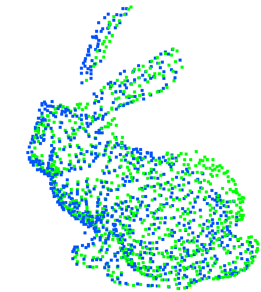
Two specific scans of the “Stanford Bunny” dataset [28] are selected (see Fig. 3), with a relative rotation of about the axis. Each bunny has an average nearest-neighbor (NN) distance of around . The correspondence between source and target points is pre-established using the matching system described in [30]. It suffices to say the point matching is not perfect and hence the number of true correspondence (TCs) and its ratio with respect to the total number of correspondences is .
The performance of the GA-LMS with (selected via extensive parametric simulations) is depicted in Fig. 4. It shows the curve (in blue) for the mean-square error (MSE), which is approximated by the instantaneous squared error (MSE), where is the noise-corrupted version of (in order to model acquisition noise in the scan). As in a real-time online registration, the AF runs only one realization, producing a noisy MSE curve (it is not an ensemble average). Nevertheless, from the cost function (5) curve (in green), plotted on top of the MSE using only the good correspondences, one can see the GA-LMS minimizes it, achieving a steady-state error of at . The PCL SVD-based method achieves a slightly lower error of (see supplementary material), although using all the pairs at each iteration. The GA-LMS uses only 1 pair.

VI Conclusion
This work introduced a new AF completely derived using GA theory. The GA-LMS was shown to be functional when estimating the relative rotation between two PCDs, achieving errors similar to those provided by the SVD-based method used for comparison. The GA-LMS, unlike the SVD method, allows to assess each correspondence pair individually (one pair per iteration). That fact is reflected on the GA-LMS computational cost per iteration – it does not depend on the number of correspondence pairs (points) to be processed, which can lower the computation cost (compared to SVD) of a complete registration algorithm, particularly when grows. To improve performance, some strategies could be adopted: reprocessing iterations in which the MSE changes abruptly, and data reuse techniques [31, 32, 33]. A natural extension is to generalize the method to estimate multivectors of any grade, covering a wider range of applications.
For a general multivector and a unit rotor , it holds that
| (15) |
Proof:
Given that the scalar part (0-grade) of a multivector is not affected by rotation , and using the product rule, one can write
| (16) |
Using the scalar product definition, the cyclic reordering property, and Eq. (7.2) in [23], Plugging back into (16) and multiplying by from the left, . Since the term is an algebraic scalar, . ∎
References
- [1] Paulo S. R. Diniz, Adaptive Filtering: Algorithms and Practical Implementation, Springer US, 4 edition, 2013.
- [2] A.H. Sayed, Adaptive filters, Wiley-IEEE Press, 2008.
- [3] E. Hitzer, “Introduction to Clifford’s Geometric Algebra,” Journal of the Society of Instrument and Control Engineers, vol. 51, no. 4, pp. 338–350, 2012.
- [4] D. Hestenes, New Foundations for Classical Mechanics, Fundamental Theories of Physics. Springer, 1999.
- [5] D. Hestenes and G. Sobczyk, Clifford Algebra to Geometric Calculus: A Unified Language for Mathematics and Physics, Fundamental Theories of Physics. Springer Netherlands, 1987.
- [6] Leo Dorst, Daniel Fontijne, and Stephen Mann, Geometric Algebra for Computer Science: An Object-Oriented Approach to Geometry (The Morgan Kaufmann Series in Computer Graphics), Morgan Kaufmann Publishers Inc., San Francisco, CA, USA, 2007.
- [7] Roxana Bujack, Gerik Scheuermann, and Eckhard Hitzer, “Detection of outer rotations on 3d-vector fields with iterative geometric correlation and its efficiency,” Advances in Applied Clifford Algebras, pp. 1–19, 2013.
- [8] C.J.L. Doran and A.N. Lasenby, Geometric Algebra for Physicists, Cambridge University Press, 2003.
- [9] Chris J. L. Doran, Geometric Algebra and Its Application to Mathematical Physics, Ph.D. thesis, University of Cambridge, 1994.
- [10] Radu Bogdan Rusu and Steve Cousins, “3D is here: Point Cloud Library (PCL),” in IEEE International Conference on Robotics and Automation (ICRA), Shanghai, China, May 9-13 2011.
- [11] Carl D. Meyer, Matrix Analysis and Applied Linear Algebra, SIAM, 2001.
- [12] S. Umeyama, “Least-squares estimation of transformation parameters between two point patterns,” Pattern Analysis and Machine Intelligence, IEEE Transactions on, vol. 13, no. 4, pp. 376–380, Apr 1991.
- [13] Berthold K. P. Horn, “Closed-form solution of absolute orientation using unit quaternions,” Journal of the Optical Society of America A, vol. 4, no. 4, pp. 629–642, 1987.
- [14] G.E. Forsythe and P. Henrici, “The cyclic jacobi method for computing the principal values of a complex matrix,” in Trans. Amer. Math. Soc., Volume 94, Issue 1, Pages 1-23, 1960.
- [15] Michael W. Walker, Lejun Shao, and Richard A. Volz, “Estimating 3-d location parameters using dual number quaternions,” CVGIP: Image Underst., vol. 54, no. 3, pp. 358–367, Oct. 1991.
- [16] P.J. Besl and Neil D. McKay, “A method for registration of 3-d shapes,” Pattern Analysis and Machine Intelligence, IEEE Transactions on, vol. 14, no. 2, pp. 239–256, 1992.
- [17] Zhengyou Zhang, “Iterative point matching for registration of free-form curves and surfaces,” Int. J. Comput. Vision, vol. 13, no. 2, pp. 119–152, Oct. 1994.
- [18] Patrick R. Girard, Quaternions, Clifford Algebras and Relativistic Physics, Birkhäuser Basel, 2007.
- [19] Erik B. Dam, Martin Koch, and Martin Lillholm, “Quaternions, interpolation and animation - diku-tr-98/5,” Tech. Rep., Department of Computer Science, University of Copenhagen, 1998. Available: http://web.mit.edu/2.998/www/QuaternionReport1.pdf.
- [20] D.P. Mandic, C. Jahanchahi, and C.C. Took, “A quaternion gradient operator and its applications,” Signal Processing Letters, IEEE, vol. 18, no. 1, pp. 47–50, Jan 2011.
- [21] C. Jahanchahi, C.C. Took, and D.P. Mandic, “On gradient calculation in quaternion adaptive filtering,” in Acoustics, Speech and Signal Processing (ICASSP), 2012 IEEE International Conference on, March 2012, pp. 3773–3776.
- [22] Mengdi Jiang, Wei Liu, and Yi Li, “A general quaternion-valued gradient operator and its applications to computational fluid dynamics and adaptive beamforming,” in Digital Signal Processing (DSP), 2014 19th International Conference on, Aug 2014, pp. 821–826.
- [23] E. Hitzer, “Multivector differential calculus,” Advances in Applied Clifford Algebras, vol. 12, no. 2, pp. 135–182, 2002.
- [24] C.C. Took and D.P. Mandic, “The quaternion lms algorithm for adaptive filtering of hypercomplex processes,” Signal Processing, IEEE Transactions on, vol. 57, no. 4, pp. 1316–1327, April 2009.
- [25] F.G.A. Neto and V.H. Nascimento, “A novel reduced-complexity widely linear qlms algorithm,” in Statistical Signal Processing Workshop (SSP), 2011 IEEE, June 2011, pp. 81–84.
- [26] E. Hitzer, “Algebraic foundations of split hypercomplex nonlinear adaptive filtering,” Mathematical Methods in the Applied Sciences, vol. 36, no. 9, pp. 1042–1055, 2013.
- [27] J. Lasenby, W. J. Fitzgerald, A. N. Lasenby, and C. J. L. Doran, “New geometric methods for computer vision: An application to structure and motion estimation,” Int. J. Comput. Vision, vol. 26, no. 3, pp. 191–213, Feb. 1998.
- [28] Greg Turk and Marc Levoy, “Zippered polygon meshes from range images,” in Proceedings of the 21st Annual Conference on Computer Graphics and Interactive Techniques, New York, NY, USA, 1994, SIGGRAPH ’94, pp. 311–318, ACM.
- [29] Florian Seybold and U Wössner, “Gaalet-a c++ expression template library for implementing geometric algebra,” in 6th High-End Visualization Workshop, 2010.
- [30] Anas Al-Nuaimi, Martin Piccolorovazzi, Suat Gedikli, Eckehard Steinbach, and Georg Schroth, “Indoor location recognition using shape matching of kinectfusion scans to large-scale indoor point clouds.,” in Eurographics, Workshop on 3D Object Retrieval, 2015.
- [31] W.B. Lopes and C.G. Lopes, “Incremental-cooperative strategies in combination of adaptive filters,” in Int. Conf. in Acoust. Speech and Signal Process. IEEE, 2011, pp. 4132 –4135.
- [32] W.B. Lopes and C.G. Lopes, “Incremental combination of rls and lms adaptive filters in nonstationary scenarios,” in Int. Conf. in Acoust. Speech and Signal Process. IEEE, 2013.
- [33] Luiz F. O. Chamon and Cassio G. Lopes, “There’s plenty of room at the bottom: Incremental combinations of sign-error lms filters.,” in ICASSP, 2014, pp. 7248–7252.