Strong convergence rates for nonlinearity-truncated Euler-type approximations of stochastic
Ginzburg-Landau equations

In this article we study strong numerical approximations of semilinear stochastic evolution equations (SEEs) with superlinearly growing nonlinearities. The explicit Euler scheme and the linear-implicit Euler scheme are known to diverge strongly and numerically weakly in the case of such SEEs; see Theorem 2.1 in Hutzenthaler et al. [19], Theorem 2.1 in Hutzenthaler al. [21], and Section 5.1 in Kurniawan [29]. Fully drift-implicit Euler schemes have been shown to converge strongly even in the case of some SEEs with superlinearly growing nonlinearities and thereby overcome the lack of strong convergence of the explicit and the linear-implicit Euler scheme; see, e.g., Theorem 2.4 in Hu [16], Theorem 2.10 Gyöngy & Millet [11], and Theorem 1.1 in Kovács et al. [26]. Fully drift-implicit Euler schemes can, however, often only be simulated approximatively as a nonlinear equation has to be solved in each time step and the resulting approximations of the fully drift-implicit Euler approximations require additional computational effort (particularly, when the state space of the considered SEE is high dimensional, see, e.g., Figure 4 in Hutzenthaler et al. [20]) and have not yet been shown to converge strongly. Recently, a series of explicit and easily implementable time-discrete approximation schemes have been proposed and shown to converge strongly in the case of SEEs with superlinearly growing nonlinearities; see, e.g., Hutzenthaler et al. [20], Wang & Gan [45], Hutzenthaler & Jentzen [18], Tretyakov & Zhang [44], Halidias [13], Sabanis [39, 40], Halidias & Stamatiou [15], Hutzenthaler et al. [22], Szpruch & Zhāng [42], Halidias [14], Liu & Mao [30], Hutzenthaler & Jentzen [17], Zhang [46], Dareiotis et al. [10], Kumar & Sabanis [27], Beyn et al. [1], Zong et al. [47], Song et al. [41], Ngo & Luong [36], Tambue & Mukam [43], Mao [34], Beyn et al. [2], Kumar & Sabanis [28], and Mao [35] in the case of finite dimensional SEEs and see, e.g., Gyöngy et al. [12] and Jentzen & Pušnik [25] in the case of infinte dimensional SEEs. These schemes are suitable modified versions of the explicit Euler scheme that somehow tame/truncate the superlinearly growing nonlinearities of the considered SEE and thereby prevent the considered tamed scheme from strong divergence. However, each of the above mentioned temporal strong convergence results for implicit (see [16, 11, 26]) and explicit (see [20, 45, 18, 44, 13, 39, 40, 15, 22, 42, 14, 30, 17, 46, 10, 27, 12, 1, 47, 41, 25, 36, 43, 34, 2, 28, 35]) schemes applies merely to trace noise class driven SEEs and excludes the important case of the more irregular space-time white noise. In particular, none of these results applies to space-time white noise driven stochastic Ginzburg-Landau equations. In this work we intend to close this gap and we propose (see (3) and (4) below) and analyze (see Theorem 5.3 below) suitable explicit and strongly convergent approximation schemes for possibly space-time white noise driven SEEs. In particular, we establish essentially sharp strong convergence rates for suitable explicit nonlinearity-truncated approximation schemes for space-time white noise driven stochastic Ginzburg-Landau equations (see (5), Corollary 6.15, and Corollary 6.17 below).

To illustrate the main result of this article (see Theorem 5.3 in Section 5.3 below) in more detail, we consider the following example of our general setting (see Section 5.1) in this introductory section. Let $T\in(0,\infty)$, $n\in\{1,3,5,\ldots\}$, $a_{0},a_{1},\ldots,a_{n-1}\in\mathbb{R}$, $a_{n}\in(-\infty,0)$, $\xi\in H^{2}_{0}((0,1);\mathbb{R})$, $H=L^{2}((0,1);\mathbb{R})$, let $F\colon L^{2n}((0,1);\mathbb{R})\rightarrow H$ be the function with the property that for all $v\in L^{2n}((0,1);\mathbb{R})$ it holds that $F(v)=\sum_{k=0}^{n}a_{k}v^{k}$, let $A\colon D(A)\subseteq H\rightarrow H$ be the Laplacian with Dirichlet boundary conditions on $H$, let $(\Omega,\mathcal{F},\mathbb{P})$ be a probability space with a normal filtration $(\mathcal{F}_{t})_{t\in[0,T]}$, and let $(W_{t})_{t\in[0,T]}$ be an $\textup{Id}_{H}$-cylindrical $(\mathcal{F}_{t})_{t\in[0,T]}$-Wiener process. The assumptions that $n$ is odd and that $a_{n}<0$ ensure that there exists an up to indistinguishability unique $(\mathcal{F}_{t})_{t\in[0,T]}$-adapted stochastic process $X\colon[0,T]\times\Omega\rightarrow L^{2n}((0,1);\mathbb{R})$ with continuous sample paths which satisfies that for all $t\in[0,T]$ it holds $\mathbb{P}$-a.s. that

(cf., e.g., Section 7.2 in Da Prato & Zabczyk [8] and Chapter 6 in Cerrai [4]). The stochastic process $X$ is thus a mild solution of the SPDE

with $X_{0}(x)=\xi(x)$ and $X_{t}(0)=X_{t}(1)=0$ for $x\in(0,1)$, $t\in[0,T]$. In the case $n=3$ and $a_{0}=a_{2}=0$, the SPDE (2) is often referred to as stochastic Ginzburg-Landau equation in the literature (see also (6) below). In this article we introduce the following nonlinearity-truncated exponential scheme to approximate the solution process $X$ of the SPDE (2). Let $\lfloor\cdot\rfloor_{h}\colon\mathbb{R}\rightarrow\mathbb{R}$, $h\in(0,\infty)$, be the mappings with the property that for all $h\in(0,\infty)$, $t\in\mathbb{R}$ it holds that $\lfloor t\rfloor_{h}=\max\!\left(\{0,h,-h,2h,-2h,\ldots\}\cap(-\infty,t]\right)$, let $\chi\in(0,\frac{1}{2n}]$, and let $Y^{N}\colon[0,T]\times\Omega\to L^{2n^{2}}\!((0,1);\mathbb{R})$, $N\in\mathbb{N}$, be stochastic processes which satisfy that for all $t\in[0,T]$, $N\in\mathbb{N}$ it holds $\mathbb{P}$-a.s. that

The approximation scheme (3) is a nonlinearity-truncated modification (cf. (2) in Jentzen & Pušnik [25]) of a time-continuous version (cf., e.g., (130)–(134) in Da Prato et al. [7]) of the classical exponential Euler approximation scheme for semilinear SPDEs (cf., e.g., (3.2) and (3.6) in Lord & Rougemont [31]). We also propose the following nonlinearity-truncated linear-implicit scheme to approximate the solution process $X$ of the SPDE (2). Let $Z^{N}\colon[0,T]\times\Omega\to L^{2n^{2}}\!((0,1);\mathbb{R})$, $N\in\mathbb{N}$, be stochastic processes which satisfy that for all $t\in[0,T]$, $N\in\mathbb{N}$ it holds $\mathbb{P}$-a.s. that

The approximation scheme (4) is a nonlinearity-truncated modification (cf. (2) in Jentzen & Pušnik [25]) of a time-continuous version (cf., e.g., (142)–(146) in Da Prato et al. [7]) of the classical linear-implicit Euler approximation scheme for semilinear SPDEs. Both approximation schemes, (3) and (4), are easy to implement (cf. (7) and (8) below and cf., e.g., also Section 4 in Lord & Tambue [32]). In Corollary 6.15 and Corollary 6.17 below we prove that for all $p\in(0,\infty)$, $\theta\in[0,\nicefrac{{1}}{{4}})$ there exists a real number $C\in\mathbb{R}$ such that for all $N\in\mathbb{N}$ it holds that

Our proofs of (5), Corollary 6.15, and Corollary 6.17, respectively, are based on the well known idea to substract the Ornstein-Uhlenbeck process from the solution process of the SPDE (cf. Section 2 below and, e.g., (14.2.2)–(14.2.3) in Section 14.2 in Da Prato & Zabczyk [9]), are based on some arguments in Jentzen & Kurniawan [24] and Jentzen & Pušnik [25], and are based on an appropriate Lyapunov-type condition for one-step approximation schemes on Banach spaces (see (10) in Section 2.1, (85) in Section 5.1, and Corollary 6.3). To the best of our knowledge, inequality (5), Corollary 6.15, and Corollary 6.17, respectively, are the first results in the literature that establish strong convergence for temporal numerical approximations of the SPDE (2) in the case where $n>1$.

In the following we illustrate (5) through a numerical example. For this we consider the choice $T=1$, $n=3$, $a_{0}=0$, $a_{1}=1$, $a_{2}=0$, $a_{3}=-1$, $\xi=0$, $\chi=\nicefrac{{1}}{{6}}=\nicefrac{{1}}{{2n}}$ and we note that the SPDE (2) reduces in this case to the stochastic Ginzburg-Landau equation

with $X_{0}(x)=0$ and $X_{t}(0)=X_{t}(1)=0$ for $x\in(0,1)$, $t\in[0,T]$. Note that the approximation processes in (3) and (4) satisfy in the case of (6) that for all $n\in\{1,2,\ldots,N-1\}$, $N\in\mathbb{N}$ it holds $\mathbb{P}$-a.s. that $Y_{0}^{N}=Z_{0}^{N}=0$ and

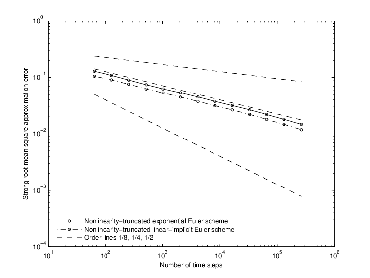
In Figure 1 we plot approximatively the strong root mean square approximation errors

against the number of time steps $N\in\{64,128,256,\ldots,262144\}$. The infinite dimensional Hilbert space $H=L^{2}((0,1);\mathbb{R})$ in (9) is approximated in Figure 1 through the finite dimensional subspace spanned by the first $1024$ eigenfunctions of the Laplacian, the unknown exact solution process $(X_{t})_{t\in[0,T]}$ of (6) is approximated in Figure 1 through a nonlinearity-truncated linear-implicit Crank-Nicolson approximation with $1048576$ time steps, and the expectations in (9) are approximated in Figure 1 by a Monte Carlo approximation with $25$ Monte Carlo runs. Details can be found in Figure 2 in which we present the Matlab code that has been used to create Figure 1. The order lines in Figure 1 correspond to the convergence orders $\nicefrac{{1}}{{8}}$, $\nicefrac{{1}}{{4}}$, and $\nicefrac{{1}}{{2}}$. Figure 1 thus essentially agrees with our strong convergence result (5) which proves that both schemes, (7) and (8), converge in the sense of (9) with order $\nicefrac{{1}}{{4}}-$.

The remainder of this article is organized as follows. In Section 2 the required a priori moments for the nonlinearity-truncated approximation schemes are established, in Section 3 the error analysis is performed in the pathwise sense under the hypothesis of suitable a priori bounds for the approximation processes, and in Section 4 the error analysis is carried out in the strong $L^{p}$-sense under the hypothesis of appropriate a priori moment bounds for the approximation processes. Section 5 combines the results of Section 2 and Section 4 and thereby establishes Theorem 5.3 which is the main result of this article. The analysis in Sections 2–5 is carried out for abstract stochastic evolution equations on separable Banach and Hilbert spaces, respectively. Section 6 then verifies that the assumptions of Theorem 5.3 in Section 5 are satisfied in the case of concrete stochastic partial differential equations of the type (2) and, in particular, establishes Corollary 6.15 and Corollary 6.17.

References

- [1] Beyn, W.-J., Isaak, E., and Kruse, R. Stochastic C-stability and B-consistency of explicit and implicit Euler-type schemes. J. Sci. Comput. (2015), 1–33.
- [2] Beyn, W.-J., Isaak, E., and Kruse, R. Stochastic C-stability and B-consistency of explicit and implicit Milstein-type schemes. arXiv:1512.06905 (2015), 35 pages.
- [3] Blömker, D., and Jentzen, A. Galerkin approximations for the stochastic Burgers equation. SIAM J. Numer. Anal. 51, 1 (2013), 694–715.
- [4] Cerrai, S. Second order PDE’s in finite and infinite dimension, vol. 1762 of Lecture Notes in Mathematics. Springer-Verlag, Berlin, 2001. A probabilistic approach.
- [5] Cox, S., and van Neerven, J. Convergence rates of the splitting scheme for parabolic linear stochastic Cauchy problems. SIAM J. Numer. Anal. 48, 2 (2010), 428–451.
- [6] Cox, S., and van Neerven, J. Pathwise Hölder convergence of the implicit-linear Euler scheme for semi-linear SPDEs with multiplicative noise. Numer. Math. 125, 2 (2013), 259–345.
- [7] Da Prato, G., Jentzen, A., and Roeckner, M. A mild Ito formula for SPDEs. arXiv:1009.3526 (2012), 39 pages.
- [8] Da Prato, G., and Zabczyk, J. Stochastic equations in infinite dimensions, vol. 44 of Encyclopedia of Mathematics and its Applications. Cambridge University Press, Cambridge, 1992.
- [9] Da Prato, G., and Zabczyk, J. Ergodicity for infinite-dimensional systems, vol. 229 of London Mathematical Society Lecture Note Series. Cambridge University Press, Cambridge, 1996.
- [10] Dareiotis, K., Kumar, C., and Sabanis, S. On tamed Euler approximations of SDEs driven by Lévy noise with applications to delay equations. arXiv:1403.0498 (2015), 27 pages.
- [11] Gyöngy, I., and Millet, A. On discretization schemes for stochastic evolution equations. Potential Anal. 23, 2 (2005), 99–134.
- [12] Gyöngy, I., Sabanis, S., and Šiška, D. Convergence of tamed Euler schemes for a class of stochastic evolution equations. arXiv:1308.1796 (2015), 17 pages.
- [13] Halidias, N. A novel approach to construct numerical methods for stochastic differential equations. Numer. Algorithms 66, 1 (2013), 79–87.
- [14] Halidias, N. Construction of positivity preserving numerical schemes for some multidimensional stochastic differential equations. Discrete Contin. Dyn. Syst. Ser. B 20, 1 (2015), 153–160.
- [15] Halidias, N., and Stamatiou, I. S. On the numerical solution of some nonlinear stochastic differential equations using the semi-discrete method. arXiv:1309.3189 (2014), 36 pages.
- [16] Hu, Y. Semi-implicit Euler-Maruyama scheme for stiff stochastic equations. In Stochastic analysis and related topics, V (Silivri, 1994), vol. 38 of Progr. Probab. Birkhäuser Boston, Boston, MA, 1996, pp. 183–202.
- [17] Hutzenthaler, M., and Jentzen, A. On a perturbation theory and on strong convergence rates for stochastic ordinary and partial differential equations with non-globally monotone coefficients. arXiv:1401.0295 (2014), 41 pages.
- [18] Hutzenthaler, M., and Jentzen, A. Numerical approximations of stochastic differential equations with non-globally Lipschitz continuous coefficients. Mem. Amer. Math. Soc. 236, 1112 (2015), v+99.
- [19] Hutzenthaler, M., Jentzen, A., and Kloeden, P. E. Strong and weak divergence in finite time of Euler’s method for stochastic differential equations with non-globally Lipschitz continuous coefficients. Proc. R. Soc. Lond. Ser. A Math. Phys. Eng. Sci. 467 (2011), 1563–1576.
- [20] Hutzenthaler, M., Jentzen, A., and Kloeden, P. E. Strong convergence of an explicit numerical method for SDEs with non-globally Lipschitz continuous coefficients. Ann. Appl. Probab. 22, 4 (2012), 1611–1641.
- [21] Hutzenthaler, M., Jentzen, A., and Kloeden, P. E. Divergence of the multilevel Monte Carlo Euler method for nonlinear stochastic differential equations. Ann. Appl. Probab. 23, 5 (2013), 1913–1966.
- [22] Hutzenthaler, M., Jentzen, A., and Wang, X. Exponential integrability properties of numerical approximation processes for nonlinear stochastic differential equations. arXiv:1309.7657 (2014), 32 pages.
- [23] Jentzen, A. Numerical analysis of stochastic partial differential equations. Lecture notes, ETH Zurich, summer semester 2015, available online at http://www.math.ethz.ch/education/bachelor/lectures/fs2015/math/numsol, May 2015.
- [24] Jentzen, A., and Kurniawan, R. Weak convergence rates for Euler-type approximations of semilinear stochastic evolution equations with nonlinear diffusion coefficients. arXiv:1501.03539 (2015), 51 pages.
- [25] Jentzen, A., and Pušnik, P. Strong convergence rates for an explicit numerical approximation method for stochastic evolution equations with non-globally Lipschitz continuous nonlinearities. arXiv:1504.03523 (2015), 38 pages.
- [26] Kovács, M., Larsson, S., and Lindgren, F. On the discretization in time of the stochastic Allen-Cahn equation. arXiv:1510.03684 (2015), 34 pages.
- [27] Kumar, C., and Sabanis, S. On tamed Milstein schemes of SDEs driven by Lévy noise. arXiv:1407.5347 (2015), 45 pages.
- [28] Kumar, C., and Sabanis, S. On Milstein approximations with varying coefficients: the case of super-linear diffusion coefficients. arXiv:1601.02695 (2016), 31 pages.
- [29] Kurniawan, R. Numerical approximations of stochastic partial differential equations with non-globally Lipschitz continuous nonlinearities. University of Zurich and ETH Zurich, Zurich, Switzerland, 2014. 74 pages. Master thesis.
- [30] Liu, W., and Mao, X. Strong convergence of the stopped Euler-Maruyama method for nonlinear stochastic differential equations. Appl. Math. Comput. 223 (2013), 389 – 400.
- [31] Lord, G. J., and Rougemont, J. A numerical scheme for stochastic PDEs with Gevrey regularity. IMA J. Numer. Anal. 24, 4 (2004), 587–604.
- [32] Lord, G. J., and Tambue, A. Stochastic exponential integrators for the finite element discretization of SPDEs for multiplicative and additive noise. IMA J. Numer. Anal. 33, 2 (2013), 515–543.
- [33] Lunardi, A. Interpolation theory, second ed. Appunti. Scuola Normale Superiore di Pisa (Nuova Serie). [Lecture Notes. Scuola Normale Superiore di Pisa (New Series)]. Edizioni della Normale, Pisa, 2009.
- [34] Mao, X. The truncated Euler-Maruyama method for stochastic differential equations. J. Comput. Appl. Math. 290 (2015), 370 – 384.
- [35] Mao, X. Convergence rates of the truncated Euler-Maruyama method for stochastic differential equations. J. Comput. Appl. Math. 296 (2016), 362 – 375.
- [36] Ngo, H.-L., and Luong, D.-T. Strong rate of tamed Euler-Maruyama approximation for stochastic differential equations with Hölder continuous diffusion coefficient. To appear in Braz. J. Prob. Stat., available online at http://imstat.org/bjps/papers/BJPS301.pdf, August 2015, 18 pages.
- [37] Pazy, A. Semigroups of linear operators and applications to partial differential equations, vol. 44 of Applied Mathematical Sciences. Springer-Verlag, New York, 1983.
- [38] Renardy, M., and Rogers, R. C. An introduction to partial differential equations, second ed., vol. 13 of Texts in Applied Mathematics. Springer-Verlag, New York, 2004.
- [39] Sabanis, S. A note on tamed Euler approximations. Electron. Commun. Probab. 18 (2013), no. 47, 1–10.
- [40] Sabanis, S. Euler approximations with varying coefficients: the case of superlinearly growing diffusion coefficients. arXiv:1308.1796 (2015), 24 pages.
- [41] Song, M. H., Lu, Y. L., and Liu, M. Z. Convergence of the tamed Euler scheme for stochastic differential equations with piecewise continuous arguments under non-Lipschitz continuous coefficients. arXiv:1502.00058 (2015), 16 pages.
- [42] Szpruch, L., and Zhāng, X. -integrability, asymptotic stability and comparison theorem of explicit numerical schemes for SDEs. arXiv:1310.0785 (2015), 33 pages.
- [43] Tambue, A., and Mukam, J. D. Strong convergence of the tamed and the semi-tamed Euler schemes for stochastic differential equations with jumps under non-global Lipschitz condition. arXiv:1510.04729 (2015), 35 pages.
- [44] Tretyakov, M. V., and Zhang, Z. A fundamental mean-square convergence theorem for SDEs with locally Lipschitz coefficients and its applications. SIAM J. Numer. Anal. 51, 6 (2013), 3135–3162.
- [45] Wang, X., and Gan, S. The tamed Milstein method for commutative stochastic differential equations with non-globally Lipschitz continuous coefficients. J. Difference Equ. Appl. 19, 3 (2013), 466–490.
- [46] Zhang, Z. New explicit balanced schemes for SDEs with locally Lipschitz coefficients. arXiv:1402.3708 (2014), 15 pages.
- [47] Zong, X., Wu, F., and Huang, C. Convergence and stability of the semi-tamed Euler scheme for stochastic differential equations with non-Lipschitz continuous coefficients. Appl. Math. Comput. 228 (2014), 240 – 250.