A Schrödinger Cat Living in Two Boxes

Our cQED system includes two 3D cavities, a quasi-planar linear resonator, and a Y-shaped transmon. A single block of high-purity (5N5) aluminum is machined to form a 3D structure that contains both superconducting cavity resonators and also functions as a package for the sapphire chip with deposited Josephson junction. Each of the two cavities can be considered a 3D version of a $\lambda/4$ transmission line resonator between a center stub 3.2 mm in diameter and a cylindrical wall (outer conductor) 9.5 mm in diameter [1]. The heights of the stubs control the resonance frequency, and are about 12.2 mm and 16.3 mm respectively for Alice and Bob. A tunnel (with a maximum width of 5.8 mm and a maximum height of 3.9 mm) is opened from the outside towards the middle wall between the two cavities, creating a three way joint between the tunnel and the two cavities (see photo image, Fig. S1). The whole package is chemically etched by about 80 $\mu$m after machining to improve the surface quality of the cavity resonators [2].

The superconducting transmon is on a 5.5 mm $\times$ 27.5 mm chip, which is diced from a 430 $\mu$m-thick c-plane sapphire wafer after fabrication. The fabrication process uses electron-beam lithography and the standard shadow-mask evaporation of Al/AlOx/Al Josephson junction. The sapphire chip is inserted into the tunnel, with the antenna pads of the transmon slightly intruding into the coaxial cavities to provide mode coupling. The chip is mechanically held at one end with an aluminum clamping structure and indium seal [3].

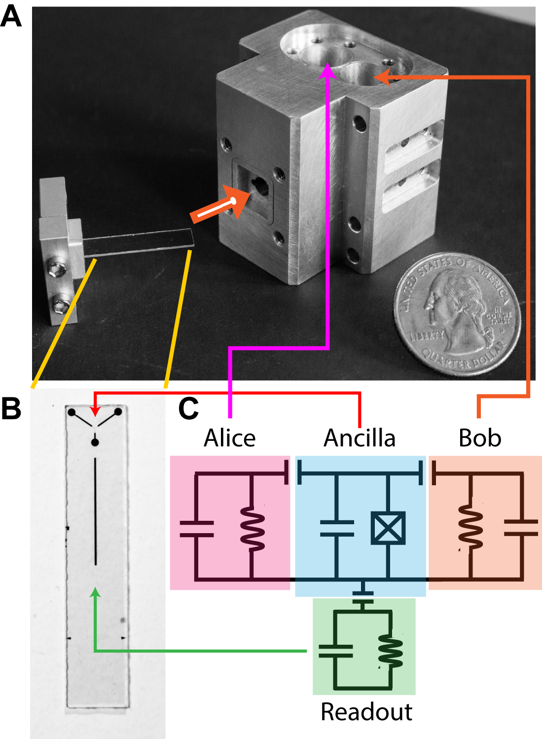
During the transmon fabrication process, a 100 $\mu$m$\times 9.8$ mm strip of aluminum film is also deposited on the sapphire chip. This metal strip and the wall of the tunnel form a planar-3D hybrid $\lambda/2$ stripline resonator. This resonator design has the advantages of both lithographic dimensional control and low surface/radiation loss, and is systematically studied in Ref. [3]. Here it is capacitively coupled to the transmon, and strongly coupled to a 50 $\Omega$ transmission line for readout.

The cQED system has four bosonic modes involved in this experiment: the two 3D cavities, the readout resonator and the transmon ancilla. The transmon can be understood as an LC oscillator with much larger anharmonicity compared with the other modes, and is treated explicitly as a three-level artificial atom. Following Black-box quantization of superconducting circuits [4], the other cavity/resonator modes are modeled as near-harmonic oscillators with weak nonlinearity inherited from coupling to the Josephson junction.

The full system Hamiltonian can then be written in the following form up to the fourth order in the coupling of the resonators to the transmon:

Eq. (S1) is an expanded version of Eq. (3) of the main text, which now includes the readout resonator (with subscript $R$ and operators $r$ and $r^{\dagger}$) as well as Kerr nonlinearities of the cavities. The first two rows represent the excitation energy of the all modes, explicitly including the transmon anharmonicity of $\omega_{ge}-\omega_{ef}=115.17$ MHz. The next three rows are second order terms ($\sim 1$ MHz) representing the dispersive interactions ($\chi$’s) between the transmon and each of the three resonators. The last two rows are the fourth order terms ($\sim 10$ kHz), including the self-Kerr energies ($K_{A},K_{B},K_{R}$) of the resonators and the cross-Kerr interactions between any pairs of resonators ($K_{AB},K_{AR},K_{BR}$). All Hamiltonian parameters of our device are listed in Table S1.

The key Hamiltonian terms that enable the cat state generation and joint parity measurement are the dispersive shifts, $\chi_{A}^{ge},\chi_{A}^{ef},\chi_{B}^{ge},\chi_{B}^{ef}$, highlighted in the main text. Since the readout resonator is always kept in the vacuum state until a final measurement is needed, its Hamiltonian terms do not affect the quantum control and quantum state evolution in this experiment. The fourth-order Hamiltonian terms of Alice and Bob give a minor contribution to the infidelity of the experiment. The self-Kerr terms ($K_{A}$ and $K_{B}$) induce distortion of the Gaussian probability distribution of the coherent state components of the cat state, and will cause state collapse and revival at long time scales [5]. The cross-Kerr interaction $K_{AB}$ induces spontaneous entTrueanglement between Alice and Bob over long time scales in ways not included in our simple analysis.

Fig. S2 shows the diagram of our measurement setup. The device package is installed inside a Cryoperm magnetic shield and thermalized to the mixing chamber of a dilution refrigerator with a base temperature of 20 mK. Low-pass filters and infrared (eccosorb) filters are used to reduce stray radiation and photon shot noise. A Josephson parametric converter (JPC) is also mounted to the 20 mK stage, connected to the output port of the device package via circulators, providing near-quantum-limited amplification, with a power gain of 20dB and bandwidth of 5MHz.

We use a field programmable gate array (FPGA) to operate both the quantum-control pulse sequences and the data acquisition process. Our experiment does not rely on the real-time feedback capability of the FPGA, but our in-house programmed FPGA offers an important practical advantage in its ability to compute rather than store sideband-modulation waveforms. This leads to minimal usage of waveform memory for a large number of different cavity displacements, allowing us to measure the joint Wigner function over a large number of points in the phase space in a single run.

Both cavity drives and transmon drives are generated by sideband-modulation of continuous-wave (CW) carrier tones produced by respective microwave generators. The 4 FPGA analogue channels are used as 2 IQ-pairs that control the cavity drives to implement arbitrary cavity displacements. Rotations of the transmon ancilla are controlled by another pair of IQ channels provided by an arbitrary waveform generator (AWG) synchronized to the FPGA via a digital marker. This IQ pair controls both $|g\rangle$-$|e\rangle$ and $|e\rangle$-$|f\rangle$ transitions by using different intermediate frequencies (IF).

Ancilla readout is performed by heterodyne measurement of the microwave transmission of a readout pulse through the two ports of the quasi-planar readout resonator near its resonance frequency. Using the well-established cQED dispersive readout [6], the amplitude and phase of the transmitted signal depends on the quantum state of the ancilla. This readout pulse is produced by a microwave generator (RO) gated by a FPGA digital channel. The transmitted signal, after being amplified by the JPC, is further amplified by a high electron mobility transistor (HEMT) at 4K and a regular RF amplifier at room temperature. The amplified signal is then mixed down to 50 MHz with the output of a “local oscillator” (LO) microwave generator, and analyzed by the FPGA. A split copy of the readout pulse is directly mixed with the LO without entering the refrigerator to provide a phase reference for the measured transmission.

The long lifetimes of the cavities allow preparation of highly coherent cavity quantum states, but severely limits the rate one can repeat the measurement process. (With $T_{1}\approx 3$ ms for Alice, it takes 15-20 ms for the cavity photon number to naturally decay to the order of 0.01.) Since tomographic measurement of the two-cavity quantum state requires large amounts of measurements, we implement four-wave mixing processes to realize fast reset for both cavities[7]. These processes effectively convert photons in Alice or Bob into photons in the short-lived readout resonator mode using three parametric pumping tones. We apply this reset operation for 400 $\mu$s, and acquire our experimental data with a repetition cycle of about 900 $\mu$s.

Ideally, in thermal equilibrium at our base temperature (20 mK) all modes (Alice, Bob, or ancilla) of our quantum system should be in their ground state. However, in our experiment there is a non-negligible probability that any of the three modes is found in an excited state possibly due to insufficient thermalization. These erroneous excited state populations, about 8$\%$ for the ancilla and 2-3$\%$ for Alice and Bob, can reduce the fidelity of the subsequently-prepared quantum state and the parity measurement. To eliminate these effects, we perform two measurements as shown in Fig. S3 to “purify” the initial state of the system before we start each run of the experiment. This is implemented by post-selecting the cases where our experiment starts from the ground state, $|g\rangle|0\rangle_{A}|0\rangle_{B}$, before any non-trivial quantum operation is performed, which amounts to about 80% of the all the data acquired. It should be noted that the use of post-selection here is purely for experimental convenience and does not compromise the deterministic nature of the generation of cat states. One can in principle use real-time feedback to prepare the initial state and achieve a slightly higher data rate. No post-selection beyond the ground state initialization is applied in our analyses of the two-mode cat state.

The Hamiltonian parameters and coherence properties of the device are mostly characterized by adapting established techniques, in particular, various forms of Ramsey interferometry. The measured coherence times of the Alice, Bob and the ancilla are listed in Table I of the main text, and a more complete list is provided in Table S2. We briefly comment on a few characterization methods that are noteworthy.

Measurement of the coherence of higher excited states of a superconducting transmon is a relatively new topic recently reported in Ref. [8]. In addition to using a similar sequence to determine $T_{2,ef}^{*}$ between $|f\rangle$ and $|e\rangle$, we note that $T_{2,gf}^{*}$ (between $|f\rangle$ and $|g\rangle$) is more relevant to our experiment. This $T_{2,gf}^{*}$ time cannot be simply derived from $T_{2,ge}^{*}$ and $T_{2,ef}^{*}$, but can be determined by a Ramsey experiment starting from a $\frac{1}{\sqrt{2}}(|g\rangle+|f\rangle)$ superposition.

The coherence times of Alice and Bob are measured using Ramsey interference of $|0\rangle$ and $|1\rangle$ Fock states following a Selective Number Arbitrary Phase (SNAP) gate [9] that prepares the Fock state superposition. This method, which is described in Ref. [1], extracts the $T_{2}^{*}$ without being affected by high-order nonlinearities (Fig. S4). Together with the measurement of the cavity $T_{1}$, we find the cavity pure dephasing time $T_{\phi}=1/(\frac{1}{T_{2}^{*}}-\frac{1}{2T_{1}})=1.1\pm 0.2$ ms for Alice and $0.9\pm 0.2$ ms for Bob. Such pure dephasing times can be fully explained by their dispersive frequency shifts due to the thermal excitation of the transmon ancilla [1]. The rate of the $|g\rangle\rightarrow|e\rangle$ transition of the transmon, $\Gamma_{\uparrow}$, can be determined from its $T_{1}$ and thermal population of the $|e\rangle$ state, $P_{e}$: $\Gamma_{\uparrow}=P_{e}/T_{1}=7.5\%/(70$ $\mu\rm{s})=1/(0.9$ ms). In addition, the cavity Ramsey experiment also allows extraction of the precise resonance frequency of the cavity. Over the course of 8 months while the device was continuously operated at 20 mK, we observed no slow drift of cavity frequency exceeding its linewidth ($\approx 200$ Hz).

The dispersive frequency shifts ($\chi$’s) are measured both in the frequency domain by spectroscopy techniques and in the time domain by a Ramsey-type qubit state revival experiment [10]) (Fig. S5). These techniques established previously for 2-level qubits, can both be extended for the 3-level artificial atom considered in this study. The latter measurement is also a valuable procedure for tuning up the joint parity measurement.

The self-Kerr effect of Alice or Bob ($K_{A}$ or $K_{B}$ terms in the Hamiltonian) can be characterized by the collapse and revival of a single-cavity coherent state [5]. In addition, with two long-lived cavities, we are able to directly measure the inter-cavity cross-Kerr effect ($K_{AB}$) by observing the frequency shift of Bob in response to the presence of photons in Alice.

The two-mode cat state is generated deterministically using conditional operations between the ancilla and the two cavities. As presented in the main text (Fig. 1C), the generation sequence is composed of the following steps [11]: 1) preparing ancilla superposition ($R^{ge}_{\pi/2}$), 2) displacements of Alice and Bob conditional on the ancilla state ($D^{g}_{2\alpha}$), realizing a three-way entangling gate, 3) conditional flip (reset) of ancilla ($R^{00}_{\pi}$), disentangling it from the cavity state, 4) unconditional displacements of Alice and Bob ($D_{-\alpha}$) to center the cat state in the phase space (which is a trivial step purely for convenience of presentation).

The conditional displacement ($D^{g}_{2\alpha}$) is the key step in this state generation process. Although this operation can be directly implemented using cavity drives with a bandwidth smaller than the dispersive interaction strength ($\chi^{ge}_{i}$, $i$=A or B), such a method requires a rather long pulse duration (and therefore higher infidelity due to decoherence and Kerr effects). Alternatively, for each cavity we use two unconditional displacements separated by a wait time $\Delta t$ in between to effectively realize $D^{g}_{2\alpha}$.

During the wait time $\Delta t$, due to the dispersive interaction, cavity coherent states in both cavities accumulate conditional phases of $\phi_{i}=\chi^{ge}_{i}\Delta t$ if the ancilla is in $|e\rangle$:

Using the IQ plane to describe the photon probability distribution in each cavity in the rotating frame, a coherent state $|\alpha^{\prime}\rangle_{i}$ can be represented by a (Gaussian) circle that stays stationary when the ancilla is in $|g\rangle$, and rotates with the angular velocity $\chi^{ge}_{i}$ when the ancilla is in $|e\rangle$: $|\alpha^{\prime}\rangle_{i}\rightarrow|\alpha^{\prime}e^{i\chi_{i}^{ge}\Delta t}\rangle_{i}$. Therefore, this conditional phase gate can split the cavity coherent state in phase space when the ancilla is prepared in $\frac{1}{\sqrt{2}}(|g\rangle+|e\rangle)$, effectively realizing a conditional displacement. A similar strategy has been previously implemented for a single cavity [10]. The actual pulse sequences for creating the two-mode cat state and the resultant state evolution for the two cavity system are illustrated in Fig. S6.

In this work we have focused on studying the two-mode cat state $|\psi_{\pm}\rangle$. This state is equivalent to a cat state of the form $\mathcal{N}(|\sqrt{2}\alpha\rangle_{C}\pm|-\sqrt{2}\alpha\rangle_{C})$ in a hybridized mode basis of $c^{\dagger}=\frac{1}{\sqrt{2}}(a^{\dagger}+b^{\dagger})$. Cat-state control over the $c^{\dagger}$ mode alone would not be fundamentally more useful than controlling a single local mode (as in previous works) if we cannot access modes other than $c^{\dagger}$. However, it is easy to see that we can create cat states in Alice (or Bob) alone by omitting all pulses on Bob (or Alice) in Fig. S6. The resultant conventional single-mode cat state can be characterized by Wigner tomography of individual cavities (Fig. S7). Furthermore, we can reverse the cavity displacements in either Alice or Bob in Fig. S6 to realize a cat state in the $\frac{1}{\sqrt{2}}(a^{\dagger}-b^{\dagger})$ basis. The important message from the present experiment is that we can create cat states in an arbitrary basis spanned by two modes. In fact, it can be shown that the dispersive Hamiltonian permits universal quantum control of this system. [12] [13]

Measurement of the joint photon number parity, $P_{J}$, is critical to our study of two-cavity quantum states. Here we explain in detail the quantum operations and required system parameters to realize such measurements.

Photon parity measurement of a single-cavity quantum state using an ancilla qubit (using only $|g\rangle$ and $|e\rangle$ levels) has been previous demonstrated in Ref. [14] (see Fig. 1 therein). This single-cavity protocol is applicable to either one of our cavities when the other cavity is in the vacuum state. It uses the dispersive interaction $\chi^{ge}_{i}$ to map even-photon-number and odd-photon-number states in the cavity of interest (i=A or B) to different qubit levels. This is realized by two $\pi/2$ rotations of the qubit, $R^{ge}_{\pi/2}$ (around the same X-axis), separated by a wait time of $\pi/\chi^{ge}_{i}$. For example, if Bob is in the vacuum state ($b^{\dagger}b=0$), the conditional phase shift described in Eq. (S2) over the time $\Delta t=\pi/\chi^{ge}_{A}$ is:

This is equivalent to a qubit Z-rotation of $\pi$ conditioned on the photon number in Alice being odd because $e^{i\pi a^{\dagger}a}=P_{A}$. Therefore the whole sequence $R^{ge}_{\pi/2}C^{A}_{\pi}R^{ge}_{\pi/2}$ flips the qubit if and only if the photon number parity in Alice is even, and subsequent readout of the qubit state measures the parity.

The control and measurement sequence described above can in principle be directly implemented in our experiment to measure the joint photon number parity if $\chi_{A}^{ge}$ is exactly equal to $\chi_{B}^{ge}$. This is because for a wait time of $\Delta t=\pi/\chi_{A}^{ge}(=\pi/\chi_{B}^{ge})$, from Eq. (S2) we have:

Noting $P_{J}=P_{A}P_{B}$, an identical control sequence of $R^{ge}_{\pi/2}U(\Delta t)R^{ge}_{\pi/2}$ followed by a qubit readout would achieve the joint parity measurement. However, without strictly identical $\chi_{A}^{ge}$ and $\chi_{B}^{ge}$, the phase accumulation in one cavity is faster than the other, and it is in general not possible to realize parity operators in both cavities simultaneously using this simple protocol. Moreover, for a general two-cavity quantum state, this sequence can not measure a single-cavity parity operator ($P_{A}$ or $P_{B}$) due to inevitable entanglement between the ancilla and the photons in the other cavity during the process.

As noted in the main text, we introduce a technique for measuring $P_{J}$ with less stringent requirements on Hamiltonian parameters by exploiting the $|f\rangle$-level of the ancilla. This method is most helpful when the $|e\rangle\rightarrow|g\rangle$ transition of the ancilla shows stronger interaction with Bob ($\chi_{B}^{ge}>\chi_{A}^{ge}$), while the $|f\rangle\rightarrow|e\rangle$ transition shows stronger interaction with Alice ($\chi_{A}^{ef}>\chi_{B}^{ef}$). This is physically realized by engineering the ancilla frequency to lie between the two cavities, i.e.$\omega_{A}<\omega_{ef}<\omega_{ge}<\omega_{B}$.

Considering the quantum state with two cavities and three ancilla levels in general, the unitary evolution for any wait time $\Delta t$ is:

where

Here we define $\chi_{A}^{gf}\equiv\chi_{A}^{ge}+\chi_{A}^{ef}$ and $\chi_{B}^{gf}\equiv\chi_{B}^{ge}+\chi_{B}^{ef}$. Therefore, the two cavities simultaneously acquire conditional phases in their coherent state components at relative rates that differ for $|e\rangle$ and $|f\rangle$.

One possible pulse sequence for such $P_{J}$ measurement using three ancilla levels is shown in Fig. 1C of the main text and reproduced as Fig. S18A. For a given two-cavity quantum state $\Psi_{AB}$, We first use a $R_{\pi/2}^{ge}$ rotation to prepare the ancilla in $\frac{1}{\sqrt{2}}(|g\rangle+|e\rangle)$. Then a wait time $\Delta t_{1}$ imparts phases $\phi_{A1}=\chi_{A}^{ge}\Delta t_{1}$ and $\phi_{B1}=\chi_{B}^{ge}\Delta t_{1}$ to the two cavities for the $|e\rangle$ component of the state:

Next, the $|e\rangle$ component in this intermediate state is converted to $|f\rangle$ by a $\pi$ rotation in the $|e\rangle$-$|f\rangle$ space, $R_{\pi}^{ef}$. Subsequently a second wait time $\Delta t_{2}$ leads to a second simultaneous conditional phase gate, imparting phases $\phi_{A2}=\chi_{A}^{gf}\Delta t_{2}$ and $\phi_{B2}=\chi_{B}^{gf}\Delta t_{2}$ to the two cavities for the now $|f\rangle$ component of the state:

The $|f\rangle$ component is then converted back to $|e\rangle$ by another $R_{\pi}^{ef}$ pulse. If we can find $\Delta t_{1}$ and $\Delta t_{2}$ so that:

the obtained quantum state is:

effectively realizing the simultaneous controlled $\pi$-phase gate ($C^{A}_{\pi}C^{B}_{\pi}$) in Eq. (S4). Finally a $R_{\pi/2}^{ge}$ pulse completes the projection of joint parity to the ancilla $|g\rangle$, $|e\rangle$ levels, ready for readout through the readout resonator.

The condition for finding non-negative solutions for $\Delta t_{1}$ and $\Delta t_{2}$ in Eq. (S9) is that $\chi_{A}^{ge}-\chi_{B}^{ge}$ and $\chi_{A}^{gf}-\chi_{B}^{gf}$ have opposite signs. In essence, the cavity that acquires phase slower than the other at $|e\rangle$ due to smaller $\chi_{i}^{ge}$ is allowed to catch up at $|f\rangle$ using its larger $\chi_{i}^{gf}$.

It should be noted that such relative relation of the $\chi$’s is just a practically preferred condition rather than an absolute mathematical requirement. This is because parity mapping can be achieved whenever both cavities acquire a conditional phase of $\pi$ modulo $2\pi$. It is always possible to allow extra multiples of $2\pi$ phases applied to the cavity with stronger dispersive coupling to the ancilla, although it increases the total gate time and incurs more decoherence. The essential ingredient in engineering the $P_{J}$ operator is the extra tuning parameter $\Delta t_{2}$ (in addition to $\Delta t_{1}$) that allows two equations such as Eq. (S9) to be simultaneously satisfied.

This extra degree of freedom also enables measurement of the photon number parity of a single cavity, $P_{A}$ or $P_{B}$, for an arbitrary two-cavity quantum state. This can be realized with the same control sequences (Fig. S18A), choosing wait times such that one cavity acquires a conditional $\pi$ phase (modulo 2$\pi$) while the other acquires 0 phase (modulo 2$\pi$). For example, to measure $P_{A}$ we use $\Delta t_{1}$ and $\Delta t_{2}$ satisfying:

Fig. S18B shows an alternative version of joint parity mapping protocol, which uses more ancilla operations, but is better adapted to to a larger parameter space of $\chi$’s. In this protocol, the ancilla spends time at the $|e\rangle$-$|f\rangle$ superposition so that conditional phases proportional to $\chi_{i}^{ef}$ are applied to the cavities. To achieve joint parity mapping, the two time intervals $\Delta t_{1}$ and $\Delta t_{2}$ should satisfy:

which can avoid the use of extra $2\pi$ phases to $\chi_{A}^{ef}-\chi_{B}^{ef}$ has opposite sign versus $\chi_{A}^{gf}-\chi_{B}^{gf}$.

Experimentally, choices of the parity mapping sequence and gate times involve trade-offs in various aspects such as pulse speed/bandwidth and coherence time. We have measured joint parity (and subsequently Wigner functions) using both protocols. For the sequence of Fig. S18A, $\Delta t_{1}=0$, $\Delta t_{2}=184$ ns was experimentally implemented. For the sequence of Fig. S18B, $\Delta t_{1}=28$ ns, $\Delta t_{2}=168$ ns was used. The actual effective wait time was longer due to the non-zero duration (16 ns) of each ancilla rotation. The first protocol, with this choice of wait times, does not yield the exact $\pi$ phases required for exact parity mapping (We estimate $\phi_{A1}+\phi_{A2}=0.97\pi$ and $\phi_{B1}+\phi_{B2}=1.03\pi$. These phase errors lead to an estimated infidelity of the joint parity measurement of about 3% for the two-cavity states in this study (Fig. S9). Exact phases can be achieved with longer wait times so that $\phi_{A1}+\phi_{A2}=3\pi$ and $\phi_{B1}+\phi_{B2}=5\pi$, but the infidelity due to decoherence and high-order Hamiltonian terms outweighs the benefits. In principle, the second protocol that achieves exact $\pi$ phases at relatively short total gate time should be more advantageous. However, using the second protocol, we observe visibly identical results of joint Wigner tomography of the two-mode cat states with fidelity nearly equal to the first protocol (Fig. S10). This is attributed to the extra infidelity from the more complicated ancilla rotations involved in the second protocol (due to pulse bandwidth limitations and unwanted ancilla population mixing, see Section .12 of this Supplementary). All joint Wigner tomography shown in the main text are measured using the first protocol (matching Fig. 1C).

Single cavity Wigner tomography is also performed using the protocol of Fig. S18A, with $\Delta t_{1}=688$ ns, $\Delta t_{2}=0$ for $P_{A}$, and $\Delta t_{1}=660$ ns, $\Delta t_{2}=204$ ns for $P_{B}$. Moreover, for $P_{A}$ measurement the $R^{ef}_{\pi}$ pulses were skipped, taking advantage of the fact that $\chi_{B}^{ge}\approx 2\chi_{A}^{ge}$.

The joint tomography of a two-cavity quantum state is described by a four dimensional joint Wigner function $W_{J}(\beta_{A},\beta_{B})$. The most informative plane cuts of $W_{J}$, along Re$(\beta_{A})$-Re$(\beta_{B})$ and Im$(\beta_{A})$-Im$(\beta_{B})$, have been presented in the main text. This section provides additional data of our measurement on the joint quantum state of Alice and Bob.

Fig. S11 shows the joint Wigner function of $|\psi_{+}\rangle$ ($\alpha=1.92$) measured in the natural single-cavity IQ planes, or plane cuts of $W_{J}$ along Re$(\beta_{A})$-Im$(\beta_{A})$ and Re$(\beta_{B})$-Im$(\beta_{B})$ respectively (and through the origin). Both plane cuts contain interference fringes along the imaginary axis as expected. No features of Gaussian coherent states are observed in either figure because the underlying coherent states $|\alpha\rangle_{A}$$|\alpha\rangle_{B}$ and $|-\alpha\rangle_{A}$$|-\alpha\rangle_{B}$ are located outside these plane cuts.

To assist visualization of the two-mode cat state, the joint Wigner function of $|\psi_{-}\rangle$ ($\alpha=1.92$) is further presented as a movie, which is a direct extension of Fig. 3 of the main text. It shows 21 frames of Re$(\beta_{A})$-Re$(\beta_{B})$ plane cuts as a function of the Im$(\beta_{A})$,Im$(\beta_{B})$ coordinates.

References

- [1] S. Haroche, Reviews of Modern Physics 85, 1083 (2013).
- [2] D. J. Wineland, Reviews of Modern Physics 85, 1103 (2013).
- [3] A. Ourjoumtsev, H. Jeong, R. Tualle-Brouri, and P. Grangier, Nature 448, 784 (2007).
- [4] M. Brune, E. Hagley, J. Dreyer, X. Maître, A. Maali, C. Wunderlich, J. M. Raimond, and S. Haroche, Physical Review Letters 77, 4887 (1996).
- [5] B. Vlastakis, G. Kirchmair, Z. Leghtas, S. E. Nigg, L. Frunzio, S. M. Girvin, M. Mirrahimi, M. H. Devoret, and R. J. Schoelkopf, Science 342, 607 (2013).
- [6] I. L. Chuang, D. W. Leung, and Y. Yamamoto, Physical Review A 56, 1114 (1997).
- [7] M. Mirrahimi, Z. Leghtas, V. V. Albert, S. Touzard, R. J. Schoelkopf, L. Jiang, and M. H. Devoret, New Journal of Physics 16, 045014 (2014).
- [8] N. Ofek, A. Petrenko, R. W. Heeres, P. Reinhold, Z. Leghtas, B. Vlastakis, Y. Liu, L. Frunzio, S. M. Girvin, L. Jiang, M. Mirrahimi, M. H. Devoret, and R. J. Schoelkopf, in preparation (2016).
- [9] T. Monz, P. Schindler, J. T. Barreiro, M. Chwalla, D. Nigg, W. A. Coish, M. Harlander, W. Hänsel, M. Hennrich, and R. Blatt, Physical Review Letters 106, 130506 (2011).
- [10] J. Kelly, R. Barends, A. G. Fowler, A. Megrant, E. Jeffrey, T. C. White, D. Sank, J. Y. Mutus, B. Campbell, Y. Chen, Z. Chen, B. Chiaro, A. Dunsworth, I.-C. Hoi, C. Neill, P. J. J. O’Malley, C. Quintana, P. Roushan, A. Vainsencher, J. Wenner, A. N. Cleland, and J. M. Martinis, Nature 519, 66 (2015).
- [11] L. Davidovich, A. Maali, M. Brune, J. M. Raimond, and S. Haroche, Physical Review Letters 71, 2360 (1993).
- [12] A. Ourjoumtsev, F. Ferreyrol, R. Tualle-Brouri, and P. Grangier, Nature Physics 5, 189 (2009).
- [13] B. C. Sanders, Journal of Physics A: Mathematical and Theoretical 45, 244002 (2012).
- [14] P. Milman, A. Auffeves, F. Yamaguchi, M. Brune, J. M. Raimond, and S. Haroche, The European Physical Journal D - Atomic, Molecular, Optical and Plasma Physics 32, 233 (2005).
- [15] H. Paik, D. I. Schuster, L. S. Bishop, G. Kirchmair, G. Catelani, A. P. Sears, B. R. Johnson, M. J. Reagor, L. Frunzio, L. I. Glazman, S. M. Girvin, M. H. Devoret, and R. J. Schoelkopf, Physical Review Letters 107, 240501 (2011).
- [16] See, Supplementary materials for additional information.
- [17] M. Reagor, W. Pfaff, C. Axline, R. W. Heeres, N. Ofek, K. Sliwa, E. Holland, C. Wang, J. Blumoff, K. Chou, M. J. Hatridge, L. Frunzio, M. H. Devoret, L. Jiang, and R. J. Schoelkopf, arXiv:1508.05882 [cond-mat, physics:quant-ph] (2015).
- [18] M. Michael, M. Silveri, R. T. Brierley, V. V. Albert, J. Salmilehto, L. Jiang, and S. M. Girvin, in preparation (2016).
- [19] Z. Leghtas, G. Kirchmair, B. Vlastakis, M. H. Devoret, R. J. Schoelkopf, and M. Mirrahimi, Physical Review A 87, 042315 (2013).
- [20] P. Bertet, A. Auffeves, P. Maioli, S. Osnaghi, T. Meunier, M. Brune, J. M. Raimond, and S. Haroche, Physical Review Letters 89, 200402 (2002).
- [21] L. Sun, A. Petrenko, Z. Leghtas, B. Vlastakis, G. Kirchmair, K. M. Sliwa, A. Narla, M. Hatridge, S. Shankar, J. Blumoff, L. Frunzio, M. Mirrahimi, M. H. Devoret, and R. J. Schoelkopf, Nature 511, 444 (2014).
- [22] S. Deléglise, I. Dotsenko, C. Sayrin, J. Bernu, M. Brune, J.-M. Raimond, and S. Haroche, Nature 455, 510 (2008).
- [23] K. E. Cahill and R. J. Glauber, Physical Review 177, 1882 (1969).
- [24] R. W. Andrews, A. P. Reed, K. Cicak, J. D. Teufel, and K. W. Lehnert, Nature Communications 6, 10021 (2015).
- [25] Z. Y. Ou, S. F. Pereira, H. J. Kimble, and K. C. Peng, Physical Review Letters 68, 3663 (1992).
- [26] B. Julsgaard, A. Kozhekin, and E. S. Polzik, Nature 413, 400 (2001).
- [27] C. Eichler, D. Bozyigit, C. Lang, M. Baur, L. Steffen, J. M. Fink, S. Filipp, and A. Wallraff, Physical Review Letters 107, 113601 (2011).
- [28] E. Flurin, N. Roch, F. Mallet, M. H. Devoret, and B. Huard, Physical Review Letters 109, 183901 (2012).
- [29] I. Afek, O. Ambar, and Y. Silberberg, Science 328, 879 (2010).
- [30] H. Wang, M. Mariantoni, R. C. Bialczak, M. Lenander, E. Lucero, M. Neeley, A. D. O’Connell, D. Sank, M. Weides, J. Wenner, T. Yamamoto, Y. Yin, J. Zhao, J. M. Martinis, and A. N. Cleland, Physical Review Letters 106, 060401 (2011).
- [31] N. Khaneja, T. Reiss, C. Kehlet, T. Schulte-Herbrüggen, and S. J. Glaser, Journal of Magnetic Resonance 172, 296 (2005).
- [32] P. T. Cochrane, G. J. Milburn, and W. J. Munro, Physical Review A 59, 2631 (1999).
- [33] S. T. Flammia and Y.-K. Liu, Physical Review Letters 106, 230501 (2011).
- [34] J. Joo, W. J. Munro, and T. P. Spiller, Physical Review Letters 107, 083601 (2011).
- [35] S. J. van Enk and O. Hirota, Physical Review A 64, 022313 (2001).
- [36] A. Roy, L. Jiang, A. D. Stone, and M. Devoret, Physical Review Letters 115, 150503 (2015).
Supplementary Material:
- [1] M. Reagor, W. Pfaff, C. Axline, R. W. Heeres, N. Ofek, K. Sliwa, E. Holland, C. Wang, J. Blumoff, K. Chou, M. J. Hatridge, L. Frunzio, M. H. Devoret, L. Jiang, and R. J. Schoelkopf, arXiv:1508.05882 [cond-mat, physics:quant-ph] (2015).
- [2] M. Reagor, H. Paik, G. Catelani, L. Sun, C. Axline, E. Holland, I. M. Pop, N. A. Masluk, T. Brecht, L. Frunzio, M. H. Devoret, L. Glazman, and R. J. Schoelkopf, Applied Physics Letters 102, 192604 (2013).
- [3] C. Axline, M. Reagor, P. Reinhold, R. Heeres, C. Wang, W. Pfaff, Y. Chu, L. Frunzio, and R. Schoelkopf, In preparation (2016).
- [4] S. E. Nigg, H. Paik, B. Vlastakis, G. Kirchmair, S. Shankar, L. Frunzio, M. H. Devoret, R. J. Schoelkopf, and S. M. Girvin, Physical Review Letters 108, 240502 (2012).
- [5] G. Kirchmair, B. Vlastakis, Z. Leghtas, S. E. Nigg, H. Paik, E. Ginossar, M. Mirrahimi, L. Frunzio, S. M. Girvin, and R. J. Schoelkopf, Nature 495, 205 (2013).
- [6] A. Wallraff, D. I. Schuster, A. Blais, L. Frunzio, R.-S. Huang, J. Majer, S. Kumar, S. M. Girvin, and R. J. Schoelkopf, Nature 431, 162 (2004).
- [7] Z. Leghtas, T. Touzard, A. Petrenko, I. Pop, A. Kou, B. Vlastakis, A. Narla, K. Sliwa, S. Shankar, M. Hatridge, V. Albert, L. Jiang, L. Frunzio, R. Schoelkopf, M. Mirrahimi, and M. Devoret, In preparation (2016).
- [8] M. J. Peterer, S. J. Bader, X. Jin, F. Yan, A. Kamal, T. J. Gudmundsen, P. J. Leek, T. P. Orlando, W. D. Oliver, and S. Gustavsson, Physical Review Letters 114, 010501 (2015).
- [9] R. W. Heeres, B. Vlastakis, E. Holland, S. Krastanov, V. V. Albert, L. Frunzio, L. Jiang, and R. J. Schoelkopf, Physical Review Letters 115, 137002 (2015).
- [10] B. Vlastakis, G. Kirchmair, Z. Leghtas, S. E. Nigg, L. Frunzio, S. M. Girvin, M. Mirrahimi, M. H. Devoret, and R. J. Schoelkopf, Science 342, 607 (2013).
- [11] Z. Leghtas, G. Kirchmair, B. Vlastakis, M. H. Devoret, R. J. Schoelkopf, and M. Mirrahimi, Physical Review A 87, 042315 (2013).
- [12] I. Chuang, D. W. Leung, and Y. Yamamoto, Physical Review A 56 (1997).
- [13] M. Michael, M. Silveri, R. Brierley, V. V. Albert, J. Salmilehto, L. Jiang, and S. M. Girvin, In preparation (2016).
- [14] L. Sun, A. Petrenko, Z. Leghtas, B. Vlastakis, G. Kirchmair, K. M. Sliwa, A. Narla, M. Hatridge, S. Shankar, J. Blumoff, L. Frunzio, M. Mirrahimi, M. H. Devoret, and R. J. Schoelkopf, Nature 511, 444 (2014).
- [15] N. Khaneja, T. Reiss, C. Kehlet, T. Schulte-Herbrüggen, and S. J. Glaser, Journal of Magnetic Resonance 172, 296 (2005).
- [16] U. Leonhardt, Measuring the Quantum State of Light (Cambridge University Press, 1997).
- [17] C. Rigetti, J. M. Gambetta, S. Poletto, B. L. T. Plourde, J. M. Chow, A. D. Córcoles, J. A. Smolin, S. T. Merkel, J. R. Rozen, G. A. Keefe, M. B. Rothwell, M. B. Ketchen, and M. Steffen, Physical Review B 86, 100506 (2012).
- [18] M. Mirrahimi, Z. Leghtas, V. V. Albert, S. Touzard, R. J. Schoelkopf, L. Jiang, and M. H. Devoret, New Journal of Physics 16, 045014 (2014).
- [19] F. Motzoi, J. M. Gambetta, P. Rebentrost, and F. K. Wilhelm, Physical Review Letters 103, 110501 (2009).
- [20] Z. Chen, J. Kelly, C. Quintana, R. Barends, B. Campbell, Y. Chen, B. Chiaro, A. Dunsworth, A. Fowler, E. Lucero, E. Jeffrey, A. Megrant, J. Mutus, M. Neeley, C. Neill, P. O’Malley, P. Roushan, D. Sank, A. Vainsencher, J. Wenner, T. White, A. Korotkov, and J. M. Martinis, Physical Review Letters 116, 020501 (2016).
- [21] K. Banaszek and K. Wódkiewicz, Physical Review Letters 82, 2009 (1999).
- [22] P. Milman, A. Auffeves, F. Yamaguchi, M. Brune, J. M. Raimond, and S. Haroche, The European Physical Journal D - Atomic, Molecular, Optical and Plasma Physics 32, 233 (2005).
- [23] B. Vlastakis, A. Petrenko, N. Ofek, L. Sun, Z. Leghtas, K. Sliwa, Y. Liu, M. Hatridge, J. Blumoff, L. Frunzio, M. Mirrahimi, L. Jiang, M. H. Devoret, and R. J. Schoelkopf, Nature Communications 6, 8970 (2015).