QuickSched: Task-based parallelism with dependencies and conflicts

Pedro Gonnet Aidan B. G. Chalk Matthieu Schaller

Abstract

This paper describes QuickSched, a compact and efficient Open-Source C-language library for task-based shared-memory parallel programming. QuickSched extends the standard dependency-only scheme of task-based programming with the concept of task conflicts, i.e. sets of tasks that can be executed in any order, yet not concurrently. These conflicts are modelled using exclusively lockable hierarchical resources. The scheduler itself prioritizes tasks along the critical path of execution and is shown to perform and scale well on a 64-core parallel shared-memory machine for two example problems: A tiled QR decomposition and a task-based Barnes-Hut tree code.

keywords

task-based parallelism, shared-memory parallelism, high performance computing, parallel computing

^†^†affiliation: School of Engineering and Computing Sciences, Durham University, United Kingdom.^†^†affiliation: Institute for Computational Cosmology, Durham University, United Kingdom.^†^†affiliation: Google Switzerland GmbH, Zürich, Switzerland.

1 Introduction

Task-based parallelism is a conceptually simple paradigm for shared-memory parallelism in which a computation is broken-down into a set of inter-dependent tasks which are executed concurrently. Task dependencies are used to model the flow of data between tasks, e.g. if task $B$ requires some data generated by task $A$ , then task $B$ depends on task $A$ and cannot be executed before task $A$ has completed. The tasks and their dependencies can be seen as the nodes and edges, respectively, of a Directed Acyclic Graph (DAG) which can be traversed in topological order, executing the tasks at the nodes on the way down.

Once modelled in such a way, the computation is somewhat trivial to parallelize: given a set of inter-dependent tasks and a set of computational threads, each thread repeatedly selects a task with no unsatisfied dependencies from the DAG and executes it. If no tasks are available, the thread waits until any other thread finishes executing a task, thus potentially releasing new tasks, or until all tasks in the DAG have been executed. Note that although the parallel execution itself is trivial, it does not always guaranteed to be efficient. Several factors may limit the maximum degree of parallelism, e.g. the structure of the task dependency DAG itself, or the order in which available tasks are executed.

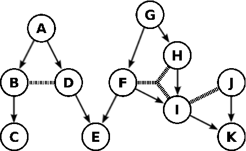
Figure 1 shows such a DAG for a set of tasks with arrows indicating the direction of the dependencies, i.e. an arrow from task $A$ to task $B$ indicates that task $B$ depends on task $A$ . In a parallel setting, tasks $A$ , $G$ , and $J$ can be executed concurrently. Once task $G$ has completed, tasks $F$ and $H$ become available and can be executed by any other computational thread.

Refer to caption — Figure 1: A set of tasks (circles) and their dependencies (arrows). The arrows indicate the direction of the dependency, i.e. an arrow from task $A$ to task $B$ indicates that task $B$ depends on task $A$ . Tasks $A$ , $G$ , and $J$ have no unsatisfied dependencies and can therefore be executed. Once task $G$ has completed, tasks $F$ and $H$ become available, and task $E$ only becomes available once both tasks $D$ and $F$ have completed.

One of the first implementations of a task-based parallel programming systems is Cilk (Blumofe et al.,, 1995), an extension to the C programming language which allows function calls to be “spawned” as new tasks. Dependencies are enforced by the sync keyword, which forces a thread to wait for all the tasks that it spawned to complete.

In SMP superscalar (Perez et al.,, 2008), StarPU (Augonnet et al.,, 2011), QUARK (YarKhan et al.,, 2011), and KAAPI (Gautier et al.,, 2007) the programmer specifies what shared data each task will access, and how that data will be accessed, e.g. read, write, or read-write access. The dependencies between tasks are then generated automatically by the runtime system, assuming that the data must be accessed and updated in the order in which the tasks are generated. StarPU also provides an interface for specifying additional dependencies explicitly. Intel’s Threading Building Blocks (TBB) (Reinders,, 2010) provide task-based parallelism using C++ templates in which dependencies are handled either by explicitly waiting for spawned tasks, or by explicitly manipulating task reference counters.

Finally, the very popular OpenMP standard provides some basic support for spawning tasks, similar to Cilk, as of version 3.0 (Board,, 2008). OmpSs (Duran et al.,, 2011) extends this scheme with automatic dependency generation as in SMP superscalar, of which it is a direct descendant, along with the ability to explicitly wait on certain tasks.

In all of these systems, the tasks are only aware of a single type of relationship between each other, i.e. dependencies, which specify a strict ordering between two tasks. In many cases, however, the task ordering need not necessarily be this strict. Consider the case of two tasks that update some shared resource in an order-independent way, e.g. when accumulating a result in a shared variable, or exclusively writing to an output file. In order to avoid concurrent access to that resource, it is imperative that the execution of both tasks does not overlap, yet the order in which the tasks are executed is irrelevant. In the following, such a relationship will be referred to as a conflict between two tasks. Figure 2 shows a task graph extended by conflicting tasks joined by thick dashed lines. None of tasks $F$ , $H$ , and $I$ can be executed concurrently, i.e. they must be serialized, yet in no particular order.

In dependency-only systems, such conflicts can be modelled with dependencies, which enforce a pre-determined arbitrary ordering on conflicting tasks. This artificial restriction on the order in which tasks can be scheduled can, however, severely limit the parallelizability of a computation, especially in the presence of multiple conflicts per task. Both Ltaief and Yokota, (2012) and Agullo et al., (2013) note this problem in their respective implementations of the Fast Multipole Method (FMM), in which forces computed in different tasks are accumulated on a set of particles.

Several libraries provide some mechanism to model such conflicts, either directly or indirectly. In the QUARK scheduler, conflicts can be modeled by explicitly marking dependencies as concurrent. KAAPI and OmpSS, on the other hand, allow marking access to certain variables as reductions, yet only for basic operations, e.g. summation or maximum/minimum.

This paper presents QuickSched, a framework for task-based parallel programming with constraints, which aims to achieve the following goals:

•

Correctness: All constraints, i.e. dependencies and conflicts, must be correctly enforced,
•

Speed: The overheads associated with task management should be as small as possible,
•

Memory/cache efficiency: Tasks accessing similar sets of data should be preferentially executed on the same core to preserve memory/cache locality as far as possible, and
•

Parallel efficiency: The order in which the tasks are executed should be chosen such that sufficient work is available for all computational threads at all times.

Section 2 describes the main design considerations, Section 3 the underlying algorithms and data structures, and Section 4 their specific implementation in QuickSched. Section 5 presents two test-cases:

1.

The tiled QR decomposition described in Buttari et al., (2009) and for which the QUARK scheduler was originally developed, and
2.

A task-based Barnes-Hut tree-code to compute the gravitational N-body problem similar to the FMM codes of Ltaief and Yokota, (2012) and Agullo et al., (2013),

These real-world examples show how QuickSched can be used in practice, and can be used to assess its efficiency. Section 6 concludes with some general observations and future work directions.

2 Design Considerations

From a programmer’s perspective, there are two main paradigms for generating task dependencies:

•

Implicitly via spawning and waiting, e.g. as is done in Cilk and OpenMP 3.0, or
•

Automatic extraction from data dependencies, e.g. as is done in StarPU, QUARK, and OmpSs.

The first scheme, spawning and waiting, is arguably the simplest to use. For simple depedency structures in which each task depends on only a single task, i.e. if the task DAG is a tree, each task spawns, or creates, its dependent tasks after its completion (see Figure 3a). Hence for the tasks $A$ – $E$ in Figure 1, task $A$ would spawn tasks $B$ and $D$ , task $B$ would spawn task $C$ , and task $D$ would spawn task $E$ . If a task has more than one dependency, e.g. tasks $D$ – $F$ in Figure 1, then the task generation order is reversed: Task $E$ is executed first, and first spawns tasks $D$ and $F$ , and waits for both their completion before doing its own computations (see Figure 3b).

Although simple to use, this implicit dependency management limits the types of DAGs that can be represented, e.g. for all the tasks in Figure 1, using such a spawning and waiting model would create implicit dependencies between the lowest-level tasks $C$ , $E$ , and $K$ . The main thread would spawn tasks $A$ , $G$ and $J$ , $A$ spawns $B$ and $D$ , $G$ spawns $F$ , $H$ , and then $I$ , $B$ spawns $C$ . The main thread then has to wait for $A$ , $G$ , and $J$ , and thus implicitly all their spawned tasks, before executing $E$ and $K$ .

Automatic dependency extraction, on the other hand, works by enforcing dependencies between tasks that access the same data. These data dependencies are provided explicitly by the programmer, e.g. by describing which parameters to a task are input, output, and input/output. The dependencies are enforced in the order in which the tasks are created. This approach usually relies on compiler extensions, e.g. pragmas in C/C++, or a system of function call wrappers, to describe the task parameters and their intent.

This approach allows programmers to specify rich dependency hierarchies with very little effort, i.e. without having to explicitly think about dependencies at all, yet they still only allow for one type of relationship, i.e. dependencies, and lack the ability to deal with conflicts as described in the previous section. They may also not be able to understand more complex memory access patterns, e.g. for two tasks modifying the upper and lower triangular parts of a matrix, which access the same block of memory, but never actually generate any concurrency issues.

Here, QuickSched takes a drastically different approach by requiring the programmer to create the complete task graph and its dependencies explicitly before execution. This approach has two main advantages:

•

It gives the user maximum flexibility with regards to the structure of the task graph generated,
•

Knowing the complete structure of the task graph before execution allows the task scheduler to make more informed decisions as to how the tasks should be prioritized.

The obvious disadvantage is the burden of producing a correct task graph is placed on the programmer. Although some problems such as cyclic dependencies can be detected automatically, there is no automatic way to detect whether the dependencies actualy reflect the intent of the programmer. Due to this added complexity, we consider QuickSched to be a tool not designed for casual parallel programmers, but for those interested in investing a bit more programming effort to achieve better performance.

As opposed to the dependencies, conflicts between tasks or groups of tasks are not specified directly, but are instead modeled as exclusive locks on a shared resource which have to be obtained by a task before it can execute. Thus, in Figure 2, before executing, task $F$ has to obtain an exclusive lock on the resource associated with the conflict between tasks $F$ , $H$ , and $I$ . While task $F$ is being executed, neither $H$ nor $I$ can lock the same resource, and therefore will not execute until task $F$ is done and the lock has been released.

As with all other task-based libraries, the partitioning of the computation into tasks is also left entirely to the programmer. In theory, any program can be automatically converted to a task-based representation since each statement in the program code can be considered a single task, with dependencies to the statements/tasks that produce the input values. This set of basic tasks could, again in theory, be reduced by merging tasks that share dependencies and/or resources using a variety of graph algorithms. The decomposition of a computation into tasks, however, usually involves re-thinking the underlying algorithms such that they best fit the task-based paradigm, e.g. as in the examples in the following sections, or as in Gonnet, (2014); Buttari et al., (2009); Ltaief and Yokota, (2012). This process requires careful evaluation of the underlying computation, and is probably best not left as an automatic transformation of an otherwise serial code.

Finally, the task granularity is an important issue: if the task decomposition is too coarse, then good parallelism and load-balancing will be difficult to achieve. Converseley, if the tasks are too small, the costs of selecting and scheduling tasks, which is usually constant per task, will quickly destroy any performance gains from parallelism. Starting from a per-statement set of tasks, it is therefore reasonable to group them by their dependencies and shared resources.

In the examples presented herein, we have chosen our task decomposition and granularity such that

•

Each task maximizes the ratio of computation to data required,
•

The resources required for each task fit comfortably in the lowest-level caches of the underlying system.

The first critera is biased towards bigger tasks, while the second limits their size. The parameters controlling the size of the tasks in the examples, i.e. the tile size in the QR decomposition and the limits $n_{\mathsf{max}}$ and $n_{\mathsf{task}}$ were determined empirically and only optimized to the closest power of two or rough power of ten, respectively. Further tuning these parameters could very likely lead to further performance gains, but such an effort would go beyond the scope, and point, of this paper.

3 Data Structures and Algorithms

The QuickSched task scheduler consists of four main objects types: task, resource, scheduler, and queue. The task and resource objects are used to model the computation, i.e. the work that is to be done and the data on which it will be done, respectively. The scheduler and queue objects manage how the work is done, i.e. which tasks get scheduled where and when, respectively.

The division of labor between the scheduler and the queue objects is illustrated in Figure 4. The scheduler holds the tasks and is in charge of managing dependencies. Once a task has no unresolved dependencies, it is passed on to a queue object. The queue object, on the other hand, is in charge of managing conflicts. Computational threads can query a queue and will receive only tasks for which all conflicts have been resolved, i.e. for which all necessary resources could be exclusively locked.

There is also a division of responsibilities regarding efficiency between the scheduler and the queue objects. The tasks in each queue are grouped according to the resources they use, i.e. all the tasks in the same queue use a similar set of resources. The underlying assumption is that each computational thread will preferentially access the same queue for tasks. If the tasks in the queue share the same set of resources, it increases the probability of said resources already being present in the thread’s cache, thus increasing cache efficiency. The scheduler is in charge of selecting the most appropriate queue for each task, based on information stored in each task on which resources are used. Given a set of tasks with similar resources for which all dependencies are resolved, it is up to the queue to decide which tasks to prioritize.

The following subsections describe these four object types in detail, as well as their operations.

3.1 Tasks

A task consists of the following data structure, in C-like pseudo-code:

⬇

1 struct task {

2 int type, wait;

3 void *data;

4 struct task **unlocks;

5 struct resource **locks, **uses;

6 int size_data, nr_unlocks, nr_locks, nr_uses;

7 int cost, weight;

8 };

where the data, unlocks, locks, and uses arrays are pointers to the contents of other arrays, i.e. they are not allocated individually.

What the task does is determined by the type field, e.g. which can be mapped to any particular function, and the data pointer which points to an array of size_data bytes containing data specific to the task, e.g. the parameters for a specific function call. Both fields are application-specific and therefore not important for the scheduler itself.

The unlocks field points to the first element of an array of nr_unlocks pointers to other tasks. These pointers represent the dependencies in reverse: if task $B$ depends on task $A$ , then task $A$ unlocks task $B$ . The unlocks therefore follow the direction of the arrows in Figures 1 and 2. Conversely, wait is the number of unresolved dependencies associated with this task, i.e. the number of unexecuted tasks that unlock this task. The wait-counters can be set by initializing all the task wait counters to zero and then incrementing the wait counter of each unlock-task of each task.

The locks field of each task points to the first element of an array of nr_locks pointers to resources for which exclusive locks must be obtained for the task to execute. Each locked resource represents a task conflict. Similarly, uses points to the first element of an array of nr_uses pointers to resources which will be used, but need not be locked.

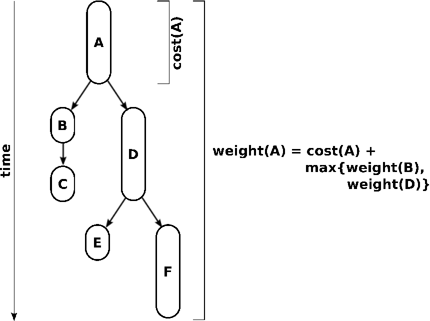
Finally, cost and weight are measures for the relative computational cost of this task, and the relative cost of the critical path following the dependencies of this task, respectively, i.e. the task’s cost plus the maximum dependent task’s weight (see Figure 5). The task cost can be either a rough estimate provided by the user, or the actual cost of the same task last time it was executed. The task weights are computed by traversing the tasks DAG in reverse topological order following their dependencies, e.g. as per Kahn, (1962) in $\mathcal{O}(n)$ for $n$ tasks, and computing each task’s weight, e.g.

\mbox{weight}_{i}=\mbox{cost}_{i}+\max_{j\in\mbox{\small unlocks}_{i}}\left\{\mbox{weight}_{j}\right\}.

where $\mbox{weight}_{i}$ and $\mbox{cost}_{i}$ are the weight and cost of the $i$ th task, respectively, and $\mbox{unlocks}_{i}$ is the set of tasks that the $i$ th task unlocks.

3.2 Resources

Resources consist of the following data structure:

⬇

1 struct resource {

2 struct resource *parent;

3 volatile int lock, hold;

4 int owner;

5 };

The parent field, which points to another resource, is used to create hierarchical resources, i.e. resources that are themselves subsets of larger resources. This can be useful, e.g. in the context of particle simulations described in the next section, where particles are sorted into hierarchical cells which are used at different levels. The owner field is the ID of the queue to which this resource has been preferentially assigned.

The lock field is either 0 or 1 and indicates whether this resource is currently in use, i.e. locked. To avoid race conditions, this value should be tested and set using atomic instructions only. The hold field is a counter indicating how many sub-resources of the current resource are locked. If a resource’s hold counter is not zero, then it is held and cannot be locked. Likewise, if a resource is locked, it cannot be held (see Figure 6).

Incrementing the hold counter of the resource can be implemented as follows:

⬇

1 void resource_hold(struct resource *r) {

2 if (atomic_cas(&r->lock, 0, 1) != 0) return 0;

3 atomic_inc(&r->hold);

4 r->lock = 0;

5 return 1;

6 }

where atomic_cas(val,old,new) is an atomic compare-and-swap operation that sets val to new if it is currently equal to old. Similarly, atomic_inc(val) increments val by one atomically. The resource’s lock is used to check if the resource is already locked (line 2), and it is held while hold is incremented, to avoid overlapping hold/lock operations. If the resource can be locked, the hold counter is incremented atomically (line 3), and the lock is released (line 4), returning 1 or 0 if the resource could be held or not, respectively.

The locking procedure itself is implemented as follows:

⬇

1 void resource_lock(struct resource *r) {

2 struct resource *up, *top;

3 if (r->hold && atomic_cas(&r->lock, 0, 1) != 0)

4 return 0;

5 if (r->hold) {

6 r->lock = 0;

7 return 0;

8 }

9 for (up = r->parent; up != NULL; up = up->parent)

10 if (!resource_hold(up)) break;

11 if ((top = up) != NULL) {

12 for (up = r->parent; up != top, up = up->parent)

13 atomic_dec(&up->hold);

14 r->lock = 0;

15 return 0;

16 } else

17 return 1;

18 }

where in line 3 the resource is first locked if it is not held. Due to a possible race condition when holding the resource, the hold counter must be checked again once the resource has been locked (line 5). In lines 9–10 the hold counters of the hierarchical parents are incremented using the procedure described earlier. If this process fails at any point (line 11), the previously set hold counters are decremented (line 13) and the lock is released (line 14). The procedure then returns 1 or 0 if the resource could be locked or not, respectively.

Finally, unlocking a resource is relatively straight-forward, i.e. the lock is set to zero and the hold counters up the resource hierarchy are decremented.

3.3 Queues

The main job of the task queues is, given a set of ready tasks, to find the task with maximum weight, i.e. the task along the longest critical path, whose resources can all be locked, and to do so as efficiently as possible.

One possible strategy would be to maintain an array of tasks sorted by their weights, and to traverse that list in descending order, trying to lock the resources of each task, until a lockable task is found, or returning a failure otherwise. Although this would return the best possible task, it requires maintaining a sorted array in which inserting or removing an entry is in ${\mathcal{O}}(n)$ for $n$ elements. Using an unsorted array would require only ${\mathcal{O}}(1)$ operations for insertion and deletion, but is undesirable as it completely ignores the task weights.

As a compromise, the queue stores the tasks in an array organized as a max-heap, i.e. where the $k$ th entry is “larger” than both the $2k+1$ st and the $2k+2$ nd entry, with the task with maximum weight in the first position. Maintaining this heap structure requires ${\mathcal{O}}(\log n)$ operations for both insertion and deletion, i.e. for the bubble-up and trickle-down operations respectively.

Unfortunately, there is no way of efficiently traversing all the elements in such a heap in decreasing order. The array of tasks is therefore traversed as if it were sorted, returning the first task that can be locked. Although the first task in the array will be the task with maximum weight, the following tasks are only loosely ordered, where the $k$ th of $n$ tasks has a larger weight than at least $\lfloor n/k\rfloor-1$ other tasks. Although this is not a particularly good lower bound, it turns out to be quite sufficient in practice.

The data structure for the queue is defined as follows:

⬇

1 struct queue {

2 struct task **tasks;

3 int count, lock;

4 };

where tasks is an array of count pointers to the tasks in max-heap order, and lock is used to guarantee exclusive access to the queue.

Inserting a task in the queue is relatively straight-forward:

⬇

1 void queue_put(struct queue *q, struct task *t) {

2 while (atomic_cas(q->lock, 0, 1) != 0) {}

3 q->tasks[q->count++] = t;

4 bubble-up the q->count - 1st entry of q->tasks.

5 q->lock = 0;

6 }

where the loop in line 2 spins until an exclusive lock on the queue can be obtained. The task is added to the end of the heap array (line 3) and the heap order is fixed (line 4). Before returning, the lock on the queue is released (line 5).

Obtaining a task from the queue can be implemented as follows:

⬇

1 struct task *queue_get(struct queue *q) {

2 struct task *res = NULL;

3 int j, k;

4 while (atomic_cas(q->lock, 0, 1) != 0) {}

5 for (k = 0; k < q->count; k++) {

6 for (j = 0; j < q->tasks[k]->nr_locks; j++)

7 if (!resource_lock(q->tasks[k]->lock[j])) break;

8 if (j < q->tasks[k]->nr_locks)

9 for (j = j - 1; j >= 0; j--)

10 resource_unlock(q->tasks[k]->lock[j]);

11 else

12 break;

13 }

14 if (k < q->count) {

15 res = q->tasks[k];

16 q->tasks[k] = q->tasks[--q->count];

17 trickle-down the kth entry of q->tasks.

18 }

19 q->lock = 0;

20 return res;

21 }

where, as with the queue insertion, the queue is first locked for exclusive access (line 4). The array of task pointers is then traversed (line 5), locking the resources of each task (lines 6–7). If any of these locks fail (line 8), the locks that were obtained are released (lines 9–10), otherwise, the traversal is aborted (line 12). If all the locks on a task could be obtained (line 14), the task pointer is replaced by the last pointer in the heap (line 16) and the heap order is restored (line 17). Finally, the queue lock is released (line 19) and the locked task, or NULL if no lockable task could be found, is returned.

Note that this approach of sequentially locking multiple resources is prone to the so-called “dining philosophers” problem, i.e. if two tasks attempt, simultaneously, to lock the resources $A$ and $B$ ; and $B$ and $A$ , respectively, via separate queues, their respective calls to queue_get will potentially fail perpetually. This type of deadlock, however, is easily avoided by sorting the resources in each task according to some global criteria, e.g. the resource ID or the address in memory of the resource.

Note also that protecting the entire queue with a mutex is not particularly scalable, and several authors, e.g. Sundell and Tsigas, (2003), have presented concurrent data structures that avoid this type of locking. However, since we normally use one queue per computational thread, contention will only happens due to work-stealing, i.e. when another idle computational thread tries to poach tasks. Since this happens only rarely, we opt for the simpler locking approach. This decision is backed by the results in Section 5.

3.4 Scheduler

The scheduler object is used as the main interface to the QuickSched task scheduler, and as such contains the instances of the other three object types:

⬇

1 struct qsched {

2 struct task *tasks;

3 struct queue *queues;

4 struct resource *res;

5 int nr_tasks, nr_queues, nr_resources;

6 volatile int waiting;

7 };

where the only additional field waiting is used to keep track of the number of tasks that have not been executed. Note that for brevity, and to avoid conflicts with the naming schemes of other standard libraries, the type name qsched is used for the scheduler data type.

The tasks are executed as follows:

⬇

1 void qsched_run(qsched *s, void (*fun)(int, void *)) {

2 qsched_start(s);

3 #pragma omp parallel

4 {

5 int qid = omp_get_thread_num() % s->nr_queues;

6 struct task *t;

7 while ((t = qsched_gettask(s, qid)) != NULL) {

8 fun(t->type, t->data);

9 qsched_done(s, t);

10 }

11 }

12 }

where qsched_start initializes the tasks and fills the queues (line 1). For simplicity, OpenMP (Dagum and Menon,, 1998), which is available for most compilers, is used to create a parallel section in which the code between lines 4 and 11 is executed concurrently. A version using pthreads (IEEE,, 1995) directly¹¹ 1 In most environments, OpenMP is implemented on top of pthreads, e.g. the gcc compiler’s libgomp. is also available. The parallel section consists of a loop (lines 7–10) in which a task is acquired via qsched_gettask and its type and data are passed to a user-supplied execution function fun. Once the task has been executed, it is returned to the scheduler via the function qsched_done, i.e. to unlock its resources and unlock dependent tasks. The loop terminates when the scheduler runs out of tasks, i.e. when qsched_gettask returns NULL, and the function exits once all the threads have exited their loops.

At the start of a parallel computation, qsched_start identifies the tasks that have no dependencies and sends them to queues via the function qsched_enqueue which tries to identify the best queue for a given task by looking at which queues last used the resources used and locked by the task, e.g.:

⬇

1 void qsched_enqueue(qsched *s, struct task *t) {

2 int best = 0, score[s->nr_queues];

3 for (int k = 0; k < s->nr_queues; k++)

4 score[k] = 0;

5 for (int k = 0; k < t->nr_locks; k++) {

6 int qid = t->locks[k]->owner;

7 if (++score[qid] > score[best]) best = qid;

8 }

9 for (int k = 0; k < t->nr_uses; k++) {

10 int qid = t->uses[k]->owner;

11 if (++score[qid] > score[best]) best = qid;

12 }

13 queue_put(&s->queues[best], t);

14 }

where the array score keeps a count of the task resources “owned”, or last used, by each queue. The task is then sent to the queue with the highest such score (line 13).

The function qsched_gettask fetches a task from one of the queues:

⬇

1 struct task *qsched_gettask(qsched *s, int qid) {

2 struct task *res = NULL;

3 int k;

4 while (s->waiting) {

5 if ((res = queue_get(s->queues[qid])) == NULL) {

6 loop over all other queues in random order with index k

7 if ((res = queue_get(s->queues[k])) != NULL)

8 break;

9 } else

10 break;

11 }

12 if (res != NULL && s->reown) {

13 for (k = 0; k < res->nr_locks; k++)

14 res->locks[k]->owner = qid;

15 for (k = 0; k < res->nr_uses; k++)

16 res->uses[k]->owner = qid;

17 }

18 return res;

19 }

where the parameter qid is the index of the preferred queue. If the queue is empty, or all of the tasks in that queue had unresolved conflicts, the scheduler uses a variant of the work stealing described in Blumofe and Leiserson, (1999), i.e. it loops over all other queues in a random order (line 6) and tries to get a task from them (line 7). If a task could be obtained from any queue and task re-owning is enabled (line 12), the resources it locks and uses are marked as now being owned by the preferred queue (lines 13–16). Finally, the task, or NULL if no task could be obtained, is returned.

The final step in a task’s life cycle is, on completion, to unlock the resources and tasks which depend on it. This is handled by the function qsched_done, which calls qsched_enqueue on any tasks for which the wait counter is decremented to zero. Once all the dependent tasks have been unlocked, the waiting counter of the scheduler is decremented.

4 Validation

This section presents two test cases that show how QuickSched can be used in real-world applications, and provides benchmarks to assess its efficiency and scalability. The first test is the tiled QR decomposition originally described in Buttari et al., (2009), which has been used as a benchmark by other authors (Agullo et al., 2009b, ; Badia et al.,, 2009; Bosilca et al.,, 2012). This example only requires dependencies and is presented as a point of comparison to existing task-based parallel programming infrastructures. The second example is a Barnes-Hut tree-code, a problem similar to the Fast Multipole Method described in both Ltaief and Yokota, (2012) and Agullo et al., (2013). This example shows how conflicts, modeled via hierarchical resources, can be useful in modelling and executing a problem efficiently.

The source code of both examples is distributed with the QuickSched library, along with scripts to run the benchmarks and generate the plots used in the following. All examples were compiled with gcc v. 5.2.0 using the -O2 -march=native flags and run on a 64-core AMD Opteron 6376 machine at 2.67 GHz.

4.1 Task-Based QR Decomposition

Buttari et al., (2009) introduced the concept of using task-based parallelism for tile-based algorithms in numerical linear algebra, presenting parallel codes for the Cholesky, LU, and QR decompositions. These algorithms are now part of the PLASMA and MAGMA libraries for parallel linear algebra (Agullo et al., 2009a, ). The former uses the QUARK task scheduler, which was originally designed for this specific task, while the latter currently uses the StarPU task scheduler (Agullo et al.,, 2011).

The tiled QR factorization is based on four basic tasks, or kernels, as shown in Figure 7. For a matrix consisting of $N\times N$ tiles, $N$ passes, or levels, are computed, each computing a column and row of the QR decomposition. The tasks can be defined in terms of the tuples $(i,j,k)$ , where $i$ and $j$ are the row and column of the tile, respectively, and $k$ is its level:

Task	where	depends on task(s)	locks tile(s)
DGEQRF	$i=j=k$	$(i,j,k-1)$	$(i,j)$
DLARFT	$i=k$ , $j>k$	$(i,j,k-1)$ , $(k,k,k)$	$(i,j)$
DTSQRF	$i>k$ , $j=k$	$(i,j,k-1)$ , $(i-1,j,k)$	$(i,j)$ , $(j,j)$
DSSRFT	$i>k$ , $j>k$	$(i,j,k-1)$ , $(i-1,j,k)$ , $(i,k,k)$	$(i,j)$

and where the task names are the BLAS-like operation performed on the given tiles. Every task depends on the task at the same position and the previous level, i.e. the task $(i,j,k)$ always depends on $(i,j,k-1)$ for $k>1$ . Each task also modifies its own tile $(i,j)$ , and the DTSQRF task additionally modifies the lower triangular part of the $(j,j)$ th tile.

Although the tile-based QR decomposition requires only dependencies, i.e. no additional conflicts are needed to avoid concurrent access to the matrix tiles, we still model each tile as a separate resource in QuickSched such that the scheduler can preferrentially assign tasks using the same tiles to the same thread. The resources/tiles are initially assigned to the queues in column-major order, i.e. the first $\lfloor n_{\mathsf{tiles}}/n_{\mathsf{queues}}\rfloor$ are assigned to the first queue, and so on.

The QR decomposition was computed for a $2048\times 2048$ random matrix using tiles of size $64\times 64$ floats using QuickSched as described above. The task costs were initialized to the asymptotic cost of the underlying operations. For this matrix, a total of 11 440 tasks with 21 824 dependencies, as well as 1 024 resources with 21 856 locks and 11 408 uses were generated.

For these tests, pthread parallelism and resource re-owning were used with one queue per core. The QR decomposition was computed 10 times for each number of cores, and the average thereof taken for the scaling and efficiency results in Figure 8. The timings are for qsched_run, including the cost of qsched_start, which does not run in parallel. Setting up the scheduler, tasks, and resources took, in all cases, an average of 7.2 ms, i.e. at most 3% of the total computational cost.

The same decomposition was implemented using OmpSs v. 1.99.0, calling the kernels directly using #pragma omp task annotations with the respective dependencies, and the runtime parameters

--disable-yield --schedule=socket --cores-per-socket=16
--num-sockets=4

Several different schedulers and parameterizations were discussed with the authors of OmpSs and tested, with the above settings producing the best results.

The scaling and efficiency relative to QuickSched are shown in Figure 8. The difference in timings is the result of the different task scheduling policies, as well as a smaller lag between the individual tasks, as shown in Figure 9, which shows the assignment of the different tasks to cores for the 64-core run. The most visible difference between both schedulers is that the DGEQRF tasks (in red) are scheduled as soon as they become available in QuickSched, thus preventing bottlenecks near the end of the computation.

Since in QuickSched the entire task structure is known explicitly in advance, the scheduler “knows” that the DGEQRF tasks all lie on the longest critical path and therefore executes them as soon as possible. OmpSs does not exploit this knowledge, resulting in the less efficient scheduling seen in Figure 9.

4.2 Task-Based Barnes-Hut N-Body Solver

The Barnes-Hut tree-code (Barnes and Hut,, 1986) is an algorithm to approximate the solution of an $N$ -body problem, i.e. computing all the pairwise interactions between a set of $N$ particles, in ${\mathcal{O}}(N\log N)$ operations, as opposed to in ${\mathcal{O}}(N^{2})$ for the naive direct computation. The algorithm is based on a recursive octree decomposition: Starting from a cubic cell containing all the particles, the cell is recursively bisected along all three spatial dimensions, resulting in eight sub-cells, until the number of particles per cell is smaller than some limit $n_{\mathsf{max}}$ . The particle interactions can then be formulated recursively: Given a particle and a set of particles in a cell, if the particle and cell are sufficiently well separated, the particle-cell interactions are approximated by interacting the particle with the cell’s center of mass. If the particle and the cell are too close, and the cell has sub-cells, i.e. it contained more than $n_{\mathsf{max}}$ particles and was split in the recursive octree decomposition, then the particle is interacted with each of the sub-cells recursively. Finally, if the cell is not split, i.e. it is a leaf cell in the octree, then the particle is interacted with all particles in the cell, except for the particle itself if it is in the same cell. This operation is performed for each particle, starting with the root-level cell containing all the particles.

In our implementation, the particle data is sorted hierarchically, following the octree structure. Unlike in many codes, where the leaves store an array of pointers to the underlying particles, which are not necessarily contiguous in memory, the cells, at all levels, store only a pointer to the first of their own particles, and the total number of particles. The current approach, illustrated in Figure 10 is not only more compact, it also allows a direct and more cache-efficient access to the list of particles for any inner node of the tree. The cost of sorting the particles, with a recursive partitioning similar to QuickSort (Hoare,, 1962), is in ${\mathcal{O}}(N\log N)$ .

The task-based implementation consists of three types of tasks:

•

Self-interactions, in which all particles in a single cell interact with all other particles in the same cell,
•

Particle-particle pair interactions, in which all particles in a cell interact with all particles in another cell,
•

Particle-cell pair interactions, in which all particles in one cell are interacted with the center of mass of all other cells in the tree.

These tasks can be created recursively over the cell hierarchy as shown in the function make_tasks in Figure 16. The function is called on the root cell with the root cell and NULL as its two cell parameters. The function recurses as follows (line numbers refer to Figure 16:

•

If called with a single, split cell (lines 6–7), recurse over all the cell’s sub-cells, and all pairs of the cell’s sub-cells (lines 8–11),
•

If called with a single unsplit cell (line 13), create a self-interaction task (line 14) as well as a particle-cell task on that cell (line 18),
•

If called with two neighbouring cells and both cells are split (line 22), recurse over all pairs of sub-cells spanning both cells (lines 24–26), and
•

If called with two neighbouring cells and at least one of the cells is not split, create a particle-particle pair task over both cells (line 29),
•

If called with two non-neighbouring cells, do nothing, as these interactions will be computed by the particle-cell task.

Every interaction task additionally locks the cells on which it operates (lines 17, 20, and 32–33). In order to prevent generating a large number of very small tasks, the task generation only recurses if the cells contain more than a minimum number $n_{\mathsf{task}}$ of particles each (lines 7 and 23).

As shown in Figure 15, the particle-self and particle-particle pair interaction tasks are implemented by computing the interactions between all particle pairs spanning both cells in a double for-loop (lines 9–11 and 22-24 therein). Some extra logic (lines 2–7 and 15–20) is added to deal with split cells that did not contain enough particles to warrant the generation of finer tasks. The particle-cell interactions for each leaf node are computed by traversing the tree recursively starting from the root node and:

•

If called with a node that is a hierarchical parent of the leaf node, or with a node that is a direct neighbour of a hierarchical parent of the leaf node, recurse over the node’s sub-cells (lines 29–32),
•

Otherwise, compute the interaction between the leaf node’s center of mass and all the particles in the leaf node (lines 33–35).

This task decomposition differs from the traditional tree-walk in the Barnes-Hut algorithm in that the particle-cell interactions are grouped per leaf, with each leaf doing its own tree walk, as opposed to doing a tree walk for each individual particle. This approach was chosen to maximize the memory locality of the particle-cell calculation, as the particles in the leaf, which are traversed for each particle-cell interaction, are contiguous in memory, and are thus more likely to remain in the lowest-level cache during the entire tree-walk.

This Barnes-Hut tree-code was used to approximate the gravitational N-Body problem for 1 000 000 particles with uniformly random coordinates in $[0,1]^{3}$ . The parameters $n_{\mathsf{max}}=100$ and $n_{\mathsf{task}}=5000$ were used to generate the tasks. Using the above scheme generated 97 553 tasks, of which 512 self-interaction tasks, 5 068 particle-particle interaction task, and 32 768 particle-cell interaction tasks. A total of 43 416 locks on 37 449 resources were generated. Setting up the tasks took, on average XXX ms, i.e. at most XXX% of the total computation time. Storing the tasks, resources, and dependencies required XXX MB, which is only XX% of the XXX MB required to store the particle data.

For these tests, pthreads parallelism was used and resource re-owning was switched off. Resource ownership was attributed by dividing the global parts array by the number of queues and assigning each cell’s res to the fraction of the parts array to which the first of its own parts belong. The interactions were computed 10 times for each number of cores, and the average thereof taken for the scaling and efficiency results in Figure 11. The timings are for qsched_run, including the cost of qsched_start, which does not run in parallel. Setting up the scheduler, tasks, and resources took, in all cases, an average of 51.3 ms.

For comparison, the same computations were run using the popular astrophysics simulation software Gadget-2 (Springel,, 2005), using a traditional Barnes-Hut implementation based on octrees and distributed-memory parallelism based on domain decompositions and MPI (Snir et al.,, 1998). To achieve the same accuracy, an opening angle of 0.5 was used. On a single core, the task-based tree traversal is already 1.9 $\times$ faster than Gadget-2, due to the cache efficiency of the task-based computations, which, by design, maximize the amount of computation per memory access. At 59 cores, where Gadget-2 performs best, the task-based tree traversal is 2.51 $\times$ faster, and at the full 64 cores it is 4 $\times$ faster, due to the better strong scaling of the task-based approach as opposed to the MPI-based parallelism in Gadget-2.

Unlike the QR decomposition, the results scale well only to 32 cores, achieving 90% parallel efficiency, and then level off for increasing numbers of cores. This, however, is not a problem of the task-based parallel algorithm, or of QuickSched, but of the memory bandwidth of the underlying hardware. Figure 13 shows the accumulated cost of each task type and of QuickSched over the number of cores. At 64 cores, the scheduler overheads account for only $\sim 1$ % of the total computational cost, whereas, as of 32 cores, the cost of both pair types grow by up to 40%. This is due to the cache hierarchy of the AMD Opteron 6376 in which pairs of cores share a comon 2 MB L2 cache. When using half the cores or less, each core has its L@ cache to itself, whereas beyond 32 cores they are shared, resulting in more frequent cache misses. This cen be seen when comparing the costs of the particle-particle interaction and particle-cell interaction tasks: while the former grow by roughly 30%, the latter grow by only 10% as they do much more computation per memory access.

5 Discussion and Conclusions

The task scheduler described in the previous sections, QuickSched, differs from existing task-based programming schemes in a number of ways. The most obvious such difference is the addition of conflicts, modeled using exclusive locks on hierarchical resources. This extension to the standard dependencies-only model of task-based parallelism allows for more complex task relations, such as in the Barnes-Hut tree-code described earlier.

Another significant difference is that the tasks, their dependencies, and their conflicts must be described explicitly before the parallel computation starts. This as opposed to implicit dependencies generated by task spawning, e.g. as in Cilk, or to extracting the dependencies from the task parameters, e.g. in QUARK or OmpSs. Explicitly defining dependencies has the advantage that more elaborate dependency structures can be generated. Furthermore, knowing the structure of the entire task graph from the start of the computation provides valuable information when scheduling the tasks, e.g. using the critical path along the dependencies to compute the task weight.

Finally, as opposed to the most other task-based programming environments which rely on compiler extensions and/or code pre-processors, QuickSched operates as a regular C-language library, based on standard parallel functionality provided by OpenMP and/or pthreads. This ensures a maximum amount of portability on existing and future architectures. The interfaces are also kept as simple as possible in order to reduce the burden on the programmer when implementing task-based codes.

The QuickSched library itself is remarkably simple, consisting of less than 3 000 lines of code, including comments. Both examples, which are distributed with QuickSched, require less than 1 000 lines of code each. For a more complex, large-scale example of a task-based computation based on the same algorithms, we refer to Gonnet, (2014), for which the scheduler was originally designed, and from which QuickSched was back-ported.

In both examples, QuickSched performs extremely well, even on a large number of shared-memory cores. This performance is due, on the one hand, to the division of labor between the scheduler and the queues, and on the other hand due to the simple yet efficient algorithms for task selection and resource locking. The task weighting based on the length of the critical path of the dependencies delivers, in the examples shown, good parallel efficiency.

There are several possible improvements to QuickSched which have not been addressed in this paper. The most obvious of which are the following:

•

Priorities: The current implementation of QuickSched does not take the resource locks into account when selecting tasks in the queues, e.g. it may be advantageous, in some settings, to avoid tasks which are involved in too many potential conflicts and would therefore restrict the maximum degree of parallelism when scheduled.
•

Work-stealing: During work-stealing, the queues are probed in a random order although the total relative cost of the tasks in the queue, as well as the length of their critical paths are known,
•

Costs: The size of the resources used by a task are currently not taken into account when assigning it to the queues in qsched_enqueue, or when approximating the cost of a task.

QuickSched is distributed under the GNU Lesser General Public Licence v 3.0 and is available for download via https://sourceforge.net/projects/quicksched/files/.

Acknowledgments

The authors would like to thank Tom Theuns and Richard Bowers of the Institute for Computational Cosmology at Durham University for the helpful discussions. This work was supported by a Durham University Seedcorn Grant number 21.12.080130 from which the hardware used in the experiments was purchased.

References

Agullo et al., (2011) Agullo, E., Augonnet, C., Dongarra, J., Faverge, M., Ltaief, H., Thibault, S., and Tomov, S. (2011). QR Factorization on a Multicore Node Enhanced with Multiple GPU Accelerators. In 25th IEEE International Parallel & Distributed Processing Symposium, Anchorage, États-Unis.
Agullo et al., (2013) Agullo, E., Bramas, B., Coulaud, O., Darve, E., Messner, M., and Takahashi, T. (2013). Task-based FMM for multicore architectures. Technical Report 8277, Inria, Domaine de Voluceau – Rocquencourt, BP 105–78153, Le Chesnay, Cedex.
(3) Agullo, E., Demmel, J., Dongarra, J., Hadri, B., Kurzak, J., Langou, J., Ltaief, H., Luszczek, P., and Tomov, S. (2009a). Numerical linear algebra on emerging architectures: The PLASMA and MAGMA projects. In Journal of Physics: Conference Series, volume 180, page 012037. IOP Publishing.
(4) Agullo, E., Hadri, B., Ltaief, H., and Dongarrra, J. (2009b). Comparative study of one-sided factorizations with multiple software packages on multi-core hardware. In Proceedings of the Conference on High Performance Computing Networking, Storage and Analysis, page 20. ACM.
Augonnet et al., (2011) Augonnet, C., Thibault, S., Namyst, R., and Wacrenier, P.-A. (2011). StarPU: A unified platform for task scheduling on heterogeneous multicore architectures. Concurrency and Computation: Practice and Experience, Special Issue: Euro-Par 2009, 23:187–198.
Badia et al., (2009) Badia, R. M., Herrero, J. R., Labarta, J., Pérez, J. M., Quintana-Ortí, E. S., and Quintana-Ortí, G. (2009). Parallelizing dense and banded linear algebra libraries using SMPSs. Concurrency and Computation: Practice and Experience, 21(18):2438–2456.
Barnes and Hut, (1986) Barnes, J. and Hut, P. (1986). A hierarchical o (n log n) force-calculation algorithm. Nature.
Blumofe et al., (1995) Blumofe, R. D., Joerg, C. F., Kuszmaul, B. C., Leiserson, C. E., Randall, K. H., and Zhou, Y. (1995). Cilk: an efficient multithreaded runtime system. In Proceedings of the fifth ACM SIGPLAN symposium on Principles and practice of parallel programming, PPOPP ’95, pages 207–216, New York, NY, USA. ACM.
Blumofe and Leiserson, (1999) Blumofe, R. D. and Leiserson, C. E. (1999). Scheduling multithreaded computations by work stealing. Journal of the ACM (JACM), 46(5):720–748.
Board, (2008) Board, O. (2008). Openmp application program interface version 3.0. In The OpenMP Forum, Tech. Rep.
Bosilca et al., (2012) Bosilca, G., Bouteiller, A., Danalis, A., Herault, T., Lemarinier, P., and Dongarra, J. (2012). DAGuE: A generic distributed dag engine for high performance computing. Parallel Computing, 38(1):37–51.
Buttari et al., (2009) Buttari, A., Langou, J., Kurzak, J., and Dongarra, J. (2009). A class of parallel tiled linear algebra algorithms for multicore architectures. Parallel Computing, 35(1):38–53.
Dagum and Menon, (1998) Dagum, L. and Menon, R. (1998). OpenMP: an industry standard API for shared-memory programming. Computational Science & Engineering, IEEE, 5(1):46–55.
Duran et al., (2011) Duran, A., Ayguadé, E., Badia, R. M., Labarta, J., Martinell, L., Martorell, X., and Planas, J. (2011). OmpSs: a proposal for programming heterogeneous multi-core architectures. Parallel Processing Letters, 21(02):173–193.
Gautier et al., (2007) Gautier, T., Besseron, X., and Pigeon, L. (2007). Kaapi: A thread scheduling runtime system for data flow computations on cluster of multi-processors. In Proceedings of the 2007 international workshop on Parallel symbolic computation, pages 15–23. ACM.
Gonnet, (2014) Gonnet, P. (2014). Efficient and scalable algorithms for smoothed particle hydrodynamics on hybrid shared/distributed-memory architectures. SIAM Journal on Scientific Computing, in Press.
Hoare, (1962) Hoare, C. A. (1962). Quicksort. The Computer Journal, 5(1):10–16.
IEEE, (1995) IEEE (1995). Posix.1c, threads extension. IEEE Std 1003.1.
Kahn, (1962) Kahn, A. B. (1962). Topological sorting of large networks. Communications of the ACM, 5(11):558–562.
Ltaief and Yokota, (2012) Ltaief, H. and Yokota, R. (2012). Data-driven execution of fast multipole methods.
Perez et al., (2008) Perez, J. M., Badia, R. M., and Labarta, J. (2008). A dependency-aware task-based programming environment for multi-core architectures. In Cluster Computing, 2008 IEEE International Conference on, pages 142–151. IEEE.
Reinders, (2010) Reinders, J. (2010). Intel threading building blocks: outfitting C++ for multi-core processor parallelism. O’Reilly Media, Inc.
Snir et al., (1998) Snir, M., Otto, S., Huss-Lederman, S., Walker, D., and Dongarra, J. (1998). MPI: The Complete Reference (Vol. 1): Volume 1-The MPI Core, volume 1. MIT press.
Springel, (2005) Springel, V. (2005). The cosmological simulation code gadget-2. Monthly Notices of the Royal Astronomical Society, 364(4):1105–1134.
Sundell and Tsigas, (2003) Sundell, H. and Tsigas, P. (2003). Fast and lock-free concurrent priority queues for multi-thread systems. In Parallel and Distributed Processing Symposium, 2003. Proceedings. International, pages 11–pp. IEEE.
YarKhan et al., (2011) YarKhan, A., Kurzak, J., and Dongarra, J. (2011). Quark users’ guide: Queueing and runtime for kernels. Technical Report ICL-UT-11-02, University of Tennessee Innovative Computing Laboratory.

Appendix A User Interface

This section describes the QuickSched interface functions and how they are called.

As mentioned previously, the qsched object is the main interface to the task scheduler. As such, it provides functionality for task and resource creation, for assigning resources to tasks, either as locks or uses, and for assigning dependencies between tasks. The tasks and resources themselves are opaque to the user, and handles of the types qsched_task_t and qsched_res_t are used instead.

The main functions for setting up the scheduler are:

•

void qsched_init(struct qsched *s, int nr_queues, int flags)
Initializes a qsched object with the given number of queues. The flags parameter can be set to any bitwise or combination of qsched_flag_none, qsched_flag_yield, and qsched_flag_pthread, which are described further below. This function must be called before any of the other functions are used.
•

void qsched_free(struct qsched *s)
Releases all the memory and other resources allocated by the given qsched object. After this function has been called, the qsched will need to be re-initialized for reuse.
•

void qsched_reset(struct qsched *s)
Clears the tasks and resources in the given qsched, but does not release the allocated memory or change the number of queues.
•

qsched_task_t qsched_addtask(struct qsched *s, int type, unsigned int flags, void *data, int data_size, int cost)
Creates a new task within the given qsched and returns its handle. The type and data field are copied into the qsched and passed to the execution function when the qsched is run. The parameter flags is either task_flag_none or task_flag_virtual. Tasks marked as virtual do not have any action associated with them, e.g. they are used only to group or otherwise dependencies, and are not passed to the execution function in qsched_run.
•

qsched_res_t qsched_addres(struct qsched *s, int owner, qsched_res_t parent)
Creates a new resource within the given qsched and returns its handle. The owner field is the initial queue ID to which this resource should be assigned, or qsched_owner_none. The parent field is the handle of the hierarchical parent of the new resource or qsched_res_none if the resource has no hierarchical parent.
•

void qsched_addlock(struct qsched *s, qsched_task_t t, qsched_res_t res)
Append the resource res to the task t’s list of locks. The task t will then conflict with any other task that also locks the resource res, its hierarchical parents, or any resource hierarchically below it.
•

void qsched_adduse(struct qsched *s, qsched_task_t t, qsched_res_t res)
Similar to qsched_addlock, yet the resource is only used and is not part of a conflict. This information is used when assigning tasks to specific queues.
•

void qsched_addunlock(struct qsched *s, qsched_task_t ta, qsched_task_t tb)
Appends the task tb to the list of tasks that the task ta unlocks. The task tb then depends on the task ta.
•

void qsched_run(struct qsched *s, int nr_threads, qsched_funtype fun)
Executes the tasks in the given qsched using nr_threads threads via the execution function fun, as described in the previous section. Once a qsched has been initialized and filled with tasks and resources, it can be run more than once.

The library can be compiled to use OpenMP and/or the pthreads library. OpenMP is the default, but calling qsched_init with either the qsched_flag_yield or the qsched_flag_pthread switches to using pthreads, if available, for the parallel loop.

OpenMP has the advantage of being available for most compilers and also potentially providing some extra platform-specific scheduling features, e.g. optimal thread location and/or affinity, and of integrating seamlessly with other parallel parts of the user application. The disadvantage of using OpenMP is that it does not provide any mechanism for yielding a thread if no tasks are available, i.e. the main loop in qsched_gettask, described in the previous section, will spin until a task becomes available. This may be a problem if other parts of the user application are running concurrently in the background outside of QuickSched. Calling qsched_init with the qsched_flag_yield forces the use of pthreads and uses conditional variables to wait for a new task to be enqueued if obtaining a task from any of the queues fails. This relinquishes the waiting computational thread for other processes.

Appendix B Tiled QR Implementation

⬇

1 enum {tDGEQRF, tDLARFT, tDTSQRF, tDSSRFT};

2 void make_tasks(struct qsched *s, int m, int n) {

3 int i, j, k, data[3];

4 qsched_task_t tid[m * n], tid_new;

5 qsched_res_t rid[m * n];

6 for (k = 0; k < m * n; k++) {

7 tid[k] = qsched_task_none;

8 rid[k] = qsched_addres(s, qsched_res_none);

9 }

10 for (k = 0; k < m && k < n; k++) {

11 /* DGEQRF task at (k,k). */

12 data[0] = k; data[1] = k; data[2] = k;

13 tid_new = qsched_addtask(s, tDGEQRF, qsched_flags_none, data,

14 sizeof(int) * 3, 2);

15 qsched_addlock(s, tid_new, rid[k * m + k])

16 if (tid[k * m + k] != qsched_task_none)

17 qsched_addunlock(s, tid[k * m + k], tid_new);

18 tid[k * m + k] = tid_new;

19 for (j = k + 1; j < n; j++) {

20 /* DLARFT task at (k,j). */

21 data[0] = k; data[1] = j; data[2] = k;

22 tid_new = qsched_addtask(s, tDLARFT, qsched_flags_none, data,

23 sizeof(int) * 3, 3);

24 qsched_addlock(s, tid_new, rid[j * m + k])

25 qsched_addunlock(s, tid[k * m + k], tid_new);

26 if (tid[j * m + k] != qsched_task_none)

27 qsched_addunlock(s, tid[j * m + k], tid_new);

28 tid[j * m + k] = tid_new;

29 }

30 for (i = k + 1; i < m; i++) {

31 /* DTSQRF task at (i,k). */

32 data[0] = i; data[1] = k; data[2] = k;

33 tid_new = qsched_addtask(s, tDTSQRF, qsched_flags_none, data,

34 sizeof(int) * 3, 3);

35 qsched_addlock(s, tid_new, rid[k * m + i])

36 qsched_addlock(s, tid_new, rid[k * m + k])

37 qsched_addunlock(s, tid[k * m + k], tid_new);

38 if (tid[k * m + i] != qsched_task_none)

39 qsched_addunlock(s, tid[k * m + i], tid_new);

40 tid[k * m + i] = tid_new;

41 for (j = k + 1; j < n; j++) {

42 /* DSSRFT task at (i,j). */

43 data[0] = i; data[1] = j; data[2] = k;

44 tid_new = qsched_addtask(s, tDSSRFT, qsched_flags_none, data,

45 sizeof(int) * 3, 5);

46 qsched_addlock(s, tid_new, rid[j * m + i])

47 qsched_addunlock(s, tid[j * m + k], tid_new);

48 qsched_addunlock(s, tid[k * m + i], tid_new);

49 if (tid[j * m + i] != qsched_task_none)

50 qsched_addunlock(s, tid[j * m + i], tid_new);

51 tid[j * m + i] = tid_new;

52 }

53 }

54 }

55 }

Figure 14: Example code to generate the tasks for the tiled QR decomposition.

Setting up the dependencies and locks for a matrix of $m\times n$ tiles is implemented as shown in Figure 14, where the $m\times n$ matrix tid stores the handles of the last task at position $(i,j)$ and is initialized with empty tasks (line 7). Similarly, rid stores the handles of the resources for each tile of the matrix, which are allocated in line 8.

The following loops mirror the task generation described in Algorithm 2 of (Buttari et al.,, 2009). For each level k (line 10), a DGEQRF task is created for tile $(k,k)$ (lines 13–14). A lock is added for the newly created task on the resource associated with the $(k,k)$ th tile (line 15). If a task exists at that position at the previous level (line 16), a dependency is added between the old task and the new (line 17), and the new task is stored in tid (line 18). The remaining tasks are generated in the same way, with their respective locks and dependencies.

The execution function for these tasks simply calls the appropriate kernels on the matrix tiles given by the task data:

⬇

1 void exec_fun(int type, void *data) {

2 int *idata = (int *)data;

3 int i = idata[0], j = idata[1], k = idata[2];

4 switch (type) {

5 case tDGEQRF:

6 DGEQRF(A[i, j], ...);

7 break;

8 case tDLARFT:

9 DLARFT(A[i, j], A[i, i], ...);

10 break;

11 case tDTSQRF:

12 DTSQRF(A[i, j], A[j, j], ...);

13 break;

14 case tDSSRFT:

15 DSSRFT(A[i, j], A[i, k], A[k, j], ...);

16 break;

17 default:

18 error("Unknown␣task␣type.");

19 }

20 }

where A is the matrix over which the QR decomposition is executed.

Appendix C Barnes-Hut N-body Solver Implementation

The cells themselves are implemented using the following data structure:

⬇

1 struct cell {

2 double loc[3], h[3], com[3], mass;

3 int split, count;

4 struct part *parts;

5 struct cell *progeny[8];

6 qsched_res_t res;

7 qsched_task_t task_com;

8 };

where loc and h are the location and size of the cell, respectively. The com and mass fields represent the cell’s center of mass, which will be used in the particle-cell interactions. The res filed is the hierarchical resource representing the cell’s particles, and it is the parent resource of the cell progeny’s res. Similarly, the task_com is a task handle to compute the center of mass of the cell’s particles, and it depends on the task_com of all the progeny if the cell is split. parts is a pointer to an array of count particle structures, which contain all the particle data of the form:

⬇

1 struct part {

2 double x[3], a[3], mass;

3 int id;

4 };

i.e. the particle position, acceleration, mass, and ID, respectively.

⬇

1 void comp_self(struct cell *c) {

2 if (c->split) {

3 for (int j = 0; j < 8; j++) {

4 comp_self(c->progeny[j]);

5 for (int k = j + 1; k < 8; k++)

6 comp_pair(c->progeny[j], c->progeny[k]);

7 }

8 } else {

9 for (int j = 0; j < c->count; j++)

10 for (int k = j + 1; k < c->count; k++)

11 interact c->parts[j] and c->parts[k].

12 }

13 }

15 void comp_pair(struct cell *ci, struct cell *cj) {

16 if (ci and cj are not neighbours)

17 return;

18 if (ci->split && cj->split) {

19 for (int j = 0; j < 8; j++)

20 for (int k = 0; k < 8; k++)

21 comp_pair(ci->progeny[j], cj->progeny[k]);

22 } else {

23 for (int j = 0; j < ci->count; j++)

24 for (int k = 0; k < cj->count; k++)

25 interact ci->parts[j] and cj->parts[k].

26 }

27 }

29 void comp_pair_cp(struct cell *leaf, struct cell *c) {

30 if (c is a parent of leaf ||

31 c is a neighbour of a parent of leaf) {

32 for (int k = 0; k < 8; k++)

33 comp_pair_cp(leaf, c->progeny[k]);

34 } else if (leaf and c are not direct neighbours) {

35 for (int k = 0; k < leaf->count; k++)

36 interact leaf->parts[k] and c center of mass.

37 }

38 }

Figure 15: Task functions for the Barnes-Hut tree-code.

⬇

1 enum { tSELF, tPAIR_PP, tPAIR_PC };

2 void make_tasks(struct qsched *s, struct cell *ci, struct cell *cj) {

3 int j, k;

4 qsched_task_t tid;

5 struct cell *data[2];

6 if (cj == NULL) {

7 if (ci->split && ci->count > n_task) {

8 for (j = 0; j < 8; j++) {

9 make_tasks(s, ci->progeny[j], NULL);

10 for (k = j + 1; k < 8; k++)

11 make_tasks(s, ci->progeny[j], ci->progeny[k]);

12 }

13 } else {

14 tid = qsched_addtask(s, tSELF, qsched_flags_none, &ci,

15 sizeof(struct cell *),

16 ci->count * ci->count);

17 qsched_addlock(s, tid, ci->res);

18 tid = qsched_addtask(s, tPAIR_PC, qsched_flags_none, &ci,

19 sizeof(struct cell *), ci->count);

20 qsched_addlock(s, tid, ci->res);

21 }

22 } else if (ci->split && cj->split &&

23 ci->count * cj->count > n_task * n_task) {

24 for (j = 0; j < 8; j++)

25 for (k = 0; k < 8; k++)

26 make_tasks(s, ci->progeny[j], cj->progeny[k]);

27 } else {

28 data[0] = ci; data[1] = cj;

29 tid = qsched_addtask(s, tPAIR_PP, qsched_flags_none, data,

30 sizeof(struct cell *) * 2,

31 ci->count * cj->count);

32 qsched_addlock(s, tid, ci->res);

33 qsched_addlock(s, tid, cj->res);

34 }

35 }

Figure 16: C-like pseudo-code for recursive task creation for the Barnes-Hut tree-code.

The functions for the task themselves are relatively straight-forward and shown in Figure 15, and the execution function can be written as:

⬇

1 void exec_fun(int type, void *data) {

2 struct cell **cells = (struct cell **)data;

3 switch (type) {

4 case tSELF:

5 comp_self(cells[0]);

6 break;

7 case tPAIR_PP:

8 comp_pair(cells[0], cells[1]);

9 break;

10 case tPAIR_PC:

11 comp_pair_pc(cells[0], root);

12 break;

13 case tCOM:

14 comp_com(cells[0]);

15 break;

16 default:

17 error("Unknown␣task␣type.");

18 }

19 }