Towards Programmable Network Dynamics:
A Chemistry-Inspired Abstraction for Hardware Design
Abstract
Chemical algorithms are statistical algorithms described and represented as chemical reaction networks. They are particularly attractive for traffic shaping and general control of network dynamics; they are analytically tractable, they reinforce a strict state-to-dynamics relationship, they have configurable stability properties, and they are directly implemented in state-space using a high-level (graphical) representation. In this paper, we present a direct implementation of chemical algorithms on FPGA hardware. Besides substantially improving performance, we have achieved hardware-level programmability and re-configurability of these algorithms at runtime (not interrupting servicing) and in realtime (with sub-second latency). This opens an interesting perspective for expanding the currently limited scope of software defined networking and network virtualisation solutions, to include programmable control of network dynamics.
Index Terms:
Chemical algorithm, Programmable networks, Software defined networking, Network dynamics, Traffic shaping, FPGA.I Introduction
Network dynamics as a term describes an important operational aspect of queuing networks and the Internet. It refers to traffic control processes such as (among others) scheduling, shaping, policing, and Active Queue Management (AQM). Initially, network dynamics were controlled end-to-end only, through transport protocol mechanisms such as TCP’s flow and congestion control algorithms. Yet today, also mechanisms at the core of the network play an important role in shaping intra/inter-flow dynamics in the Internet. This is effected for example by means of service differentiation, flow conditioning, (distributed) rate control, AQM and other congestion avoidance measures.
Recent developments in network virtualisation for cloud infrastructures and Software Defined Networking (SDN), which explore ways to make network infrastructure runtime-volatile through software, have at large neglected network dynamics. To date, most of efforts have focused on programmability of data paths (functions pertinent to firewalling, packet inspection, header editing, etc.) and topology management. In regard to network dynamics on the other hand, while notable advancements are being underway today [1]–[8], programmable SDN-like deployments are at best confined to a number of pre-packaged (often “age-old”) algorithms, typically offered as proprietary manufacturer-provided modules [9]. A potentially notable exception is the software-switch specification language proposed in [10]. Authors claim that it may be used to create action primitives for congestion control although they fall short of explaining how (or providing examples).
Enabling runtime programmability/configurability of functions to control network dynamics is more challenging than accessing and modifying the router/node fabric to simply extend packet parsing and filtering functionalities (e.g., [11, 12]) or perform topology management (e.g., [13]). First of all, it requires solutions that can be deployed close to, or on, hardware (for performance and computational speed reasons). Additionally, in contrast to a mere flow-rule pipeline, such functions are algorithmically complex to implement, with many interdependencies to cater for. For example, programming or reconfiguring a queueing discipline often requires to modify the actual logic [6, 7, 14] that functionally binds different runtime parameters and components (e.g. queue-lengths, filter thresholds, droppers and markers, averaging coefficients, etc.). Next, management operations for modifying parameters in these functions (e.g. setting rate cap parameters, meter bands, etc.) are likely more frequent than typical topology management tasks. And finally, changes (not only modifications but also the replacement of algorithms) are less tolerant to data-path delays than load operations of flow-table rules.
In past works [15]–[20], we have introduced a class of algorithms founded on operational principles of chemical reaction networks, and demonstrated their suitability for (expressible state-space representation) and usefulness in (analysability/verification) the design of control functions for various tasks pertinent to network dynamics. In this paper, we capitalise on, and complete, this work in the context of programmable networks, and we show that these “chemical” algorithms (CAs) are fast to deploy and easy to re-program and modify at runtime on FPGA hardware. Specifically the contributions of this work amount to the following:
- 1.
Direct expressibility of high level mathematical models of control systems on hardware, based on the simple reaction network abstraction, without resorting to cumbersome hardware description language (HDL) programming.
- 2.
Effective algorithmic parallelisation without special engineering effort or the need for compiler optimisation. As these models freely describe parallelisable logic in state equations, they do not need to be implemented as finite state automata (i.e. sequentialised algorithms) so that they can be executed by a CPU (soft- or hard-).
- 3.
Re-programmability (parameter tuning, partial algorithm rewriting, but also complete algorithm replacement) on hardware, at runtime and sub-second latencies, without need for bitstream re-generation and re-loading on the FPGA. In principle (albeit not experimented) our method should enable re-programmability of such algorithms even on ASICs.
The implementation of CAs on hardware opens an unprecedented possibility in SDN and programmable networks to support customisable network dynamics functions, with fast prototyping, fast deployment, prompt testing and verification. To our knowledge, we have not seen a record of similar or analogous contribution in this field so far.
The rest of this paper is organised as follows. In the next subsection we motivate our work and clarify our contributions. In section Sect.II we summarise the basics of CAs to a certain degree of detail as essential to explain our design on hardware. In Sect.III we present our framework design for running CAs on FPGA hardware and in Sect.IV we evaluate an implementation on the Xilinx Spartan-6 XC6SLX9 FPGA device. Finally in Sect.V we give examples of CAs for queue management (not previously presented in the literature), we discuss in the context of SDN an integration approach for our framework in the OpenFlow architecture [21], and we provide an account of what performance can one anticipate with the FPGA technology currently available on market.
I-A Motivation
Research and engineering efforts in SDN and virtualisation for cloud infrastructures have been exploring ways to make network infrastructure run-time volatile through software. The aim is to simplify network management and improve service provisioning in response to fast-changing user demand, mobility, distributed multipoint access, etc.. So far, most of research in SDN has focused on defining open protocols and interfaces to create a very generic and flexible switch architecture (capable of accommodating bespoke packet processing functions). In this process, there have often been attempts to bring ideas and solutions from active/programmable networks closer to (FPGA) hardware, so to address concerns on delay performance and processing off-loading (from CPU). Classic examples of projects in this direction have been the NetFPGA large-scale collaborative initiative [22] (among universities and FPGA manufacturers) as well as works taking place in individual labs of IC manufacturers [9, 13], which develop Intellectual Property Cores (IPCs) for complex networking functions that can be used off-the-shelf in the synthesis of composable data-planes on FPGAs.
In the whole volume of work that exists so far, we are able to identify two important issues. One is the lack of (or limited) attention to the programmability of the parts of the inter-networking fabric that pertains to traffic management and network dynamics in general (we have only seen the topic touched in [9, 10, 23] but not adequately addressed). The other is that software and hardware programming are in various aspects still incompatible and therefore not well unified/aligned. These aspects include time-scale constraints in algorithm development/deployment, and difficulties/tradeoffs in combining the efficiency offered by hardware with the flexibility provided by software when implementing algorithmic logic. These two issues, although orthogonal, are not independent. Realising hardware mechanisms for network dynamics control, while being able to customise them at very low latency, requires advances both in expressibility as well as deployment time-scales of code on hardware. The herein presented work is a substantial step forward in this respect.
Conventional practice requires the use of a Hardware Description Language (HDL) such as VHDL [24] or Verilog [25], which in contrast to software programming is a laborious and time consuming task. While HDL is suitable for describing sequential and combinational logic, it is very complex and error-prone when used to implement high-level algorithms (of reasonable complexity), due to limited expressibility and high-level abstractions at the level of algorithm behaviour. For this reason, complex algorithms are often provided in a toolbox of manufacturer pre-coded IPCs, which can be used by the hardware programmer to compose processing pipelines. For example in the context of traffic management, Xilinx Inc. [26], Altera Corp. [27], and Lattice Semiconductors [28] offer IPCs for multi-level hierarchical queueing, round robin scheduling, fair queueing, burst equalisation, random early detection (RED), token/leaky bucket policing, etc.. Yet, this means that, on the customer side, prototyping, testing, and deploying of new algorithms are still done in software (e.g. [11, 29, 30, 31]), except for a narrow segment of non-novices in hardware programming (e.g. [1, 32]).
To improve the programmer experience by addressing limitations in algorithmic expressibility, and thereby to bridge the gap between software and hardware programming (which promotes the widespread adoption of FPGAs), a number of projects strive to develop language frameworks that raise the level of abstraction from HDLs (two comprehensive reviews are available in [33, 34]). Most of these frameworks opt to achieve one or both of the following two objectives: (i) automate code synthesizability (functional verification, netlist generation, translation and synthesis, mapping to FPGA resource requirements, place-and-route, timing analysis, bitstream generation) into something that resembles the compilation process in software languages; (ii) formalise ways of mapping a high-level algorithm (behavioural description) to some low-level description (register-transfer level or digital circuit). A classification offered by [34] distinguishes five categories: (i) HDL-derived languages enriched with software engineering features such as object-orientation, type-systems, and module hierarchies, e.g., [35]; (ii) C-style language extensions that rely on in-code annotations and confine the programmer to a small subset of the parent language (e.g. no use of pointers), e.g. [36, 37, 38]; (iii) CUDA/OpenCL-based frameworks, which use intermediate data language representations and library IPCs to compile high-level code into parts that can co-execute on a host CPU and FPGAs (often supporting dynamic linkage as well), e.g., [23, 39, 40]; (iv) modern high-level (often functional) language-based frameworks, which offer object-orientation, strong typing, support of polymorphism, and automatic memory management, e.g., [41, 42, 43, 44]; (v) model-based frameworks, which provide graphical representations and rely on executable specifications to accelerate design and verification, e.g., [45].
While our work shares similarities with the last category in terms of algorithm expressibility and representation, there is an important distinction that differentiates it from all other listed approaches: the time-scale of program/algorithm deployment and modification. In the majority of the aforementioned approaches, a high-level expression of an algorithm is compiled offline into HDL code. The netlist (or bitstream) then needs to be synthesised and “downloaded” on the FPGA, requiring an additional delay. Thereafter, code modifications require a re-compilation and re-load of the bitstream on the FPGA (today, a typical delay for downloading a new bitstream into the FPGA is in the time-scale of seconds, thus unacceptable for run-time modifications). These substantial overheads do not exist in our approach, which resembles more runtime interpretation of programs (rather than off-line compilation). Program specifications are loaded “instantaneously” (in sub-second speeds) and can be edited while the system is running. This is because CAs have a very simple representation that can be translated into a set of memory-mapped register values (thus not requiring the use of slow electronic design automation – EDA – tools). Additionally, the inherently parallel nature of a program in CAs’ representation allows different parts of the algorithm to be modified independently of each other.
II Chemical Algorithms and control of (network) dynamics
CAs (chemical algorithms, or Chemistry-inspired algorithms) refer to a class of stochastic algorithms whose logic is described and implemented as a chemical reaction network. Inputs, outputs and internal states are represented by concentrations of molecular species, and their (mathematical) relationships are represented by reaction rules. CAs are subject to the kinetics laws of Chemistry (mainly, the Law of Mass Action and conservation laws), which dominate operations and influence the behavioural characteristics of the algorithm. Abiding to chemical kinetics makes CAs robust, deadlock-free, and analysable:
- •
Robustness: CAs are dynamical systems that continuously process event signals, and are robust to errors or perturbations. Formally, robustness is the ability of a system, once perturbed from its current trajectory, to find the attractor (steady-state) that recovers its trajectory. This happens if, during the perturbation, the system remains within the basin of attraction. Steady-state solutions of CAs are attractors with large basins. In other words, the system moves in “small steps”, so that perturbations displace the system only a small distance from the attractor. By contrast, typical computational systems that implement discrete time algorithms (network functions among others) exhibit very small basins of attraction. This means that the magnitude of perturbations, which the system can absorb without getting displaced towards a different attractor (error, instability, or unpredicted state), is rather limited [47].
- •
Deadlock-free operation: CAs are statistical algorithms with a deterministic average behaviour. At a “microscopic” level, individual computations (reactions) occur stochastically, independently of each other. This means that the algorithm cannot deadlock in some computation or state (even when the inputs are not synchronised). At the same time however, the macroscopic (collective) effects of the entire algorithm have a deterministic average tendency (as the effects of any single computation are minimal).
- •
Analysability: CAs are mathematically tractable. The behaviour of a CA can be accurately described by a system of equations directly derived from its (graphical) representation as a reaction network. This is possible because the internal operation of the CA and the resulting dynamics are governed by the chemical kinetics laws. This contrasts the traditional practice of deriving a-posteriori models to approximate the behaviour of already implemented algorithms.
In the last decade, works aimed at establishing and formalising the chemical metaphor as a computational and programming model in general, e.g., [48]-[53], and also specifically in networking, e.g., [16, 19, 54, 55].
II-A Representation of CAs
Instead of state diagrams or pseudocode that describe a sequential logic, the logic of CAs is suitably expressed (and visualised) in drawings of chemical reactions among molecular species (e.g., Fig. 1(a), white rounded-corner square). The species represent the algorithm’s inputs, outputs, and internal state variables. The reaction network diagram encodes the parameters that control the behaviour of the system (reaction coefficients and reactant stoichiometric coefficients). A reaction captures a causal relationship between the system’s state-variables (reactants and products). Formally, a reaction network (and therefor a CA) is represented by a set of molecular species (variables), and a set of reaction rules of the general form
| (1) |
which specify how reactant molecules interact to create product molecules. For a reaction , is a constant parameter, known as reaction coefficient, that regulates the relative speed of the reaction (more details later). Parameter is the stoichiometric reactant coefficient, specifying the number of molecules of a species consumed by reaction . Similarly, parameter is the stoichiometric product coefficient, specifying the number of molecules of a species produced by reaction . In simple words, a reaction rule replaces amount of molecules from each species with amount of molecules of each species at an average rate controlled by the -coefficient.
A simple example that illustrates a chemical traffic control algorithm is shown in Fig. 1. As we demonstrate in the following, similar to the traditional Token Bucket (TB) scheme, this chemical mechanism can be used to control the service process of a queue and rate cap the outgoing traffic up to a predefined, adjustable threshold. In contrast with the TB scheme, the chemical controller allows shaping the outgoing traffic in order to achieve smooth, burst-free dynamics.11 1 An additional CA that matches exactly the behaviour of the TB scheme is discussed in [19]. The service process, implemented with a CA, is graphically shown in Fig. 1(a) and its logic is formally described by reactions and in Fig. 1(b).

(a) System
(b) Reactions
For each enqueued packet (or certain amount of bytes), a molecule of species S is created. The dequeueing and transmission of a packet is authorised by the execution of reaction , which implies the production of a P molecule and the consumption of an ES molecule. The production of ES molecules in turn is controlled by reaction , and depends on S molecules (arrivals of packets in the queue) and the availability of E molecules, which embody tokens. Molecules of species E (tokens) are replenished from the separation of ES molecules at the rate at which reaction occurs. Overall, the effective queue service policy is non work-conserving: the queue is not served as fast as possible; its service is instead regulated by the relationship between rates of reactions and (as shown in the next section).
II-B Operation and Dynamical aspects
Dynamics of CAs (when and which reaction is executed) are regulated by the Law of Mass Action (LoMA). The LoMA [56] states that the average rate of occurrence of a chemical reaction is proportional to its reactant concentrations:22 2 The rate value found in (3) can be regarded as a simplified value quantifying the propensity of a reaction to occur [57, 46].
| (3) |
where denotes the amount of molecules of species at time ( can also be regarded as a time-continuous, discrete-valued signal that the system processes), and is the coefficient that regulates the reaction speed (regulating the relationship between molecular mass and rate). Reactant concentrations affect the speed of the reaction in a non-linear way, based on the stoichiometric reactant coefficients – the sum of reactant coefficients of a reaction , , is known as reaction order.
The LoMA couples the state and the dynamics of the system, and plays a key role in CAs (as a self-adaptive internal scheduler). For example in the (enzymatic) rate controller in Fig. 1, the effectiveness of the loop (E–ES) to control the transmissions (generation of P molecules) stems from the strict relation that the LoMA imposes between the current state of the system (how many transmissions have been authorised and how many packets await in the queue) and the speed along the E–ES loop. By comparison, work-conserving scheduling disciplines would cause tokens to loop infinitely fast, in this way making the mechanism ineffective to shape and limit the traffic.
The other operational principle behind the automatism of the control loop is the mass-conservation law [58], which states that the total sum of molecule concentrations along a loop remains constant if (i) the total number of molecules consumed by reactions along the loop is equal to the total number of molecules produced, and (ii) all concentrations along the loop are altered only by reactions involved in this or another loop. It follows that, in the (enzymatic) rate controller in Fig. 1, the number of tokens is conserved. This limits the maximum number of P molecules that can be generated per second, and thus enforces a rate cap to the packet transmission.
II-C Modeling and Analyzability
In CAs, the dual relationship between system state and dynamics warrants an exact/accurate mathematical description of the system. This makes signal- and control-theory viable tools to analyse the behaviour of the algorithm.
Specifically, the behaviour of each CA is mathematically expressed as a fluid model, i.e., a set of Ordinary Differential Equations (ODEs) of the form
| (4) |
The term on the left-hand side represents the vector of state changes (concentration variations), whereas the right-hand side specifies how reactions effect these changes. The stoichiometric matrix captures the topology of the reaction network, whereas the reaction rate vector encodes the speeds of each reaction, by combining reaction coefficients and concentrations according to the LoMA in (3). For example, referring back to our rate controller in Fig. 1, and given the reaction set in Fig. 1(b), the resulting system of ODEs is
| (5) |
where the term reflects the rate of reaction and thus the dequeueing/transmission rate .
From the developer’s perspective, the stoichiometric matrix provides the means to program any certain CA, and the reaction coefficient vector represents the means to calibrate/tune it. The concentration vector then represents changes in the CA’s state, as the system evolves over time – i.e. it is not explicitly controllable.
From (5), it follows (by solving the homogeneous system for the steady state) that so long as , the concentration remains stable and the transmission rate follows the packet arrival rate (see [59] for more details). On the other hand, by applying the mass conservation law (), one arrives to the Michaelis-Menten (biochemical) equation:
from which it draws that when , and thus when grows without bounds, the transmission rate grows asymptotically towards the rate cap of , prescribed in the product of the terms and . The ratio controls how fast the rate limit is enforced.
From the transient/sensitivity analysis in [59], it stems that the control algorithm has a low-pass filtering behaviour. The cut-off frequency is directly controllable through -coefficient (i.e., higher values lead to higher cut-off frequencies – the outgoing traffic from the system is more bursty).
Apart from a fluid-model analysis, one may also study a CA at the microscopic level with queueing theory (and thus complement control/signal theory applied at the macroscopic level) [46]. A molecular species represents a (virtual) queue and thus, a chemical reaction diagram depicts a network of interacting queues. The queue service process obeys chemical kinetics and has a specific mathematical form, which manifests in the system model description and analysis. As a consequence, the relationship between arrival and departure process is not only predictable but also exploitable as a design feature in the engineering of the algorithm. Based on this, we are able to design a system “by queue interactions” (by applying reaction rules), and prescribe how departure processes of queues modulate each other.
III Deploying CAs on FPGA technology
After having discussed CAs in general, we now exploit the introduced concepts to describe and implement a generic programmable hardware platform, particularly suitable for Field Programmable Gate Arrays (FPGAs) technology.
FPGAs are the most preferred platform for introducing new network functions close to the hardware. The reasons are the fast time-to-market, the low-cost realisation, the extended re-programmability (compared to Application Specific Integrated Circuits, ASICs), and the high amount of available logic resources (compared to Complex Programmable Logic Devices, CPLDs).
To enable a generic programmable deployment of CAs on FPGAs, we sought to provide a “chemical engine” abstraction. This middleware abstraction serves the following two key purposes. On one hand, it hides low-level hardware description in “chemical” primitives, which leverage a high-level description of CAs through the reaction network representation. On the other hand, it considerably reduces the programming time of CAs based on a two-level configuration process.
At low level (level-1), the construction of a chemical engine on the FPGA creates chemical resources and an execution environment. This requires a “traditional” slow field-programming process involving synthesis of HDL code and bitstream generation, which is acceptable as a system initialisation (e.g. boot-time) task. The generated execution environment provides all the background functionality for setting up a CA and embodies the chemical kinetics for running it. At high level (level-2), the actual programming of CAs is effected as a configuration task that allocates part of these resources and connects them in the corresponding reaction network. These resources can be re-allocated or modified at any time (through a new level-2 configuration) to implement another CA. That is, the level-2 configuration is the essence of the fast runtime programmability of CAs.
Formally, the instantiation of a CA (level-2) within the chemical engine (level-1) completes the implementation of a so-called Artificial Chemistry [60] . The level-1 generated, chemical engine provides the LoMA reaction scheduling logic in the execution environment. At level-2, configuration provides the structural information (species set and the reaction set ) for any CA.
In the following, we present in more detail the key components of this chemical middleware, and discuss its implementation in an FPGA device by Xilinx.
III-A Chemical Engine Middleware – Platform Overview
The key building blocks (operational modules and functional structures) of the engineered chemical middleware platform are shown in the block diagram of Fig. 2. The runtime operation is divided across three main nested modules: (i) the manager module, (ii) the module that implements one or more chemical engines as part of the CA execution environment, and (iii) the reaction-scheduler module (LoMA core) that implements the reaction algorithm and schedules reactions for execution.
Specifically, the manager module may serve simultaneously (taking advantage of the hardware parallelisation) more than one modules, each hosting a separate CA. It handles the I/O for each module by mapping input and output signals (events such as packet arrivals) to specific species of a CA. It also facilitates programming of CA and monitoring of its state by logging periodically the concentration values of selected species.

An module represents the principal component of the implementation of CAs in hardware. It hosts in memory the functional data structures (tables) for the structural representation of a CA – i.e., species concentrations, stoichiometric reactant and product coefficients, and reaction coefficients. Values in these structures, which are runtime accessible, provide the inputs to the hardware logic circuitry embedded in the module, which implements the addressing mechanism to inter-wire the CA at runtime. For example, the values of the stoichiometric memories and decode the addresses of reactant and product concentrations of each reaction. Similarly, the reaction coefficients stored in the memory affect the computation of next reaction time.
The reaction-scheduler module (LoMA-core) computes the propensity of a reaction from its reactant concentrations and from the reaction coefficient, and produces as output the time at which a reaction should be executed.
III-B Reaction Network – CA topology
The approach we have adopted to enable runtime programmability of CAs consists of two phases: First, during the hardware programming of the FPGA, a “large enough” grid of chemical resources (in hardware logic circuitry) are reserved. Second, at runtime, these resources are allocated under user-defined configurations to instantiate different CAs. This involves merely the setting of values in memory-mapped registers on the FPGA. To do this, the user defines a number of species, the initial values for their concentrations, and a set of reactions with their coefficients. This information “topologically interconnects” a CA and configures the dynamics of its execution (when reactions occur). In this section, we describe how the reaction network topology is fleshed out on hardware following a CA configuration. In the next section, we explain how the dynamics of reactions are orchestrated.
Each species is implemented as a register made up of a chain of flip-flops, whose number determines the maximum value (as a power of 2) that a concentration can assume. Reaction rule definitions, on the other hand, provide information about which species engage as reactants, which as products, and in what quantities (respective stoichiometric coefficients).

The stoichiometric information of reactants and products is divided in two respective 3D structures, whose top-level index corresponds to each individual reaction (Fig. 3(a)). The size of these tables (programmed on the FPGA) defines the maximum resource allocation available to the user for configuring CAs at runtime. The information stored therein is used to actuate the addressing and computing logic components of the chemical engine, in order to update the species concentrations whenever a reaction takes place. In the following, we will confine our discussion to the operations involving the reactants only; analogous description holds for product species with the sole difference that logic elements for addition replace those for subtraction (Fig. 3(b)).
The stoichiometric table -mem of reactants (Fig. 3(a)) is dimensioned by reaction (1D), by reactant (2D), and by reactant coefficient/order counter (3D). That is, within each indexed reaction record at the 1st-level, there is a sub-indexing of a maximum number of independent reactants. In turn, within each indexed reactant at the 2nd-level there is another sub-indexing of records that contains either a reactant species’ address (active) or null (inactive). If a reactant species’ address is duplicate in several 3rd-level records, these records enumerate the respective reactant coefficient (reactant order). At least one active record implies a 1st-order reactant, which activates the nested (2nd-level) indexed reactant position and in turn the outermost (1st-level) indexed reaction record.
As seen in Fig. 3, the structure of the stoichiometric tables reflects the fact that the processing for each indexed reactant (2nd-level) takes place in a separate Hardware Logic Slice (HLS) – vertical arrangement. HLSs can be engaged in parallel in computations of the CA, such that reactions that involve 1st-order reactants (e.g., ) can be processed in parallel in a single step.
The number of active address-records at the 3rd-level (encoding the reactant order) enumerates how many processing steps are required to complete the update of reactant state, during the execution of the reaction. 3rd-level address-records directly index a respective number of decoder elements within each reactant’s HLS. Each decoder is activated in sequence through a step-down counter. The address stored in each address record of the stoichiometric table is input to the decoder so to actuate a subtraction operation on the respective species concentration. As a result of this process, a reaction of the sort is computed in a number of steps that reflects the reactant order (where each parenthesis pair denotes a single processing step).
The maximum number of indexable reactions (1D), reactants-per-reaction (2D) and reactant order (3D) records needs to be fixed at the time of programming the FPGA. For example, the chemical engine encoding the addressing logic of Fig. 3(b) refers to a resource reservation (maximum allocations) for 3 species with concentration size up to 15 molecules, and one indexable reaction with at most 3 reactants/products per reaction, and of up to 3rd order each. For 3 species, 2-bit addresses are needed to resolve access to their registers (S3, S2, S1), each of which is 4-bit wide (number of flip-flops in each register), and thus holding concentration size values 15. The corresponding reactant stoichiometric table (see Fig. 3(a) for reaction ) indexes reactions (1st-level), each of which sub-indexes maximum 3 reactants (2nd-level), each in turn sub-indexes maximum 3 address records (3rd-level) for enumerating the order (maximum of the 3rd order) of a reactant.
For a configured CA that involves a reaction of the form (Fig. 3), the two reactants and occupy two 2nd-level records (out of the three available). The one corresponding to , which is a 2nd-order reactant, has two 3rd-level records (out of three available) filled with the species address 11b of the register. By analogy, for the 1st-order reactant , only one 3rd-level record (out of three available) is filled with the species address 10b (refer to Fig. 3(a)).
When the reaction executes, through the exeReact-signal, each of its reactant species is processed at a different HLS, allowing for their parallel computations. I.e., will be processed at the frontmost HLS, at the next, while the last HLS will remain unused since there are only two reactants. Within each HLS, i.e. for each reactant, the 2-bit species address stored in each 3rd-level record of the stoichiometric table is input to one correspondent decoder. For reactant , its address 11b appears in the inputs of two of the three decoders. The output of each decoder is read in subsequent steps of the step-down counter and activates (EN-input) a subtracter that decrements by 1 molecule (in every step) the contents of the respective species register. In effect, this reduces the concentration of by 2 in two steps, and respectively the concentration of by 1 in one step. Overall, the discussed hardware logic computes , as .
III-C Reaction Scheduling
Reactions are executed in real-time according to a time-schedule that abides to the LoMA (see Sect.II). Computing the reaction-times schedule is the most costly operation, in terms of hardware logic. After a reaction has fired, and the update of species concentrations for reactants and products has been performed, a next reaction-time computation is triggered for each dependent reaction (i.e., all reactions whose reactant concentrations have been modified). For a reaction , this requires to compute the propensity, i.e., the product of reactants’ concentrations and the reaction coefficient , see (3). The reaction coefficients are stored in a separate bank of registers.
To select the (reactant) species needed for computing the propensity of each dependent equation, we use the hardware logic circuit shown in Fig. 4. Just like with the addressing logic for updating the concentrations in the previous section, we rely on the information from the reactant stoichiometric table to index across HLSs and decoders. However, in this case, the output of each decoder selects inputs of a chained-up multiplexer. At every step of the counter, one multiplexer outputs the value of the decoded species register (for it forwards the value of the -register, for the value of the -register, and for the value of the -register), or the fixed value 1111, for the identity element of the multiplication.

Outputs from each HLS will contribute to the computation of the power of each reactant concentration (e.g. ), while the combination of the outputs across HLSs will contribute to the computation of the product of reactants’ terms (e.g. ). To complete the computation of the propensity, these values alongside the reaction coefficient , are input to a logic module for multiplication. Depending on the required trade-off between logic density and computation speed, this operation can be performed by a single multiplier in as many as time steps ( being the maximum possible number of reactants, and counting in the additional multiplication by ), or by up to parallel scaled-multipliers in as little as time steps.
The computation of the new time schedule thereafter requires (i) to compute the reciprocal of the propensity value in order to calculate the next reaction time for the reaction that was just executed, and (ii) possibly to rescale the old propensity value for all dependent reactions, so as to update their time schedules according to new reactant concentrations.
This process can be speeded up by parallelising propensity and reaction-time computations by means of separate reaction-scheduler modules. The number of reaction-scheduler modules (ranging from to ; from one per up to one per reaction) represents the tradeoff between speed and logic utilisation.
III-D Realisation on Xilinx Spartan-6 FPGA Family
We have realised the middleware framework for CAs and the chemical engine abstraction discussed so far, on a relatively small, low-cost FPGA device: the Xilinx Spartan-6 XC6SLX9 (see [61] for a general overview on its features) mounted on the Avnet Spartan-6 LX9 MicroBoard [62].
To perform computations required in the reaction-scheduler module, we have used the Xilinx single-precision floating-point IPC [63] (compliant with IEEE-754 Standard [64]), which gives us a wide dynamic range () and a good resolution () for representing floating point variables during the reaction-time schedule calculations.
For the experiments described in the following section, we have programmed the chemical middleware platform on the XC6SLX9 FPGA, with resource specifications as shown in Table I and Table II.33 3 Source VHDL codes can be retrieved from the URL http://cn.cs.unibas.ch/projects/HWAC/. A single chemical engine hosts up to 255 species and 8 reactions of the 8th order, with up to 8 reactants and products. For most of the practical applications we have dealt with, reactants/products are of 1st or 2nd order, and reactions rarely involve more than 3-4 reactants and 1-2 products each. The -mem, storing species concentrations, is 16-bit wide allowing concentrations to grow up to . Its locations are initialised to , except for the first (reserved) position set to . Concentrations that are connected to input/output events are updated in batch quantities according to a molecules-per-event ratio. The -mem and -mem store stoichiometric information. The -mem stores single-precision floating-point values (32 bits) of reaction coefficients.
| parameter | value | description |
|---|---|---|
| 8 | max number of reactions | |
| 8 | max number of reactants/products | |
| 255 | max number of species | |
| 16bit | max concentration value/size () | |
| 8 | max reactant stoichiometric coefficient value | |
| 8 | max product stoichiometric coefficient value | |
| 32bit | reaction coeff. size (single-precision floating point) |
| table | size | |
|---|---|---|
| -mem | pos | x bit |
| -mem | ( x x ) pos | x ) bit |
| -mem | ( x x ) pos | x ) bit |
| -mem | pos | x bit |
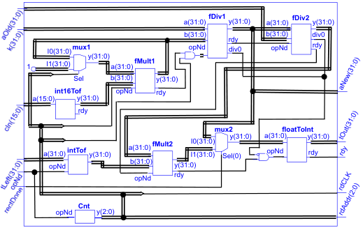
Fig. 5 shows the hardware logic layout for computing the reaction-time schedules. The multiplication of the reactant concentrations is performed iteratively by a single floating-point multiplier only, because of restrictions in the amount of available logic on the XC6SLX9 chip. This means that we loose in parallelisation because we have limited the number of floating-point operations to two multiplications and two divisions for each time schedule computation.
IV Evaluation
In this section, we provide an evaluation of the chemical engine middleware platform based on our prototype implementation in the XILINX Spartan6 FPGA family. The objectives of this evaluation are
- •
to demonstrate the runtime programability on hardware of (chemical) algorithms to control network traffic dynamics
- •
to quantify the performance gains enabled by running CAs on hardware.
To keep the discussion focused on these evaluation objectives, and avoid introducing new algorithms, we present the experiments with the exemplary CA that has been used in our discussions until now. In Sect.V, we briefly report on experiments with other CAs and their applications.
IV-A Experiment setup
We used CAs to control the service process of the egress queue of a standard Linux host (Linux, Kernel 3.8.6), and thereby shape its outgoing traffic.
We employ the tc tool to isolate a class of traffic in a separate FIFO queue. The arrival process of that queue provided the input for the CA: for each enqueued packet, an amount of molecules corresponding to the number of bytes in the packet was added to an input species S in the chemical engine. On the other end, an output species P was “connected” to the service process of the queue: for each P-molecule produced, a fixed number of bytes were allowed to leave the queue; when there were enough molecules to match the byte-size of the packet at the front of the queue, the packet was dequeued and transmitted. In both cases, the molecules-to-bytes ratio was kept fixed at 1 mol/KB.
To interface the FPGA (LX9) board, where the chemical engine lies, with the queue management subsystem of the linux kernel, we used the Parapin kernel module. Parapin module allows the use of the PC’s parallel port as a custom I/O interface (i.e., allows handling interrupts at the port pins, and accessing directly the parallel port registers). We then wired one of LX9’s I/O connectors to the parallel port of the PC. With such an interfacing, it was possible to produce/process interrupts every 100 ns.
The results shown in the graphs that follow concern UDP traffic produced with the iperf tool (client side running on the controlled node). We have not included measurements with TCP traffic because there, effects of the CA controller are coupled with TCP’s control-loop behaviour, and thus are not easy to evaluate.
Fig. 6 shows the host-to-host topology of the experiment, over the high-speed switched network of the university.

IV-B Runtime programmability on hardware
To test and demonstrate the runtime programmability of CAs on the FPGA-embedded chemical engine, we first instantiated in the system a simple CA (Fig. 7) that paces packet transmissions by a variable time delay. The simple reaction network essentially imposes the LoMA (3) as a queue service policy. The CA “program” is essentially the following reaction network specification:
|
In the first of the experiment (see Fig. 8), the output rate followed the average load of the queue. At the same time the burstiness of the arrival process was smoothed out (filtering of high frequency components). The cut-off frequency for such a filtering was set via -coefficient (= s-1).

(a) System
(b) Reaction
After , we re-programmed the with Rnet1 (enzymatic rate controller – see Fig. 1), by loading the following CA specification:
|
Setting and s-1 fixed the rate cap at 0.5 Gbps.
In (see Fig. 8), a new round of UDP transmissions increased the load above the predefined rate cap. The output rate ramped-up to the cap rate, and remained at that limit until the transmission ended. A third round of UDP transmission started at time s. The load still had mixed high-frequency and low-frequency bursts, but this time did not exceed the rate cap. The CA worked as a pacer: the transmission rate followed closely the slow fluctuations of the arrival rate, but very high-frequencies were filtered out.
For the last part of the experiment, we updated the last CA specification, re-tuning its parameters so as to filter even more the traffic bursts (medium scale frequencies). To do so, we merely modified the values of individual registers without re-loading the entire specification (or involving changes in the bitstream). The modified parameters were s-1 (to reduce the filtering cut-off frequency), and Kmol (to maintain the rate cap at 0.5 Gbps, since ). Fig. 9 shows the difference in the output behaviour under the same arrival traffic pattern. The rate capping remained consistent (), while the smoothing of burstiness was more pronounced () when s-1.
In summary this experiment demonstrates both how new algorithms can be installed in the chemical engine, as well as how a CA can be fine-tuned by (re-)configuring its parameters. Both operations are possible at runtime.
IV-C Cost-savings from CAs on hardware
To quantify the advantage of an on-hardware execution of CAs, we looked at the computational cost involved when executing CAs in the linux kernel. The rationale behind this measurement is that this computational overhead/penalty disappears as soon as we move the CAs on the FPGA, and together with it any delays in packet transmissions due to system load.
We have employed the ChemFlow platform that was used in the experiments of [18, 19], and our metric has been the utilisation of the CPU when engaged in CA (algorithmic) computations only; omitting related management tasks (such as servicing of interrupts for the queue management operations, and monitoring of the chemical engine). To understand how the CPU load scales, we measured two CAs of different complexity, Rnet1 and Rnet2 (Rnet1 has double amount of species and reactions than Rnet2), and we also varied for each of them the input rate of events that they processed.
The results for both CAs are plotted in Fig. 10, grouped by the rate of input events. We can see that beyond a certain rate (1M mol/s) the cost increases dramatically, eventually stealing the CPU from other (application) tasks in the system. Thus, even simple CAs are computationally expensive! Doubling the amount of occupied chemical resources does not really double the load, but nevertheless increases it significantly ().
In the case of the on-hardware implementation, there still exists a saturation point where the input rate hits the limit of the FPGA clock. In our implementation, clocking the FPGA at 80 MHz and using 1 mol/KB resolution, this limit is approximately at 800 Mbps when two reactions are involved in the CA, and at 1.6 Gbps when there is one reaction involved. Even with such a low-end FPGA, today these effected speeds are well within norm for edge connectivity, access networks, and corporate LAN infrastructures (where traffic shaping is mostly needed). As we climb up the range of higher-end FPGAs and dedicated OS interfaces (e.g., PCIe bus), there is substantial improvement in performance (see Sect.V-D) that can serve application needs even deeper in the core of the network. Finally, the scaling of CAs’ complexity is not a problem in the case of on-hardware implementation thanks to parallelisation. The only limitation can be the size of the FPGA (in terms of number of cells).
V Discussion
To support our initial claim that CAs are well suited to develop a broad range of control functions for network dynamics, we start this section by providing a couple of algorithms related to queue scheduling and AQM (together with others already presented in past literature [16, 18, 19], they provide a comprehensive account for network dynamics functions that includes queuing disciplines, AQM, rate control, distributed access, traffic conditioning, distributed consensus, and flow control). We then discuss design extensions based on the OpenFlow architecture [21], to illustrate the actual contextualisation in SDN. We finish the discussion with a reference to tradeoffs and performance expectations of running the CA framework on various FPGA devices currently available on market.
V-A Chemical controllers for Active Queue Management (AQM)
A minimal extension of the enzymatic rate controller scheme in Fig. 1 suffices to turn the CA into an AQM scheme with packet dropping behaviour analogous to RED [65]. As shown in Fig. 11, the extension involves one additional reaction () and one species (D), whose concentration regulates the drop process at the head of the queue.
Reaction (much slower than ) occasionally “samples” the amount of enqueued packets awaiting transmission (i.e., concentration of species S). If the queue size starts growing (i.e., packets dequeued at too slow rate or the arrival rate is too high), accelerates fast (as a second order function of the queue size) creating drop tokens (D) to remove packets from the head of the queue. As the queue size decreases, quickly recovers again its low speed and effects on queue drops.
Fig. 12 validates experimentally this behaviour in a simple scenario where iperf-generated VBR UDP traffic goes through a queue controlled by this CA. The upper rate limit of the enzymatic controller was set to 0.4 Gbps, representing the maximum desired link utilisation (condition under which no queue is built-up). The UDP traffic was admitted to the queue initially at 0.2 Gbps and then at 1 Gbps, during different phases of the experiment (2s-13s and 14s-25s). One can see the drop rate (black line) being effectively zero under low-load conditions (first phase). As soon as the rate cap was reached, and the queue started building up (second phase), the drop-mechanism kicked in emptying the queue at a pace synchronised (no phase lag) with the queue size variations.
Note that while the CA operates on the queue size (S species), its configuration is in terms of throughput/latency cap (0.4 Gbps) at the queue! In fact, this is an intuitive/automated configuration approach sought in modern AQMs [6, 7].

(a) System
(b) Reaction set
V-B Chemical controllers for traffic prioritisation
By combining the distributed rate control scheme presented in [19] with the CA for AQM of the previous section, we are able to create a CA for weighted, or proportional, fair-queuing (Fig. 13). The servers of the participating queues in the scheme (typically corresponding to distinct classes of traffic) are controlled by identical reaction sub-networks, sharing their token/molecular state (aggregate of species feeds back to each ). Through coefficients at each sub-network, one can configure the proportional bandwidth shares for each queue. The outputs of these queues then aggregate at a single egress queue, which is controlled by the last stage of the CA, a sub-network implementing the AQM in Sect.V-A.
Without delving into analytical details due to space limitation,44 4 The analysis is a straightforward product of the theory in [18]. we show an experimental validation in Fig. 14. The service processes of three intermediate queues and the egress queue (where they aggregate) were controlled by the reaction network Rnet4. Fig. 14(a) shows the CBR admission rates of traffic, in two phases (s and s), to the three queues ( and flows had the same rate). Fig. 14(b/c/d) demonstrate fair-sharing and weighted (proportional) fair-sharing by means of different setting. In the first phase, the total aggregate admission rate (at the intermediate queues) did not exceed the configured 2Mbps-limit at the egress queue. All flows claimed and received what they needed from the available bandwidth. In the second phase, the total aggregate admission rate exceeded by far the rate limit and prioritisation kicked in. The share each flow received is (statistically) proportional to the weights expressed as parameters.
It is worth mentioning that CAs of this size become very fast prohibitive for execution in CPU at the host OS.

V-C CAs and Software Defined Networking

In the SDN research landscape deployment of CAs on hardware opens a door to programmable network dynamics. Looking at the OpenFlow (OF) [21] architecture as one of the reference enabling southbound technologies in SDN,55 5 We are not bound to OpenFlow as a southbound interface; our choice was driven by its extensibility, broad acceptance by hardware manufacturers, and its evolution as a melting pot for new features and capabilities. Fig. 15 illustrates how the integration of our chemical framework will be effected in an OF controlled switch.
The dark coloured (in blue) switch subsystems are those currently liable for remote configuration and re-programming via an OF controller.66 6 This holds until current version 1.4 of the OF protocol One can see that the queuing subsystem, although available for reading statistics through the OF protocol, cannot be remotely controlled or modified by an OF controller. Additionally, the only traffic shaping/management feature supported in this architecture is instantaneous per-flow rate policing. However, the OF architecture accounts already for more than 40 counters and meter bands (collecting state information and statistics), which is all a CA requires as inputs.
As shown in Fig. 15, an FPGA-based “chemical subsystem”, like the one presented in this paper, can be hosted at any OF switch on NetFPGA or other FPGA-enabled network cards, or on typical manufacturer-provided FPGA boards wired through hardware interrupts to the OS. Internally (horizontal interface), it should be “permanently” interfaced with the queuing subsystem; on one side controlling the enqueue, dequeue (queue server) and head-drop primitives, and on the other side controlling the increment/decrement primitives of dedicated I/O species (registers). In a similar fashion, it can also be “non-permanently” (programmatically/on-demand) interfaced with the counter-set of the OF-switch which may be used as additional input species. These are all mere interrupt signals.
Remote access (southbound SDN interface) from an OF controller is effected through the OF protocol’s experimental extensions. Very simple primitives as in [66] can provide admission control of the chemical engines, as well as loading and reseting of algorithms by means of reaction network specifications (or partial specifications providing incremental updates and modifications for existing reaction networks).
V-D Which logic device?
For our experimentation we have used a low-end FPGA device (XC6SLX9, the 2nd smallest device of the Spartan-6 family), in which we have exhausted most of the available logic (70% of slice LUTs) Yet, we were able to implement a powerful chemical engine that accommodates up to 255 species and up to 8 reactions, with a maximum of 8 reactant and product species (sufficient for a number of practical CAs). This implementation uses a single reaction scheduler (LoMA core) for all 8 reactions, which computes propensities through a linear pipeline of multiplier DSPs.
By using the XC7K325T FPGA, which is currently mounted on the popular NetFPGA-1G-CML board, any concern on logic resource exhaustion instantly vanishes: the same implementation of the chemical middleware framework with an instantiation of the same amount of chemical resources would utilise barely 1% of slice LUTs available. Indicatively, in Table III we provide summarised reports from the EDA software of Xilinx, for the amount of logic resources required on the XC7K325T FPGA, when instantiating different amounts of chemical resources in the chemical middleware (up to 256 species, reactions, 8 reactants and products, and a single LoMA core with a linear pipeline). While the size of the LoMA core is fixed (e.g., 722 Slices, 798 Slice Reg, 2334 LUTs, 79 LUTRAM, and 4 DSP48E1s on the XC7K325T FPGA), the logic utilisation scales up as a function of the maximum amount of chemical resources one is willing to make available in the system for CAs (e.g., number of reactions, of species, order etc.).
| = 2 | = 4 | = 8 | =32 | |
| # Slice Registers | 1’338 | 1’533 | 1’922 | 4’290 |
| # Slice LUTs | 3’071 | 3’464 | 3’931 | 7’838 |
| # Occupied Slices | 1’145 | 1’340 | 1’792 | 4’398 |
| # DSP48E1s | 4 | 4 | 4 | 4 |
Next, our system implementation is optimised for economy in logic resources, at the cost of speed. Operationally, it has been tested at 40 and 80 MHz but it can also work at 160 MHz, and with optimising differently the circuitry it would be possible to use at 320 MHz.77 7 The presets of 40, 80, 160 or 320 MHz are the allowed clocking frequencies of the XC6SLX9 FPGA, as specified by the manufacturer. At 40 MHz and 80 MHz clock, the system can process external events (e.g. packet arrivals) that occur every 10 s and 5 s respectively (and would be capable of handling 2.5 s with 160 MHz clock and down to 1.2 s with a 320 MHz clock). Moreover, it is able to process correctly two sporadic events occurring 50 ns apart, so long as they last at least ns each. FPGAs with higher clocking frequencies would provide even better resolution, e.g. the XC7K325T-2 FPGA with up to 650 MHz clocking frequency would allow down to 615 ns resolution. Overall, higher clocking frequency means implementing the the LoMA core with faster DSP modules.
Given a certain FPGA, one can further optimise for speed, at the cost of logic resource economy, by improving drastically on parallelisation. First, one can employ multiple LoMA cores (up to dedicating one to each reaction). Second, one can employ in the design of the LoMA core a logarithmic pipeline of DSPs (for the computation of propensities). We have experimented with such a design on the XC7K325T-2 FPGA. By dedicating a LoMA core to each reaction in the configuration of column 4 in Table III, the number of clk-cycles for re-scheduling the reactions dropped from 1600 to 52, while the logic resource budget increased to 30’055 slice registers, 79’016 slice LUTs, and 128 DSP48E1s. By additionally changing the pipeline of the LoMA core, we attained a further reduction to only 24 clk-cycles, and a further increase in logic consumption to 54’154 slice registers, 113’495 slice LUTs, and 320 DSP48E1s. This is still less than 50% of the logic resources available on the XC7K325T-2 FPGA, and with a clocking frequency of 400 MHz we have an impressive 60 ns resolution.
At this point however, it is worth noting that these improvements on speed do not necessarily imply better algorithmic performance. Since the hosted CAs are dynamical systems there is always a performance trade-off for each CA between speed of convergence and region of stability, and the choice is application specific (see [18] for details).
VI Conclusion
We have introduced, implemented and evaluated a framework that enables run-time (re-)programmable algorithms on FPGA hardware. These algorithms, which are inspired and based on laws and principles of Chemistry, are particularly suited to functions featuring control of network dynamics.
The very simple high-level representation of these algorithms (as chemical reaction networks)
- •
has allowed the expression of accurate mathematical models directly on hardware without the need for low-level HDL programming or even finite state automata,
- •
leads to fully parallelisable implementations, where parts of an algorithm can be modified separately and independently of the rest of the program,
- •
has enabled their programmability and configurability on hardware at sub-second latencies and without the need to field re-program FPGAs.
While functions for network dynamics is merely our playground, these algorithms may describe also user application logic, performing calculations for datasets other than packets in queues. Hence, in our understanding, this work entails a promising prospect for on-demand offloading general numerical logic directly on FPGA hardware, previously only flexibly expressed at the application level and within the overheads of an operating system. This obsoletes the need for the less performance- and power-efficient VonNeumman-architecture-based CPUs and GPUs.
References
- [1] M. Alizadeh, A. Kabbani, T. Edsall, B. Prabhakara, A. Vahdat, and M. Yasuda, “Less is more: Trading a little bandwidth for ultra-low latency in the data center,” in Proc. of the USENIX Conference on Networked Systems Design and Implementation, San Jose (CA), USA, Apr 2012, pp. 19–19.
- [2] M. Alizadeh, A. Greenberg, D. A. Maltz, J. Padhye, P. Patel, B. Prabhakar, S. Sengupta, and M. Sridharan, “Data center TCP (DCTCP),” in ACM SIGCOMM Computer Comm. Review, vol. 40, no. 4, Oct 2010, pp. 63–74.
- [3] H. Rodrigues, J. R. Santos, Y. Turner, P. Soares, and D. Guedes, “Gatekeeper: Supporting bandwidth guarantees for multi-tenant datacenter networks,” in Proc. of the USENIX Workshop on I/O Virtualization (WIOV), Portland (OR), USA, Jun 2011.
- [4] V. Jeyakumar, M. Alizadeh, D. Mazières, B. Prabhakar, C. Kim, and A. Greenberg, “EyeQ: practical network performance isolation at the edge,” in Proc. of the USENIX Conference on Networked Systems Design and Implementation, Lombard (IL), USA, Apr 2013, pp. 297–312.
- [5] H. Ballani, P. Costa, T. Karagiannis, and A. Rowstron, “Towards predictable datacenter networks,” in Proc. of the ACM SIGCOMM, Aug 2011, pp. 242–253.
- [6] K. Nichols and V. Jacobson, “Controlling queue delay,” in Magazine Communications of the ACM, vol. 55, no. 7, May 2012, pp. 42–50.
- [7] R. Pan, P. Natarajan, C. Piglione, M. S. Prabhu, V. Subramanian, F. Baker, and B. VerSteeg, “PIE: A lightweight control scheme to address the bufferbloat problem,” Draft Standard 00 draft-pan-aqm-pie, Internet Engineering Task Force (IETF), Dec 2012.
- [8] E. Thereska, H. Ballani, G. O’Shea, T. Karagiannis, A. Rowstron, T. Talpey, R. Black, and T. Zhu, “IOFlow: A software-defined storage architecture,” in Proc. of the ACM Symposium on Operating Systems Principles (SOSP), Farmington (PA), USA, Nov 2013, pp. 182–196.
- [9] Xilinx Inc., “Software defined specification environment for networking (SDNet),” White Paper, 2014.
- [10] P. Bosshart, D. Daly, G. Gibb, M. Izzard, N. McKeown, J. Rexford, C. Schlesinger, D. Talayco, A. Vahdat, G. Varghese, and D. Walker, “P4: Programming protocol-independent packet processors,” ACM SIGCOMM Computer Comm. Review, vol. 4, no. 3, pp. 87–95, Jul 2014.
- [11] V. Jeyakumar, M. Alizadeh, Y. Geng, C. Kim, and D. Mazières, “Millions of little minions: using packets for low latency network programming and visibility,” in Proc. of the ACM SIGCOMM, Chicago (IL), USA, Aug 2014, pp. 3–14.
- [12] P. Bosshart, G. Gibb, H.-S. Kim, G. Varghese, N. McKeown, M. Izzard, F. Mujica, and M. Horowitz, “Forwarding metamorphosis: fast programmable match-action processing in hardware for SDN,” in Proc. of the ACM SIGCOMM, Hong Kong, P.R.C., Aug 2013, pp. 99–110.
- [13] R. Ozdag, “Intel® Ethernet switch FM6000 series - software defined networking,” White Paper, 2012.
- [14] M. Kuhlewind, D. Wagner, J. M. R. Espinosa, and B. Briscoe, “Immediate ECN,” IETF-88 TSVAREA, Nov 2013.
- [15] T. Meyer and C. F. Tschudin, “Chemical networking protocols,” in Proc. of the ACM Workshop on Hot Topics in Networks (HotNets), New York (NY), USA, Oct 2009.
- [16] M. Monti, L. Sanguinetti, C. F. Tschudin, and M. Luise, “A chemistry-inspired framework for achieving consensus in wireless sensor networks,” in IEEE Sensors Journal, vol. 14, no. 2, Feb 2014, pp. 371–382.
- [17] T. Meyer and C. F. Tschudin, “A theory of packet flows based on law-of-mass-action scheduling,” in Proc. of the IEEE Int’l Symposium on Reliable Distributed Systems (SRDS), Irvine (CA), USA, Oct 2012.
- [18] M. Monti, T. Meyer, C. F. Tschudin, and M. Luise, “Stability and sensitivity analysis of traffic-shaping algorithms inspired by chemical engineering,” in IEEE Journal on Selected Areas of Communications (JSAC), vol. 31, no. 6, Jun 2013, pp. 1–11.
- [19] M. Monti, M. Sifalakis, T. Meyer, C. F. Tschudin, and M. Luise, “A chemical-inspired approach to design distributed rate controllers for packet networks,” in Proc. of the IFIP/IEEE-IM Workshop on Distributed Autonomous Network Management Systems (DANMS), Ghent, Belgium, May 2013.
- [20] M. Monti, P. Imai, and C. F. Tschudin, “Designing run-time environments to have predefined global dynamics,” in International Journal of Computer Networks and Communications (IJCNC), vol. 5, no. 3, May 2013, pp. 1–16.
- [21] N. McKeown, G. Parulkar, T. Anderson, L. Peterson, H. Balakrishnan, J. Rexford, S. Shenker, and J. Turner, “OpenFlow: Enabling innovation in campus networks,” ONF White Paper, Mar 2008.
- [22] J. W. Lockwood, N. McKeown, G. Watson, G. Gibb, P. Hartke, J. Naous, R. Raghuraman, and J. Luo, “NetFPGA – an open platform for gigabit-rate network switching and routing,” in Proc. of the IEEE Intl Conference on Microelectronic Systems Education (MSE), San Diego (CA), USA, Jun 2007, pp. 160–161.
- [23] J. Auerbach, D. F. Bacon, I. Burcea, P. Cheng, S. J. Fink, R. Rabbah, and S. Shukla, “A compiler and runtime for heterogeneous computing,” in Proc. of ACM/EDAC/IEEE Design Automation Conference (DAC), Jun 2012, pp. 271–276.
- [24] IEEE Computer Society, “IEEE standard VHDL language reference manual,” IEEE Standard 1076-2008, Jan 2009.
- [25] ——, “IEEE standard for Verilog hardware description language,” IEEE Standard 1364-2005, Apr 2006.
- [26] N. Possley, “Traffic management in Xilinx FPGAs,” Xilinx White Paper WP244 (v1.0), Apr 2006.
- [27] Altera Corp., “Enabling 100G traffic management,” http://www.altera.com/end-markets/wireline/applications/traffic/wil-traffic.html, Jan 2014.
- [28] Lattice Semiconductor Corporation, “Lattice announces low cost programmable SPI-4.2 solution,” http://ir.latticesemi.com/phoenix.zhtml?c=117422&p=irol-newsArticle&ID=1472678&highlight, Jan 2014.
- [29] M. Alizadeh, B. Atikoglu, A. Kabbani, A. Lakshmikantha, R. P. B. Prabhakar, and M. Seaman, “Data center transport mechanisms: Congestion control theory and IEEE standardization,” in Proc. of the Annual Allerton Conference on Communication, Control, and Computing, Monticello (IL), USA, Sep 2008, pp. 1270–1277.
- [30] N. Dukkipati, G. Gibb, and J. Z. Nick McKeown, “Building a RCP (rate control protocol) test network,” in Proc. of the IEEE Annual Symposium on High-Performance Interconnects, Stanford (CA), USA, Aug 2007, pp. 91–98.
- [31] N. Malangadan and G. Raina, “Rate based feedback: some experimental evaluation with NetFPGA,” in Proc. of the IEEE International Conference on Communication (ICC), Kyoto, Japan, Jun 2011, pp. 1–6.
- [32] S. Y. Hanay, A. Dwaraki, and T. Wolf, “High-performance implementation of in-network traffic pacing,” in Proc. of the IEEE International Conference on High Performance Switching and Routing (HPSR), Cartagena, Spain, Jul 2011, pp. 9–15.
- [33] G. Chen, “A short historical survey of functional hardware languages,” ISRN Electronics, vol. 2012, pp. 1–11, 2012.
- [34] D. F. Bacon, R. Rabbah, and S. Shukla, “FPGA programming for the masses,” ACM Queue, vol. 11, February 2013.
- [35] R. S. Nikhil, “Abstraction in hardware system design,” ACM Queue, vol. 9, 2011.
- [36] J. Cardoso and P. Diniz, Compilation techniques for reconfigurable architectures. Springer, 2009.
- [37] P. Coussy and A. Morawiec, High-level synthesis: from algorithm to digital circuit. Springer, 2008.
- [38] D. O’Loughlin, A. Coffey, F. Callaly, D. Lyons, and F. Morgan, “Xilinx Vivado high level synthesis: Case studies,” in Proc. of Irish Signals Systems Conference 2014 and 2014 China-Ireland International Conference on Information and Communications Technologies (ISSC 2014/CIICT 2014)., Jun 2014, pp. 352–356.
- [39] P. J a askel ainen, C. de la Lama, P. Huerta, and J. Takala, “OpenCL – based design methodology for application-specific processors,” in Proc. of the IEEE International Conference Embedded Computer Systems (SAMOS), Samos, Greece, Jul 2010, pp. 223–230.
- [40] A. Papakonstantinou, K. Gururaj, J. Stratton, D. Chen, J. Cong, and W.-M. Hwu, “FCUDA: Enabling efficient compilation of CUDA kernels onto FPGAs,” in Proc. of IEEE Symposium onApplication Specific Processors (SASP), 2009, San Francisco (CA), USA, Jul 2009, pp. 35–42.
- [41] J. Auerbach, D. F. Bacon, P. Cheng, and R. Rabbah, “Lime: A Java-compatible and synthesizable language for heterogeneous architectures,” SIGPLAN Not., vol. 45, no. 10, pp. 89–108, Oct 2010.
- [42] J. Bachrach, H. Vo, B. Richards, Y. Lee, A. Waterman, R. Aviẑienis, J. Wawrzynek, and K. Asanović, “Chisel: Constructing hardware in a scala embedded language,” in Proc. of the ACM/EDAC/IEEE Design Automation Conference (DAC), Jun 2012, pp. 1212 – 1221.
- [43] D. Greaves and S. Singh, “Designing application specific circuits with concurrent C# programs,” in proc of. IEEE/ACM International Conference on Formal Methods and Models for Codesign (MEMOCODE), Grenoble, France, Jul 2010, pp. 21–30.
- [44] S. Singh, “A demonstration of co-design and co-verification in a synchronous language,” in Proc. of the Design, Automation and Test in Europe Conference and Exhibition, vol. 2, Feb 2004, pp. 1394–1395.
- [45] C. Dase, J. Falcon, and B. MacCleery, “Motorcycle control prototyping using an FPGA-based embedded control system,” Control Systems, IEEE, vol. 26, no. 5, pp. 17–21, Oct 2006.
- [46] T. Meyer, “On chemical and self-healing networking protocols,” Ph.D. Dissertation, Faculty of Computer Science, University of Basel, Switzerland, 2011.
- [47] S. Stepney, “Nonclassical computation – a dynamical systems perspective,” in Handbook of Natural Computing, Springer, vol. 4, 2012, pp. 1979–2025.
- [48] P. Dittrich, “The bio-chemical information processing metaphor as a programming paradigm for organic computing,” in Proc. of the Workshop Self-Organization and Emergence, Conference on Architecture of Computing Systems (ARCS), Innsbruck, Austria, Mar 2005, pp. 95–100.
- [49] J. Banâtre, P. Fradet, and Y. Radenac, “Principles of chemical programming,” in Electronic Notes in Theoretical Computer Science, Elsevir, vol. 124, no. 1, Mar 2005, pp. 133–147.
- [50] G. Paŭn, “Computing with membranes,” in Journal of Computer and System Sciences, vol. 61, no. 1, 2000, pp. 108–143.
- [51] W. Banzhaf, P. Dittrich, and H. Rauhe, “Emergent computation by catalytic reactions,” in Nanotechnology 7 (1996) 307–314, vol. 7, no. 4, Dec 1996, pp. 307–314.
- [52] J. Giavitto and O. Michel, “MGS: a rule-based programming language for complex objects and collections,” in Electronic Notes in Theoretical Computer Science, Elsevir, vol. 59, no. 4, Nov 2001, pp. 286–304.
- [53] N. Matsumaru, P. Kreyssig, and P. Dittrich, “Organisation-oriented chemical programming,” in Organic Computing – A Paradigm Shift for Complex Systems Autonomic Systems, vol. 1, 2011, pp. 207–220.
- [54] M. Viroli, M. Casadei, S. Montagna, and F. Zambonelli, “Spatial coordination of pervasive services through chemical-inspired tuple spaces,” in Journal ACM Transactions on Autonomous and Adaptive Systems (TAAS), vol. 6, no. 2, Jun 2011, pp. 14:1–14:24.
- [55] C. D. Napoli, M. Giordano, Z. Németh, and N. Tonellotto, “Using chemical reactions to model service composition,” in Proc. of the ACM International Workshop on Self-Organizing Architectures, Washington (DC), USA, Jun 2010, pp. 1–8.
- [56] F. Horn and R. Jackson, “General mass action kinetics,” Archive for Rational Mechanics and Analysis, vol. 47, no. 2, pp. 81–116, 1972.
- [57] O. Wolkenhauer, M. Ullah, W. Kolch, and K. Cho, “Modeling and simulation of intracellular dynamics: Choosing an appropriate framework,” in IEEE Transactions on Nanobioscience, vol. 3, no. 3, Sep 2004, pp. 200–207.
- [58] H. M. Sauro and B. Ingalls, “Conservation analysis in biochemical networks: computational issues for software writers,” Biophys. Chem., vol. 109, no. 1, pp. 1–15, Apr 2004.
- [59] M. Monti and M. Sifalakis, “Extending the artificial chemistry to design networking algorithms with controllable dynamics,” Technical Report CS-2012-003, Univ. of Basel, Switzerland, http://cn.cs.unibas.ch/pub/doc/cs-2012-003.pdf, Jul 2012.
- [60] P. Dittrich, J. Ziegler, and W. Banzhaf, “Artificial chemistries – a review,” in Artificial Life, vol. 7, 2001, pp. 225–275.
- [61] Xilinx Inc., “Spartan-6 family overview,” Product Specifications DS160 (v2.0), Oct 2011.
- [62] Avnet Inc., “Xilinx Spartan-6 FPGA LX9 microboard,” User Guide, Rev C, Aug 2011.
- [63] Xilinx Inc., “LogiCORE IP floating-point operator v6.0,” Application Note DS816, Jan 2012.
- [64] IEEE, “IEEE standard for floating-point arithmetic,” IEEE Std 754 - 2008 (revision IEEE Std 754 - 1985), 2008.
- [65] S. Floyd and V. Jacobson, “Random early detection gateways for congestion avoidance,” IEEE/ACM Transactions on Networking, vol. 1, no. 4, pp. 397–413, Aug 1993.
- [66] M. Sifalakis, S. Schmid, T. Chart, and D. Hutchison, “A generic active service deployment protocol,” in Proc. of the International Workshop on Active Network Technologies and Applications, Osaka, Japan, May 2003, pp. 100–111.