Dangerous connections: on binding site models of infectious disease dynamics

As in our earlier paper (Leung et al., 2015), our model formulation is in the tradition of physiologically structured population models (PSPM (Metz and Diekmann, 1986; Diekmann et al., 1998b; Diekmann et al., 2001)). This means that we start from the notion of state at the individual level, called i-state (where i stands for individual). Model specification involves, first of all, a description of changes in time of the i-state as influenced by i-state itself and the relevant environmental variables that capture the influence of the outside world. Next the model specifies the impact of individuals on the environmental variables. Thus the feedback loop that creates density dependence, i.e. dependence among individuals, is described in a two step procedure. To lift the i-level model to the population level (p-level) is just a matter of bookkeeping, see Diekmann and Metz (2010) for a recent account.

In the setting considered here, i-state ranges over a finite set. As a consequence, the p-level equations are ordinary differential equations (ODE). These ODE describe, apart from death and birth of individuals, the dynamical changes of i-state, i.e. how individuals jump back and forth between the various states. In the spirit of the theory of Markov chains (Taylor and Karlin, 1998), we describe an individual not by its actual state but by the probability distribution, i.e. the probability of being in the various states. Equating a p-level fraction to an i-level probability provides the link between the two levels.

The approach of both earlier work and this paper is to pretend that the label can be considered as the i-state, the information about the individual that is relevant for predicting its future. The i-state contains information about partners, but not about partners of partners. Implicitly this entails that we use a mean field description of partners of partners. We call this the ‘mean field at distance one’ assumption. The description of partners of partners is incorporated in an environmental variable, the information about the ‘outside world’ that is relevant for a prediction of the future of the individual.

A rather special feature of the models considered here is that i-state involves a number of conditionally independent components: the binding sites. An individual has binding sites for partners. Two free binding sites can be joined together to form a partnership between two individuals (see Fig. 1 for an illustration). In graph theory the words ‘half-edge’ or ‘stub’ are often used. We think that for static networks these terms capture the essence much better than the word ‘binding site’. But the latter provides, in our opinion, a better description for dynamic networks. The fact that our research started with dynamic networks is responsible for our choice of terminology.

It is attractive to model the dynamics of one binding site and next use combinatorics to describe the full i-state. It is precisely this aspect that we did not yet elaborate in Leung et al. (2015) but highlight now. It is precisely this aspect that uncovers the link/relationship between the work of Lindquist et al. (2011); Leung et al. (2015) on the one hand and the edge-based modelling approach of Volz, Miller and co-workers (Volz and Meyers, 2007; Volz, 2008; Volz and Meyers, 2009; Miller et al., 2012; Miller and Volz, 2013) on the other hand.

Volz and Miller focus on the binding site (=half-edge/stub) and individual level and draw p-level conclusions by a clever use of probabilistic arguments to determine the relevant environmental variables. Lindquist et al. (2011) systematically formulate and analyse the p-level equations. In Leung et al. (2015) we too emphasized the p-level equations, but used the i-level version to derive an expression for $R_{0}$. The link between the two was established by somewhat contrived linear algebra arguments. In the present paper we build our way upwards from binding site - via individual - to population level. One of the secondary aims of this paper is to show that the systematic methodology of PSPM is also very useful when i-state space is discrete, rather than a continuum, and when i-state involves multiple identical components.

Now, consider a network. An epidemic starts when, at some point in time, a small fraction of the population is infected from outside. Our idealized description shifts the ‘point in time’ towards $-\infty$ while letting the fraction become smaller and smaller. In other words, our story starts ‘far back’ in time when all individuals are still susceptible (see Appendix A for elucidation). We consider three different situations, characterized by the relation between the time scales of, respectively, transmission, partnership dynamics and demographic turnover:

• I

  The disease dynamics are fast relative to any partnership- or demographic changes. The network is static and everyone is susceptible at time $t=-\infty$.

• II

  The disease dynamics are on the same time scale as the partnership dynamics, but fast relative to demographic turnover. In this network individuals can acquire and lose partners over time. Everyone is susceptible at time $t=-\infty$.

• III

  The disease dynamics and partnership- and demographic changes are on the same time scale. Here the age of an individual matters and we assume that, at birth, an individual enters the population as a susceptible without any partners.

We assume that infection is transmitted from an infectious individual to a susceptible partner at rate $\beta$ and infectious individuals recover at rate $\gamma$ (but see Section 2.5 for a far more general setting). We also assume that infection does not influence the partnership dynamics or the probability per unit of time of dying in any way.

Each individual in the population is assumed to have a so-called partnership capacity $n$ which denotes the number of binding sites it has (so $n$ is the maximum number of simultaneous partners it may have). Throughout the life of the individual this partnership capacity does not change. An individual with partnership capacity $n$ can be thought of as having $n$ binding sites for partners (in Fig. 1, individuals $u$, $v$, and $w$ have partnership capacities 4, 3, and 2, respectively). We call the individual to which a binding site belongs its owner. For the purpose of this paper, we will assume that all individuals have the same partnership capacity $n$. One can easily generalize this by allowing individuals to have different partnership capacities; in that case, one only needs to average over $n$ in the correct way (see Section 2.5 for the static case).

An individual with partnership capacity $n$ is to some extent just a collection of $n$ binding sites. These $n$ binding sites are coupled through the disease status (or death) of their owner. We assume that this is the only manner in which the binding sites of an individual are coupled. As long as the disease status of the owner does not change (and the owner does not die), binding sites behave independently of one another and the ‘rules’ for changes in binding site states are the same for each binding site. Obviously the latter depends on the network dynamics under consideration (either case I, II, or III). As a port to the world, a binding site can be in one of four states:

• •

  0 - free

• •

  1 - occupied by a susceptible partner

• •

  2 - occupied by an infectious partner

• •

  3 - occupied by a recovered partner.

Here (and in the remainder of this introduction) our formulation is precise for case II while sometimes requiring minor adaptations to capture cases I and III.

A key component of the model is the description of the dynamics of a binding site. The state of an individual is specified by listing its disease status and the states of each of its $n$ binding sites. So it makes sense to first consider a binding site as a separate and independent entity and to only take the dependence (by way of a change in the disease status of the owner) into account when we combine $n$ binding sites into one individual.

The case of a susceptible binding site (i.e. a binding site with a susceptible owner) is, as will become clear, far more important than the other cases. This is partly due to our assumption that all individuals start out susceptible, i.e. are susceptible at time $t=-\infty$ (I and II) or at birth (III). The dynamics of a susceptible binding site are described by a differential equation for the variable $x(t)=(x_{i}(t))$, $i=0,1,2,3$. Here $x_{i}$ can be interpreted as the probability that a binding site is susceptible and has state $i$ at time $t$, given that its owner does not become infected through one of its other $n-1$ binding sites (in other words, by conditioning on the individual not getting infected through its $n-1$ other binding sites, the only way the individual could get infected is through the binding site under consideration). In particular, given that its owner does not become infected through one of its other binding sites,

$$\bar{x}(t)=x_{0}(t)+x_{1}(t)+x_{2}(t)+x_{3}(t)$$

(1.1)

is the probability that the binding site is susceptible at time $t$ (or, in other words, that the owner is not infected along this binding site before time $t$). Accordingly, the probability that an individual is susceptible at time $t$ is equal to

$$\bar{x}(t)^{n}.$$

(1.2)

In order to arrive at a closed system of equations for $x$, we need to go through several steps. The variable $x$ contains information about a partner. Consequently the dynamics of $x$ is partly determined by partners of partners, hence by one or more environmental variables. The ‘mean field at distance one’ assumption yields expressions for environmental variables in terms of subpopulation sizes (for a given label, the corresponding subpopulation size is the fraction of the population that carries this label). In turn, p-level fractions can be expressed in terms of i-level probabilities. And since a susceptible individual is in essence a collection of $n$ conditionally i.i.d. binding sites, we can use combinatorics to express i-level probabilities in terms of binding-site-level probabilities as incorporated in $x$.

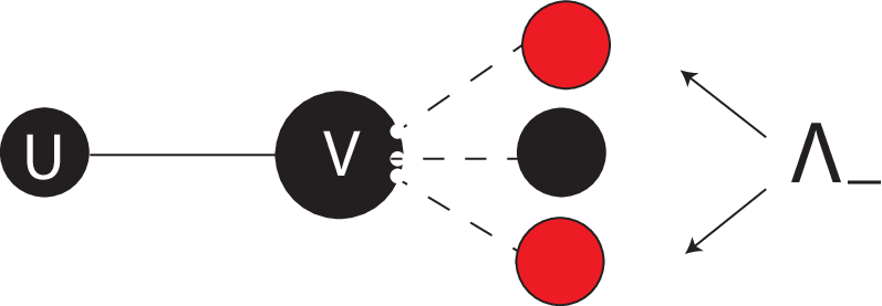
The exchangeability of the binding sites is broken by the infection event. There is exactly one binding site along which infection took place, viz. the binding site occupied by the individual’s epidemiological parent, and for this binding site we know with certainty that it is in state 2 at time of infection $t_{+}$. We call the binding site through which the change in the owner’s disease status occurred the ‘exceptional’ binding site. The other $n-1$ binding sites are i.i.d. and, at time $t_{+}$, they are distributed according to $x(t_{+})$. Recovery (and death) is an event that occurs at a constant rate for an infectious individual so independent of binding site states. Therefore, also after recovery, there remains exactly one exceptional binding site, viz. the one through which transmission occurred. See also Fig. 2 for an illustration of the exceptional binding site.

In Sections 2, 3, and 4 below, we will discuss the three network model cases I, II, and III separately. For each of the three cases we will explain how the model can be formulated and described in terms of susceptible binding sites. By considering the susceptible binding site perspective we can write a closed system of only a few equations that fully determine the dynamics of i-level probabilities and p-level fractions. This system is then used to determine epidemiological quantities of interest: $R_{0}$, $r$, the final size (in cases I and II), and the endemic steady state (in case III). In all three cases, an explicit expression can be given for $R_{0}$. In case I, one can derive a simple scalar equation for the final size. In cases II and III, we could only implicitly characterize the final size and endemic equilibrium, respectively.

In Section 2 case I of a static network is considered. This is the simplest case among the three. The relative simplicity allows for the derivation of an ODE system for susceptible binding sites directly from the interpretation. This will be the first way in which we formulate the model for this case. But case I will also serve to illustrate the systematic procedure for model formulation in the spirit of PSPM. This systematic procedure allows us to connect the three different levels, viz. (1) binding sites, (2) individuals, and (3) the population, to each other.

In network case I, since it is relatively simple, one can derive a one-dimensional renewal equation from which $R_{0}$, $r$, and the final size almost immediately follow. This renewal equation will be treated in Section 2.5 for a much more general class of infectious disease models than only SIR.

Part of the systematic procedure in cases II and III focuses on infectious binding sites. We use case I to illustrate the model formulation concerning infectious (and recovered) binding sites, even though, for case I these are not needed to obtain a closed system for susceptible binding sites. However, depending on the network features of interest (e.g. fractions of infectious individuals) one may still want to consider infectious (and recovered) binding sites.

In network cases II and III, there are also network dynamics in absence of infection due to partnership changes (and demographic changes). We will only describe the essential characteristics of the network dynamics that we use in this paper. Certainly, much more can be said about the networks in absence of infection (Leung et al., 2012).

Finally, in Section 5 we discuss the issues that we have encountered in the three different network cases and pose some open problems. We end the discussion by considering a few generalizations that can easily be implemented using the systematic model formulation of Section 2.2.

We derive a closed system of ODE for $x$ purely on the basis of the interpretation of binding sites (without explicitly taking into account i-level probabilities or p-level fractions). The relatively simple setting of a static network allows us to do so. We are able to consider a binding site as a separate and independent entity all throughout its susceptible life. Implicitly, this uses (2.8) below. One can show that the system of ODE for $x$ indeed captures the appropriate large population limit of a stochastic SIR epidemic on a configuration network. This requires quite some work; see (Decreusefond et al., 2012; Barbour and Reinert, 2013; Janson et al., 2014).

Consider a susceptible binding site and assume its owner does not become infected through one of its other $n-1$ binding sites for the period under consideration. If a susceptible binding site is in state 2, it can become infected by the corresponding infectious partner. This happens at rate $\beta$ and when it happens, the binding site is no longer susceptible so it ‘leaves’ the $x$-system. It is also possible that the infectious partner recovers. This happens at rate $\gamma$. Finally, there is the possibility that a susceptible partner of a susceptible binding site becomes infectious (corresponding to a transition from state 1 to state 2). The rate at which this occurs depends on the number of infectious partners that this susceptible partner has. So here we use the mean field at distance one assumption: we average over all possibilities at the p-level to obtain one rate at which a susceptible partner of a susceptible binding site becomes infected. More specifically, we assume that there is a rate $\beta\Lambda_{-}(t)$ at which a susceptible partner of a susceptible binding site becomes infected at time $t$. Here $\Lambda_{-}(t)$ has the interpretation of the expected number of infectious partners of a susceptible partner of a susceptible individual.

Then, putting together the various assumptions described above, the dynamics of $x$ is governed by the following system (please note that the environmental variable $\Lambda_{-}$ is a p-level quantity that we have yet to specify):

$\displaystyle\frac{dx(t)}{dt}$

$\displaystyle=M\big(\Lambda_{-}(t)\big)x(t),$

(2.1)

with ‘far past’ conditions

$\displaystyle x_{1}(-\infty)$

$\displaystyle=1,\quad x_{2}(-\infty)=0=x_{3}(-\infty),$

and

$\displaystyle M(\Lambda_{-})$

$\displaystyle=\begin{pmatrix}-\beta\Lambda_{-}&0&0\\ \beta\Lambda_{-}&-(\beta+\gamma)&0\\ 0&\gamma&0\end{pmatrix}.$

(2.2)

To express $\Lambda_{-}$ in terms of $x$ we use the interpretation. Consider a susceptible partner $v$ of a susceptible individual $u$. Then, since $u$ is susceptible, we know that $v$ has at most $n-1$ binding sites that are possibly in state 2 (i.e. occupied by infectious partners). Since $v$ is known to be susceptible, also all its binding sites are susceptible (in the sense that their owner $v$ is). The probability that a binding site is susceptible at time $t$ is $\bar{x}$ with

$$\bar{x}(t)=x_{1}(t)+x_{2}(t)+x_{3}(t)$$

(2.3)

(recall (1.1) and note that in case I we have $x_{0}(t)=0$). The probability that a binding site is in state 2, given that the binding site is susceptible, is $x_{2}(t)/\bar{x}(t)$. Therefore,

$$\Lambda_{-}(t)=(n-1)\frac{x_{2}(t)}{\bar{x}(t)}.$$

(2.4)

By inserting (2.4) into (2.1) we find that the $x$-system is fully described by an ODE system in terms of the $x$-variables only:

	$\displaystyle x_{1}^{\prime}$	$\displaystyle=-\beta(n-1)\frac{x_{2}}{\bar{x}}x_{1}$		(2.5)
	$\displaystyle x_{2}^{\prime}$	$\displaystyle=\beta(n-1)\frac{x_{2}}{\bar{x}}x_{1}-(\beta+\gamma)x_{2}$
	$\displaystyle x_{3}^{\prime}$	$\displaystyle=\gamma x_{2},$

with ‘far past’ conditions

$$x_{1}(-\infty)=1,\quad x_{2}(-\infty)=0=x_{3}(-\infty).$$

Before analyzing (2.5) in the next section, we describe a systematic procedure, consisting of five steps, for deriving the complete model formulation. A key aim is to rederive the crucial relationship (2.4) in a manner that can be extended to the dynamic networks. Thus the present section serves to prepare for a quick and streamlined presentation of the cases II and III in Sections 3 and 4, respectively. The various steps reveal the relation between binding site probabilities, i-level probabilities and p-level fractions. In addition we introduce some notation.

In this section we consider the beginning and end of an epidemic. We first focus on $R_{0}$ and $r$, so on the start of an epidemic.

Note that we can very easily find an expression for $R_{0}$ from the interpretation: when infected individuals are rare, a newly infected individual has exactly $n-1$ susceptible partners. It infects one such partner before recovering from infection with probability $\beta/(\beta+\gamma)$. Therefore, the expected number of secondary infections caused by one newly infected individual is

$$R_{0}=\frac{\beta(n-1)}{\beta+\gamma}.$$

(2.9)

However, even though there should be no doubt about it, this does not yield a proof that this expression is indeed a threshold parameter with threshold value one for the stability of the disease free steady state of the p-level system. In order to provide a proof and to prepare for cases II and III, we now derive $R_{0}$ and $r$ from the binding site system (2.5).

Note that the p-level fractions $P_{(-,\boldsymbol{k})}(t)$ can be fully expressed in terms of the binding site level probabilities $x_{i}$ (eqs. (2.8) and (2.7)). Furthermore, the $P_{(-,\boldsymbol{k})}(t)$ fractions, i.e. the fractions concerning individuals with a $-$ disease status, form a closed system. Therefore, a threshold parameter for the disease free steady state of the binding-site system $x$ is also a threshold parameter for the disease free steady state of the p-level system. (This argument extends to the dynamic network cases II and III in Sections 3 and 4)

Linearization of system (2.5) in the disease free steady state $\tilde{x}_{1}=1$, $\tilde{x}_{2}=0=\tilde{x}_{3}$, yields a decoupled ODE for the linearization of the ODE for $x_{2}$. To avoid any confusion, let $\hat{x}_{2}$ denote the linearized $x_{2}$ variable. Then the linearization yields

$$\hat{x}_{2}^{\prime}=\beta(n-1)\hat{x}_{2}-(\beta+\gamma)\hat{x}_{2},$$

with ‘far past’ condition $\hat{x}_{2}(-\infty)=0$. In particular, the right-hand side of the ODE for $\hat{x}_{2}$ depends only on $\hat{x}_{2}$.

To illustrate the method used in case II and III in Sections 3.3 and 4.3, we derive expressions for $R_{0}$ and $r$ from a special form of the characteristic equation. Variation of constants for the ODE of $\hat{x}_{2}$ yields

$$\hat{x}_{2}(t)=\int_{0}^{\infty}e^{-(\beta+\gamma)\tau}\beta(n-1)\hat{x}_{2}(t-\tau)d\tau.$$

Substituting the ansatz $\hat{x}_{2}(t)=e^{\lambda t}$ yields the characteristic equation

$$1=\int_{0}^{\infty}\beta e^{-(\beta+\gamma)\tau}(n-1)e^{-\lambda\tau}d\tau.$$

Then there is a unique real root to this equation for $\lambda$ that we denote by $r$ and call the Malthusian parameter. Evaluating the integral we find that $r=\beta(n-1)-(\beta+\gamma)$. Likewise, we can derive the expression (2.9) for $R_{0}$ by evaluating the integral with $\lambda=0$.

Next, we consider the final size. We do so by considering the dynamics of $\bar{x}$ defined in (2.3). Recall (1.2), i.e. the probability that an individual is susceptible at time $t$, is given by $\bar{x}(t)^{n}$. We observe that, by (2.8), $\bar{x}(t)^{n}$ is also equal to the fraction of susceptible individuals in the population at time $t$. (Alternatively, one can show that $\sum_{\boldsymbol{k}}P_{(-,\boldsymbol{k})}(t)=\bar{x}(t)^{n}$ by combining (2.8) and (2.7).) In fact, it is possible to describe the dynamics of $\bar{x}$ in terms of only $\bar{x}$ itself. This was first observed in Miller (2011), where the Volz equations of (Volz, 2008) were taken as a starting point. The most important observation is the consistency relation

$$x_{1}=\bar{x}^{n-1}.$$

(2.10)

We can use the interpretation to derive (2.10); $x_{1}$ is the probability that a susceptible binding site with owner $u$ is occupied by a susceptible partner $v$, $\bar{x}^{n-1}$ is the probability that $v$ is susceptible given that it is a partner of a susceptible individual $u$ (see also (2.27) below).

Then, using (2.10) together with algebraic manipulation of the ODE system (2.5) (see (Miller, 2011) for details), one is able to find a decoupled equation for $\bar{x}$:

$$\bar{x}^{\prime}=\beta\bar{x}^{n-1}-(\beta+\gamma)\bar{x}+\gamma.$$

(2.11)

The fraction of susceptible individuals at the end of the outbreak is determined by the probability $\bar{x}(\infty)$. Since $\bar{x}$ satisfies (2.11) and $\bar{x}(\infty)$ is a constant, we find that necessarily $\bar{x}(\infty)$ is the unique solution in $(0,1)$ of

$$0=\beta\bar{x}(\infty)^{n-1}-(\beta+\gamma)\bar{x}(\infty)+\gamma$$

(2.12)

if $R_{0}>1$. The final size is given by

$$1-\bar{x}(\infty)^{n}.$$

In Section 2.5 we show that one can actually describe the dynamics of the probability $\bar{x}$ for deterministic epidemics on configuration networks for a much larger class of submodels for infectiousness. The SIR infection that we consider here is a very special case of the situation considered in Section 2.5. There we show that it is possible to derive a renewal equation for $\bar{x}$. The final size equation is then obtained by simply taking the limit $t\to\infty$. We highly recommend reading Section 2.5 to understand the derivation of the renewal equation for $\bar{x}$ based on the interpretation of the model (with a minimum of calculations).

In the preceding section we have seen that the $x$-system (2.5) for susceptible binding sites is all that is needed to determine several epidemiological quantities of immediate interest. On the other hand, we might not only be interested in the fraction (1.2) of susceptibles in the population, but also in the dynamics of i-level probabilities $p_{(d,\boldsymbol{k})}(t)$ (and likewise p-level fractions $P_{(d,\boldsymbol{k})}(t)$ given by (2.8)) for $d=+,\ast$.

So what happens after an individual becomes infected? We work out the details for infectious individuals and only briefly describe recovered individuals. Again, we are able to formulate the model following steps 1-5 of Section 2.2 (where the word ‘susceptible’ should be replaced by ‘infectious’ or ‘recovered’ whenever appropriate and step 3 should be replaced by a slightly different step 3’, but we will come back to this later on in this section). But now we need to take into account the exceptional binding site, i.e. the binding site through which infection was transmitted to the owner (see also Fig. 2).

In step 1 one considers the dynamics of infectious binding sites, i.e. binding sites having infectious owners. Suppose that the owner became infected at time $t_{+}$ and that it does not recover in the period under consideration. Let $y_{i}^{\text{e}}(t\mid t_{+})$ denote the probability for the exceptional binding site to be in state $i$ at time $t$, $i=1,2,3$. Similarly, $y_{i}(t\mid t_{+})$ denotes the probability for a non-exceptional binding site to be in state $i$ at time $t$, $i=1,2,3$. Here the probabilities are defined only for $t\geq t_{+}$. Note that $y$ and $y^{\text{e}}$ are probability vectors, i.e. the components are nonnegative and sum to one.

Instead of ‘far past’ conditions we now have to take into account the distribution of binding site states at time of infection $t_{+}$. Whether or not an infectious binding site is exceptional has an influence on the state it has at epidemiological birth. Indeed, the exceptional binding site is in state $2$ at time $t_{+}$ with probability 1, while the distribution of the state of a non-exceptional binding site at time $t_{+}$ is given by $x(t_{+})/\bar{x}(t_{+})$, i.e. we have boundary conditions

	$\displaystyle y_{1}^{\text{e}}(t_{+}\mid t_{+})$	$\displaystyle=0,$	$\displaystyle y_{1}(t_{+}\mid t_{+})$	$\displaystyle=x_{1}(t_{+})/\bar{x}(t_{+}),$		(2.13)
	$\displaystyle y^{\text{e}}_{2}(t_{+}\mid t_{+})$	$\displaystyle=1,$	$\displaystyle y_{2}(t_{+}\mid t_{+})$	$\displaystyle=x_{2}(t_{+})/\bar{x}(t_{+}),$
	$\displaystyle y^{\text{e}}_{3}(t_{+}\mid t_{+})$	$\displaystyle=0,$	$\displaystyle y_{3}(t_{+}\mid t_{+})$	$\displaystyle=x_{3}(t_{+})/\bar{x}(t_{+}).$

The mean field at distance one assumption again plays a role. Here, we need to deal with the environmental variable $\Lambda_{+}$ that is defined as the expected number of infectious partners of a susceptible partner of an infectious individual (see also Fig. 4 and compare with Fig. 3). We can redefine $\Lambda_{+}$ in terms of p-level fractions $P_{(-,\boldsymbol{k})}$ for susceptible individuals:

$$\Lambda_{+}(t)=\sum_{\boldsymbol{m}}m_{2}\frac{m_{2}P_{(-,\boldsymbol{m})}(t)}{\sum_{\boldsymbol{k}}k_{2}P_{(-,\boldsymbol{k})}(t)}.$$

(2.14)

In particular, once again, $\Lambda_{+}$ can be expressed in terms of $x$ by combining steps 2, 3, and 4. Using (2.14), (2.8), and (2.7) we find that

$$\Lambda_{+}(t)=1+(n-1)\frac{x_{2}(t)}{\bar{x}(t)}$$

(2.15)

(alternatively, one can find the same expression for $\Lambda_{+}$ in terms of $x$-probabilities directly from the interpretation, exactly as before in the case of $\Lambda_{-}$).

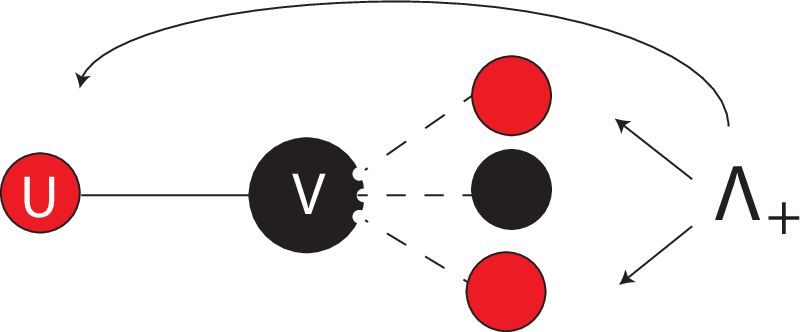
The rates at which changes in the states (1, 2, 3) of infectious binding sites occur is the same for each binding site, including the exceptional one. There is a rate $\gamma$ at which an infectious partner of an infectious binding site recovers (this corresponds to a change in state from 2 to 3). And there is a rate at which a susceptible partner of an infectious binding site becomes infected (either along the binding site under consideration or by one of its other infectious partners) corresponding to a change in state from 1 to 2. The rate at which this occurs is $\beta\Lambda_{+}$ where $\Lambda_{+}$ is defined by (2.14) and hence (2.15).

Recall that we condition on the infectious binding site under consideration not recovering, therefore, these are all state changes that can occur. So we find that the dynamics of $y$ and $y^{e}$ are described by the same ODE system

$\displaystyle\frac{dy(t\mid t_{+})}{dt}$

$\displaystyle=M_{+}\big(\Lambda_{+}(t)\big)y(t\mid t_{+}),$

(2.16)

with

$\displaystyle M_{+}(\Lambda_{+})$

$\displaystyle=\begin{pmatrix}-\beta\Lambda_{+}&0&0\\ \beta\Lambda_{+}&-\gamma&0\\ 0&\gamma&0\end{pmatrix},$

and case specific boundary conditions (2.13). Observe that this means that $y^{\text{e}}_{1}(t\mid t_{+})=0$ for all $t\geq t_{+}$.This also immediately follows from the interpretation: at time $t_{+}$, the binding site is occupied by an infectious partner, the network is static, and an infectious individual can not become susceptible again.

Next, we turn to infectious individuals. Compared to susceptible i-level probabilities, it is more involved to express infectious i-level probabilities in terms of $y^{\text{e}}$- and $y$-probabilities. Therefore, we first consider conditional i-level probabilities before finding an expression for the unconditional probabilities. We replace step 3 by step 3’.

So far we dealt with the SIR situation, where an individual becomes infectious immediately upon becoming infected and stays infectious for an exponentially distributed amount of time, with rate parameter $\gamma$, hence mean $\gamma^{-1}$. During the infectious period any susceptible partner is infected with rate (=probability per unit of time) $\beta$.

Here we incorporate randomness in infectiousness via a variable $\xi$ taking values in a set $\Omega$ according to a distribution specified by a measure $m$ on $\Omega$. This sounds abstract at first, but hopefully less so if we mention that the SIR situation corresponds to

	$\displaystyle\Omega$	$\displaystyle=(0,\infty),$
	$\displaystyle m(d\xi)$	$\displaystyle=\gamma e^{-\gamma\xi}d\xi,$

with $\xi$ corresponding to the length of the infectious period. In this section we only consider the setting where the ‘R’ characteristic holds, i.e. after becoming infected, individuals can not become susceptible for infection any more.

In order to describe how the probability of transmission to a susceptible partner depends on $\xi$, we need the auxiliary variable $\tau$ corresponding to the ‘age of infection’, i.e. the time on a clock that starts when an individual becomes infected. As a key model ingredient we introduce

$$\pi(\tau,\xi)=\text{the probability that transmission to a susceptible partner happens before $\tau$, given $\xi$}.$$

In the SIR example we have

$$\pi(\tau,\xi)=1-e^{-\beta\min(\tau,\xi)}.$$

It is important to note a certain asymmetry. On the one hand, there is dependence in the risk of infection of partners of an infectious individual $u$. Their risk of getting infected by $u$ depends on the length of the infectious period of $u$ (and, possibly, other aspects of infectiousness encoded in $\xi$). On the other hand, if $u$ is susceptible, the risk that $u$ itself becomes infected depends on the length of the infectious periods of its various infectious partners. But these partners are independent of one another when it comes to the length of their infectious period (see also Diekmann et al. (2013, Section 2.3 ‘The pitfall of overlooking dependence’)). In particular, the probability that an individual escapes infection from its partner, up to at least $\tau$ units of time after the partner became infected, equals

$$\mathcal{F}(\tau)=1-\int_{\Omega}\pi(\tau,\xi)m(d\xi).$$

(2.24)

For the SIR example (2.24) boils down to

$$\mathcal{F}(\tau)=\frac{\gamma}{\beta+\gamma}+\frac{\beta}{\beta+\gamma}e^{-(\beta+\gamma)\tau},$$

(2.25)

a formula that can also be understood in terms of two competing events (transmission versus ending of the infectious period) that occur at respective rates $\beta$ and $\gamma$.

As in (Diekmann et al., 1998a) and earlier subsections, we consider a static configuration network with uniform degree distribution: every individual is connected to exactly $n$ other individuals. At the end of this section we shall formulate the renewal equation for arbitrary degree distribution. In (Diekmann et al., 1998a) an expression for $R_{0}$ and equations for both final size and the probability of a minor outbreak were derived. In addition, it was sketched how to formulate a nonlinear renewal equation for a scalar quantity, but the procedure is actually that complicated that the resulting equation was not written down.

The brilliant idea of Volz (2008) is to focus on the variable $\theta(t)$ corresponding to the probability that along a randomly chosen partnership between individuals $u$ and $v$ no transmission occurred from $v$ to $u$ before time $t$, given that no transmission occurred from $u$ to $v$ (see also Fig. 5 for a schematic representation). Here one should think of ‘probability of transmission’ as being defined by $\pi$ (and hence $\mathcal{F}$) and not require that the individual at the receiving end of the link is indeed susceptible (though, if it actually is, or has been, infectious, the condition of no transmission in the opposite direction is indeed a nontrivial condition).

The variable $\theta$ corresponds to $\bar{x}$ introduced in Section 2.1 and therefore we use that symbol also in this section. We reformulate (2.3) as

	$\displaystyle\bar{x}(t)=\text{prob}$	$\displaystyle\{\text{a binding site is susceptible at time }t\mid\text{its owner does not become }$
		$\displaystyle\qquad\qquad\text{infected through one of its other binding sites before time $t$}\}$		(2.26)

(see also Fig. 6). There is an underlying stochastic process in the definition for $\bar{x}$ that we have not carefully defined here. Yet we shall use the words from the definition to derive a consistency relation that takes the form of a nonlinear renewal equation for $\bar{x}(t)$. The renewal equation describes the stochastic process starting ‘far back’ in time when all individuals were still susceptible. A precise mathematical definition and an in-depth analysis of the stochastic process can be found in (Barbour and Reinert, 2013). See (Karrer and Newman, 2010, Sec. V) for a different way of specifying initial conditions.

To derive the consistency relation for $\bar{x}(t)$ we shift our focus to the partner that occupies the binding site under consideration. For convenience we call the owner of the binding site under consideration $u$ and the partner that occupies this binding site $v$. Then, given that $u$ does not become infected through one of its $n-1$ other binding sites, $u$ is susceptible at time $t$ if (1) $v$ is susceptible at time $t$ or (2) $v$ is not susceptible at time $t$ but has not transmitted infection to $u$ up to time $t$.

We begin by determining (1). Given its susceptible partner $u$, individual $v$ is susceptible if its $n-1$ other binding sites are susceptible. Conditioning on its $n-1$ other binding sites not transmitting to $v$, a binding site of $v$ is susceptible at time $t$ with probability $\bar{x}(t)$. Therefore, given susceptibility of partner $u$, $v$ is susceptible at time $t$ with probability

$$\bar{x}(t)^{n-1}.$$

(2.27)

This just repeats the consistency relation (2.10) $x_{1}=\bar{x}^{n-1}$ stating that the probability $x_{1}$ that a susceptible binding site is occupied by a susceptible partner is equal to the probability $\bar{x}^{n-1}$ that a partner of a susceptible individual is susceptible.

Next, suppose that $v$ gets infected at some time $\eta<t$, then $u$ is not infected by $v$ before time $t$ if no transmission occurs in the time interval of length $t-\eta$. The expression (2.27) has as a corollary that the probability per unit of time that $v$ becomes infected at time $\eta$ equals

$$-\frac{d}{d\eta}\big(\bar{x}(\eta)\big)^{n-1}.$$

Noting that the probability of no transmission to $u$ in the time interval $(\eta,t)$ is $\mathcal{F}(t-\eta)$ we conclude that necessarily,

$$\bar{x}(t)=\bar{x}(t)^{n-1}-\int_{-\infty}^{t}\left(\frac{d}{d\eta}\big(\bar{x}(\eta)\big)^{n-1}\right)\mathcal{F}(t-\eta)d\eta.$$

(2.28)

Finally, by integration by parts, we obtain the renewal equation

$$\bar{x}(t)=\mathcal{F}(\infty)-\int_{-\infty}^{t}\bar{x}(\eta)^{n-1}\mathcal{F}^{\prime}(t-\eta)d\eta.$$

(2.29)

For a configuration network with general degree distribution $(p_{n})$ for the number of binding sites $n$ of an individual, exactly the same arguments hold. But now there is randomness of $n$. This leads to the renewal equation (compare with (2.29))

$$\bar{x}(t)=\mathcal{F}(\infty)-\int_{-\infty}^{t}g(\bar{x}(\eta))\mathcal{F}^{\prime}(t-\eta)d\eta,$$

(2.30)

with

$$g(x)\coloneqq\frac{\sum_{n=1}^{\infty}np_{n}x^{n-1}}{\sum_{m=1}^{\infty}mp_{m}}.$$

The solution $\bar{x}(t)=1$, $-\infty<t<\infty$, of (2.30) corresponds to the disease free situation. If we put $\bar{x}(t)=1-h(t)$ and assume $h$ is small, we easily deduce that the linearized equation is given by

$$h(t)=-g^{\prime}(1)\int_{-\infty}^{t}h(\eta)\mathcal{F}^{\prime}(t-\eta)d\eta.$$

(2.31)

The corresponding Euler-Lotka characteristic equation reads

$$1=-g^{\prime}(1)\int_{0}^{\infty}e^{-\lambda\tau}\mathcal{F}^{\prime}(\tau)d\tau.$$

(2.32)

If we evaluate the right hand side of (2.32) at $\lambda=0$, we obtain

$$R_{0}=g^{\prime}(1)\big(1-\mathcal{F}^{\prime}(\infty)\big)$$

cf. Diekmann et al. (2013, eq. (12.32), p. 294). In short, the relevant characteristics of the initial phase of an epidemic outbreak are easily obtained from the linearized RE (2.31) (see Pellis et al. (2015) for a study of the Malthusian parameter, i.e. the real root of (2.31)).

To derive an equation for the final size is even simpler, one takes the limit $t\to\infty$ in (2.30) to deduce

$$\bar{x}(\infty)=\mathcal{F}(\infty)+(1-\mathcal{F}(\infty))g(\bar{x}(\infty)),$$

(2.33)

and next observes that the escape probability $s(\infty)$ is given by

$$s(\infty)=\sum_{n=1}^{\infty}p_{n}\big(\bar{x}(\infty)\big)^{n}$$

(to compare to Diekmann et al. (2013, eqs. (12.36)-(12.38), p. 295) identify $\bar{q}=1-\mathcal{F}(\infty)$, $\pi=g(\bar{x}(\infty))$, and rewrite (2.33) as $\pi=g(1-\bar{q}+\bar{q}\pi)$).

In the case that $\mathcal{F}$ is given by (2.25), the RE

$$\bar{x}(t)=\frac{\gamma}{\beta+\gamma}+\beta\int_{-\infty}^{t}g(\bar{x}(\eta))e^{-(\beta+\gamma)(t-\eta)}d\eta$$

can be transformed into an ODE for $\bar{x}$ by differentiation:

$$\bar{x}^{\prime}=\beta g(\bar{x})-(\beta+\gamma)\bar{x}+\gamma.$$

In the special case of Sections 2.1-2.4, we have $p_{n}=1$ and $p_{k}=0$ for all $k\neq n$ so $g(x)=x^{n-1}$ and we recover (2.11).

As explained in (O. Diekmann, M. Gyllenberg, J.A.J. Metz. Finite dimensional state representation of linear and nonlinear delay systems. In preparation), the natural generalization of (2.25) assumes that $\mathcal{F}$ is of the form

$$\mathcal{F}(\tau)=1-\int_{0}^{\tau}\boldsymbol{\beta}\cdot e^{\eta(\Sigma-\text{diag }\boldsymbol{\beta})}Vd\eta,$$

(2.34)

where, for some $m\in\N$, $\boldsymbol{\beta}$ and $V$ are non-negative vectors in $\R^{m}$ while $\Sigma$ is a Positive-Off-Diagonal (POD) $m\times m$ matrix. If $\mathcal{F}$ is given by (2.34), the variable

$$Q(t)\coloneqq\int_{-\infty}^{t}g(\bar{x}(\eta))e^{(t-\eta)(\Sigma-\text{diag }\boldsymbol{\beta})}Vd\eta$$

satisfies the ODE

$$\frac{dQ}{dt}=(\Sigma-\text{diag }\boldsymbol{\beta})Q+g(\bar{x})V$$

(2.35)

and, since (2.30) can be rewritten as

$$\bar{x}=\mathcal{F}(\infty)-\boldsymbol{\beta}\cdot Q,$$

(2.36)

the equation (2.35) is a closed system once we replace $\bar{x}$ at the right hand side of (2.35) by the right hand side of (2.36)

References

- Barbour and Reinert (2013) A. D. Barbour and G. Reinert. Approximating the epidemic curve. Electron. J. Probab., 18:1–30, 2013.
- Decreusefond et al. (2012) L. Decreusefond, J.-S. Dhersin, P. Moyal, and V. C. Tran. Large graph limit for an SIR process in random network with heterogeneous connectivity. Ann. Appl. Probab., 22:541–575, 2012.
- Diekmann (1977) O. Diekmann. Limiting behaviour in an epidemic model. Nonlinear Anal, 1:459–470, 1977.
- Diekmann and Gyllenberg (2012) O. Diekmann and M. Gyllenberg. Equations with infinite delay: Blending the abstract and the concrete. J. Differ. Equations, 252:819–851, 2012.
- Diekmann and Metz (2010) O. Diekmann and J. A. J. Metz. How to lift a model for individual behaviour to the population level? Phil. Trans. R. Soc. B, 365:3523–3530, 2010.
- Diekmann and van Gils (1984) O. Diekmann and S. A. van Gils. Invariant manifolds for Volterra integral equations of convolution type. J. Differ. Equations, 54:139–180, 1984.
- Diekmann et al. (1998a) O. Diekmann, M. C. M. de Jong, and J. A. J. Metz. A deterministic epidemic model taking account of repeated contacts between the same individuals. J. Appl. Prob., 35:448–462, 1998a.
- Diekmann et al. (1998b) O. Diekmann, M. Gyllenberg, J. A. J. Metz, and H. R. Thieme. On the formulation and analysis of general deterministic structured population models. I. Linear theory. J. Math. Biol., 36:349–388, 1998b.
- Diekmann et al. (2001) O. Diekmann, M. Gyllenberg, H. Huang, M. Kirkilionis, J. A. J. Metz, and H. R. Thieme. On the formulation and analysis of general deterministic structured population models. II. Nonlinear theory. J. Math. Biol., 43:157–189, 2001.
- Diekmann et al. (2007) O. Diekmann, Ph. Getto, and M. Gyllenberg. Stability and Bifurcation Analysis of Volterra Functional Equations in the Light of Suns and Stars. SIAM J. Math. Anal., 39:1023–1069, 2007.
- Diekmann et al. (2013) O. Diekmann, J. A. P. Heesterbeek, and T. Britton. Mathematical tools for understanding infectious disease dynamics. Princeton University Press, 2013.
- Durrett (2006) R. Durrett. Random graph dynamics. Cambridge University Press, 2006.
- Heijmans (1986) H. J. A. M. Heijmans. The dynamical behaviour of the age-size distribution of a cell population, chapter V, pages 185–202. Springer-Verlag, 1986.
- Hethcote and Thieme (1985) H.W. Hethcote and H.R. Thieme. Stability of the endemic equilibrium in epidemic models with subpopulations. Math. Biosci., 75:205–227, 1985.
- Inaba (1990) H. Inaba. Threshold and stability resylts for an age-structured epidemic model. J. Math. Biol., 28:411–434, 1990.
- Janson et al. (2014) S. Janson, M. Luczak, and P. Windridge. Law of large numbers for the SIR epidemic on a random graph with given degrees. Random Struct. Algor., 45:724–761, 2014.
- Karrer and Newman (2010) B Karrer and M. E. J. Newman. Message passing approach for general epidemic models. Phys. Rev. E, 82:016101, 2010.
- Krasnoselskii (1964) M. A. Krasnoselskii. Positive solutions of operator equations. Noordhoff, 1964.
- Leung et al. (2012) K. Y. Leung, M.E.E. Kretzschmar, and O. Diekmann. Dynamic concurrent partnership networks incorporating demography. Theor. Popul. Biol., 82:229–239, 2012.
- Leung et al. (2015) K. Y. Leung, M. E. E. Kretzschmar, and O. Diekmann. infection of a dynamic partnership network: characterization of . J. Math. Biol., 71:1–56, 2015.
- Li and Schneider (2002) C.-K. Li and H. Schneider. Applications of Perron-Frobenius theory to population dynamics. J. Math. Biol., 44:450–462, 2002.
- Lindquist et al. (2011) J. Lindquist, J. Ma, P. van den Driessche, and F. H. Willeboordse. Effective degree network disease models. J. Math. Biol., 62:143–164, 2011.
- Metz and Diekmann (1986) J. A. J. Metz and O. Diekmann, editors. The dynamics of physiologically structured populations. Springer-Verlag, 1986.
- Miller (2011) J. C. Miller. A note on a paper by Erik Volz: SIR dynamics in random networks. J. Math. Biol., 62:349–358, 2011.
- Miller and Volz (2013) J. C. Miller and E. M. Volz. Model hierarchies in edge-based compartmental modeling for infectious disease spread. J. Math. Biol., 67:869–899, 2013.
- Miller et al. (2012) J. C. Miller, A. C. Slim, and E. M. Volz. Edge-based compartmental modelling for infectious disease spread. J. R. Soc. Interface, 9:890–906, 2012.
- Pellis et al. (2015) L. Pellis, S. E. F. Spencer, and T. House. Real-time growth rate for general stochastic SIR epidemics on unclustered networks. Math. Biosci., 265:65–81, 2015.
- Taylor and Karlin (1998) H. M. Taylor and S. Karlin. An introducton to stochastic modeling. Academic Press, 3rd edition, 1998.
- Thieme (2009) H. R. Thieme. Spectral bound and reproduction number for infinite-dimensional population structure and time heterogeneity. SIAM J. Appl. Math, 70:188–211, 2009.
- Van Baalen and Jansen (2001) M. Van Baalen and V. A. A. Jansen. Dangerous liaisons: the ecology of private interest and common good. Oikos, 95:211–224, 2001.
- van der Hofstad (2015) R. van der Hofstad. Random graphs and complex networks Vol. I. Lecture notes, http://www.win.tue.nl/~rhofstad/, September 2015.
- Volz (2008) E. M. Volz. SIR dynamics in random networks with heterogeneous connectivity. J. Math. Biol., 56:293–310, 2008.
- Volz and Meyers (2007) E. M. Volz and L. A. Meyers. Susceptible-infected-recovered epidemics in dynamic contact networks. Proc. R. Soc. B, 274:2925–2934, 2007.
- Volz and Meyers (2009) E. M. Volz and L. A. Meyers. Epidemic thresholds in dynamic contact networks. J. R. Soc. Interface, 6:233–241, 2009.
Appendix A Do ‘far past’ conditions single out a unique solution?
In this paper we duck the responsibility of rigorously showing that the systems that we introduce have, modulo translation, at most one epidemiologically relevant (i.e. positive) solution. The aim of this appendix is to sketch the underlying ideas and to provide some references.
Linearization of an epidemic system in the disease free steady state leads to a linear system that leaves a cone, characterized by positivity, invariant. Perron-Frobenius theory, or its infinite dimensional Krein-Rutman variant, yields the existence of a simple eigenvalue such that
- (i)
the corresponding eigenvector is positive
- (ii)
Re for all eigenvalues
The theory of stable and unstable manifolds yields a nonlinear analogue: the nonlinear system has exactly one orbit that is tangent to the eigenvector corresponding to eigenvalue . If then this orbit belongs to the unstable manifold and tends to the disease free steady state for . If then the orbit belongs to the stable manifold and tends to the disease free steady state for . Our interest is in the case .
Note that one orbit of an autonomous dynamical system corresponds to a family of solutions that are translates of each other. See (Diekmann, 1977) for an early example of this type of result (but note that the proof in that paper has a flaw; see (Diekmann and van Gils, 1984, Section 7) for a flawless proof).
These ideas apply directly to the three-dimensional ODE system (2.5) in case I. For the scalar renewal equation (2.30) we can refer to Section 7 of (Diekmann and van Gils, 1984) provided that we are willing to assume that has compact support. For the ODE system of case II there exists an eigenvalue zero (corresponding to conservation of binding sites). This eigenvalue zero creates havoc. Presumably, the difficulties can be overcome by the introduction of a tailor-made cone, but we did not elaborate this in all required detail. The alternative is to consider the scalar renewal equation (3.13) for and to combine ideas from (Diekmann et al., 2007) with theory developed in (Diekmann and Gyllenberg, 2012). This combination should, we think, also cover the system of renewal equations (4.20)-(4.22) for case III.
Appendix B Endemic steady state: unsuccessful attempt at a proof
We explain our attempt to prove the conjecture of Section 4.4 about the existence and uniqueness of solutions to the fixed point problem (4.35) for the simpler case of an SI infection rather than an SIR infection (set ). We only need to consider two environmental variables, rather than three, as we will explain. This attempt to prove the conjecture uses the sublinearity method of Krasnoselskii (1964) (see also Hethcote and Thieme (1985)), the idea of which for one dimension is represented in Fig. 11.
First of all, if , then satisfies