SU-HET-01-2016
Vacuum stability and naturalness in type-II seesaw
Naoyuki Haba1, Hiroyuki Ishida1, Nobuchika Okada2,
and
Yuya Yamaguchi1,3
1Graduate School of Science and Engineering, Shimane University,
Matsue 690-8504, Japan
2Department of Physics and Astronomy, University of Alabama,
Tuscaloosa, Alabama 35487, USA
3Department of Physics, Faculty of Science, Hokkaido University,
Sapporo 060-0810, Japan
Abstract
We study the vacuum stability and perturbativity conditions in the minimal type-II seesaw model. These conditions give characteristic constraints to the model parameters. In the model, there is a triplet scalar field, which could cause a large Higgs mass correction. From the naturalness point of view, heavy Higgs masses should be lower than , which may be testable by the LHC Run-II results. Due to the effects of the triplet scalar field, the branching ratios of the Higgs decay () deviate from the standard model, and a large parameter region is excluded by the recent ATLAS and CMS combined analysis of . Our result of the signal strength for is , but its deviation is too small to observe at the LHC experiment.
1 Introduction
Current experimental results at the LHC are almost consistent with the predictions in the standard model (SM). However, the discovery of neutrino oscillations established that active neutrinos are massive, and their masses are much smaller than those of the other SM fermions. Since the SM cannot explain nonzero neutrino masses, the existence of nonzero neutrino masses is evidence of physics beyond the SM. The simplest way to obtain nonzero neutrino masses is breaking the global symmetry, which is expressed by an effective dimension-5 operator [1]. There are three ways to induce the effective dimension-5 operator at tree level, that is, the so-called seesaw mechanism. There are additional particles to the SM: the SM gauge singlet Majorana neutrinos, an triplet scalar field with hypercharge , and an triplet fermion with hypercharge in type-I [2], II [3]-[6], and III [7] seesaw mechanism, respectively. Their collider phenomenologies have been studied in Ref. [8] for example.
In this paper, we will focus on the minimal type-II seesaw model with a single triplet scalar field. The existence of the triplet scalar field can significantly change the electroweak (EW) vacuum structure, and the vacuum can become stable up to the Planck scale [9]-[14]. The vacuum stability and perturbativity conditions yield characteristic constraints between model parameters. In addition, since the triplet scalar field couples directly to the SM gauge bosons (, , ), its VEV affects -parameter at tree level, and decay rates of the SM-like Higgs boson () are different from the SM case. Thus, the type-II seesaw model is relatively easy to test at the collider experiments compared to type-I and III seesaw models. We will find that large parameter region can be excluded by the recent ATLAS and CMS combined analysis for the signal strength of .
On the other hand, the gauge hierarchy problem generally arises when the SM is extended with some heavy particles which couple to the Higgs doublet. In the SM, all operators are renormalizable, and there is no quadratic divergence in terms of the dimensional regularization. Moreover, radiative corrections (or renormalization group evolution) of the Higgs mass term does not change its order of magnitude, and hence, the SM itself is . However, adding a heavy particle into the SM and integrating it out, the Higgs mass term receives a contribution of the heavy particle. It is proportional to , where is a heavy particle mass. When the contribution is much larger than the EW scale, there should be a fine-tuning to realize the Higgs mass of , unless the Higgs mass term is protected by a symmetry, for example, supersymmetry, shift symmetry, or conformal symmetry (scale invariance). In this paper, we do not consider such a symmetry, but simply impose a naturalness condition that contributions of the heavy triplet scalar field should be lower than the measured Higgs mass. As a result, we will find an upper bound on heavy Higgs masses to be around .
This paper is organized as follows. In Sec. 2, we briefly review the type-II seesaw model and derive mass eigenstates of the scalar sector. In Sec. 3, we summarize the vacuum stability and unitarity conditions, and define our naturalness condition. In Sec. 4, we show the allowed parameter space of scalar quartic couplings and branching ratios of . Our conclusions are given in Sec. 5.
2 Review of the type-II seesaw model
We consider the minimal type-II seesaw model (for more detailed discussion, see e.g., [15]), where, in addition to the SM fields, a triplet scalar field is introduced, which transforms as under the gauge group:
with . The Lagrangian for this model is given by
| (4) |
where the relevant kinetic and Yukawa interaction terms are, respectively,
| (5) | |||||
| (6) |
Here is the Dirac charge conjugation matrix with respect to the Lorentz group, and
| (7) |
is the covariant derivative of the scalar triplet field, with the GUT-normalization for the electroweak couplings and .
Following the notation of [16], we write the scalar potential in Eq. (4) as11 1 The general form of the potential given in [10] can be recovered with a simple redefinition of the couplings: , and using the identity , which is valid for any traceless matrix .
| (8) | |||||
We have chosen in order to ensure the spontaneous EW symmetry breaking. Stationary conditions of the scalar potential lead to
| (9) | |||||
| (10) |
where and are VEVs of neutral components of and , respectively. The nonzero makes the -parameter deviate from unity at the tree level as
| (11) |
with the gauge boson masses given by
| (12) |
where is the gauge coupling constant and is the Weinberg angle. From the experimental bound [17], is strongly restricted by
| (13) |
In the limit , we obtain from Eq. (10)
| (14) |
where we have defined . Then the neutrino mass matrix is given by
| (15) |
where are flavor indices. On the other hand, is written using Pontecorvo-Maki-Nakagawa-Sakata (PMNS) matrix [18, 19] as , where is the diagonal neutrino mass eigenvalue matrix. Using the central values of a recent neutrino oscillation data [20], the order of magnitude of neutrino Yukawa coupling matrix is estimated as
| (16) |
where the last matrix can be calculated by mass eigenvalues, mixing angles, Dirac CP phase, and two Majorana phases. Since the Yukawa coupling should be less than unity for perturbation theory, is bounded from below as .
In the rest of this section, we explain masses and mixings of the scalar fields. Expanding the scalar fields and around their VEVs ( and ), we obtain 10 real-valued field components, which yields a squared mass matrix for the scalars. There are seven physical massive eigenstates and three massless Goldstone bosons , which are eaten by the SM gauge bosons . The physical mass eigenvalues for the scalar sector are given as follows:
| (17) | |||||
| (18) | |||||
| (19) | |||||
| (20) | |||||
| (21) | |||||
Note that among the two -even neutral Higgs bosons, is satisfied for , which we will impose in our analysis.
The mixing between the doublet and triplet scalar fields in the charged, -even and -odd scalar sectors are, respectively, given by
where the mixing angles are given by
| (43) | |||||
| (44) | |||||
| (45) |
Thus, in the limit , the mixing between the doublet and triplet scalars is small, unless the -even scalars and are close to being mass-degenerate. In this limit, the mass of the (dominantly doublet) lightest -even scalar is simply given by (as in the SM) independent of the mass scale , whereas the other (dominantly triplet) scalars have -dependent mass.
After integrating out the heavy Higgs triplets, the effective scalar potential is given by
| (46) |
At , the following matching condition is satisfied:
| (47) |
where is the SM Higgs quartic coupling. Note that the EW vacuum can be stable by a sufficiently large as shown later.
3 Vacuum stability and naturalness
Since becomes negative at around in the SM [see [21] for example], new physics scale, which corresponds to in our case, have to appear before becomes negative. To ensure that the scalar potential (8) is bounded from below, the necessary and sufficient conditions are given by [10]
| (48) |
In fact, corrections of necessary and sufficient conditions have been recently pointed out by Eq. (19) in Ref. [14]. The major difference would appear in the (, ) plane, that is, the correct conditions can make the allowed parameter region larger than that by Eq. (48). Since the difference is not so large and does not change our main result significantly, we will consider Eq. (48) for a relevant vacuum stability condition.
In addition, the tree-level unitarity of the -matrix for elastic scattering imposes the following constraints [10]:
| (49) |
We also impose the perturbativity condition, that is, all quartic couplings are less than up to the Planck scale. It turns out that the perturbativity condition more strongly constrains the parameter space than the unitarity condition. The one-loop beta functions of coupling constants are given in the appendix.
In the ordinary type-II seesaw model, the Higgs mass correction is given by [22]
| (50) |
where is a UV cutoff. In our analysis, we neglect the quadratic divergent term, because it does not appear in the dimensional regularization. On the other hand, the logarithmic correction appears in the scheme-independent form, i.e., the coefficient of logarithmic term is the same for any regularization scheme. Thus, we consider only the logarithmic terms in Eq. (50) for a physical correction,
| (51) |
where we have set . We evaluate a fine-tuning level as , where is the experimentally observed Higgs boson mass. We require the fine-tuning level to be less than unity for the naturalness in our analysis.
Here, we mention results from the different naturalness conditions in the literature. In Ref. [23], the authors evaluated the Higgs mass correction at two-loop induced by electroweak interactions, and they obtained the upper bound of triplet scalar around 200 GeV in type-II seesaw, while they have not considered the corrections due to couplings not related to active neutrino masses except for in our notation. However, we will find is also important for the naturalness condition (51) to realize the vacuum stability. On the other hand, in Ref. [24], the authors obtained and by considering the naturalness condition in terms of the Veltman condition [25], which requires a cancellation of quadratic divergences. Since we neglect the quadratic divergences for an unphysical quantity, our method is completely different from that in Ref. [24]. However, we will find that our result is accidentally almost the same as their results.
4 Numerical analysis
In this section, we show some numerical results with scatter plots, which satisfy the vacuum stability condition (48) and the perturbativity condition. In our analysis, we solve the renormalization group equations at two-loop level with a one-loop threshold correction for , and we restrict the regions of some parameters as follows:
| (52) |
Although we take up to , the following numerical results always satisfy the requirement that is lower than the energy scale, at which becomes negative. The upper and lower bounds of are given by -parameter bound and naturalness of neutrino Yukawa coupling, respectively, as mentioned in Sec. 2. We also adopt the following constraints for the charged Higgs boson masses:
| (53) | |||
| (54) | |||
| (55) |
which correspond to the experimental bounds on decay mode of [29], lepton flavor violating decays [30, 31], and the electroweak precision data [12], respectively.
4.1 Allowed parameter space
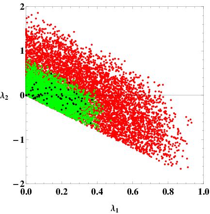
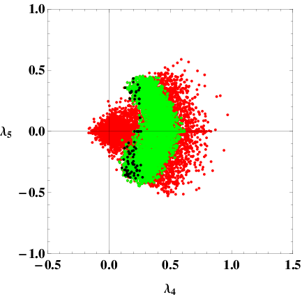
Figure 1 shows scatter plots in the (, ) plane (left) and the (, ) plane (right), which satisfy the vacuum stability and perturbativity conditions. The green dots in Fig. 1 correspond to the allowed parameter space for , in which the new quartic couplings (, ) should be sufficiently small to keep the perturbativity up to the Planck scale. The black dots satisfy . The lower bound of is because of , and the upper bounds of and come from the perturbativity condition. Since the third terms of the last four inequalities in Eq. (48) are negligible for a sufficiently large , the vacuum stability requires . Note that, when both and are small, the vacuum can become stable only by a sufficiently large , which will be explained in detail below. The allowed parameter space shown in Fig. 1 is much smaller than that in Ref. [13], in which only the unitarity condition has been considered.
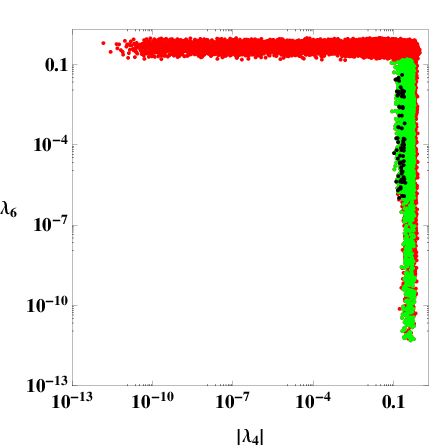
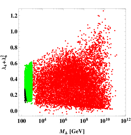
The left panel of Fig. 2 shows scatter plots in the (, ) plane. There is no allowed parameter space for and . Then we find for almost all values of , which is shown in the right panel of Fig. 2. If both and are sufficiently small, the Higgs mass correction would be smaller than the Higgs mass. However, the vacuum stability cannot be realized by such small parameters.
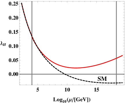
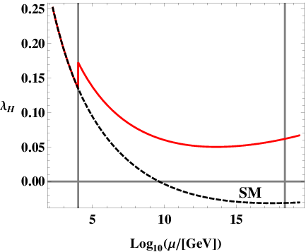
To stabilize the EW vacuum, there are two types of solutions. We show the running of for typical input parameters in Fig. 3. The left panel of Fig. 3 corresponds to the large positive contribution to a beta function of (), which is realized by a large and/or [see Eq. (70)]. The right panel of Fig. 3 corresponds to a discontinuous shift between and , which is realized by a large [see Eq. (47)]. When and are sufficiently small but is sufficiently large, the EW vacuum likely become stable, because also positively contributes to . In that case, however, the last two conditions in Eq. (48) cannot be satisfied. Thus, when the EW vacuum becomes stable, the Higgs mass correction usually becomes larger than the Higgs mass.
Figure 4 shows dependence of the Higgs mass correction, which is calculated by Eq. (51). From the right panel of Fig. 4, we find that the naturalness condition requires . Below this bound, the minimal type-II seesaw model can be testable by the LHC Run-II results [32] [also see Refs. [33]-[38] for the LHC phenomenology]. In the case of , from four-lepton signal at the 14 TeV LHC experiment with , we can potentially probe up to a mass for the normal (inverted) hierarchy of active neutrino masses. In the case of , with an integrated luminosity , the triplet scalars can be fully reconstructed at the 14 TeV LHC.


4.2 Predictions for the decay rate of ,
In the SM, the decay at the one-loop level is mediated by the virtual exchange of SM fermions (dominantly the top-quark) and the -boson. In the type-II seesaw model, there are additional contributions from the new charged Higgs bosons [10].22 2 There are also other contributions in extended type-II seesaw models, for example, in Refs. [41, 42]. The decay rates of is given by [39, 40]
| (56) | |||||
where is the fine-structure constant, is the Fermi coupling constant, for quarks (leptons), and is the electric charge of the fermion in the loop. In the same way, the decay rate of is given by
| (57) | |||||
where , , , (), and are the third isospin components of the fermion. In these equations, the first two terms in the squared amplitude are the SM fermion and -boson contributions, respectively, whereas the last two terms correspond to the and contributions. We consider only the top quark contribution for the SM fermion, because the other fermion contributions are negligible. The relevant loop functions are defined as
| (58) | |||||
where
| (59) |
with the functions and in the range , given by
| (60) |
The couplings of to the SM fermions and vector bosons relative to the SM Higgs couplings are given by
| (61) |
From Eqs. (43) and (45), we see in the limit , , , and hence the couplings of to the SM fermions and vector bosons are almost identical to the SM case. The couplings of to the charged Higgs bosons in Eq. (57) are given by
| (62) |
For the scalar trilinear couplings, we have
| (63) |
with the following definitions in terms of the parameters of the scalar potential (up to ) [10]:
| (64) | |||||
| (65) |
In the limit , Eqs. (64) and (65) can be written as
| (66) |
Thus, the signs of the couplings and , and hence, those of the and contributions to the amplitude in Eq. (56) are fixed by the scalar couplings and , respectively. The allowed parameter space by the vacuum stability and perturbativity conditions is shown in Fig. 1, and we can see that there is a small allowed region in .
| Amplitude | Fermions | -Boson | ||
|---|---|---|---|---|
In the SM, the -boson contributions to and dominate over those from the SM fermions, while the signs of the corresponding amplitudes and are opposite as shown in Table 1. The doubly charged scalar contribution usually dominates over the singly charged scalar contribution for both and amplitude because of the enhancement factor of four in Eqs. (56) and (57), which corresponds to the squared electric charge of . Since doubly charged scalar contributions are proportional to with the opposite sign to the -boson contribution, the both decay widths are enhanced for . For the same reason, the behavior reverses for .
In order to compare the model predictions for the signal strength with the SM value at the LHC, the partial decay widths of the processes can be expressed by
| (67) |
where with the mixing angle given by Eq. (45). Since in the limit , the SM-like Higgs production rate is almost the same as that in the SM. The branching ratios of all the Higgs decay channels are also the same as in the SM, except for and channels which may differ significantly, but their contribution to the total decay width remains negligible as in the SM. Hence, for our numerical purposes, we can simply assume defined in Eq. (67) to be the ratio of the partial decay widths for in the type-II seesaw model and in the SM.


Figure 5 shows (left) and (right) versus . The green and cyan dots correspond to and , respectively. The black dots satisfy . The red line in the left panel shows the lower bound on the current signal strength, which is obtained as by the combined analysis of ATLAS and CMS results [43]. Our result of needs more than 10 % precision to see the deviation, while the relative uncertainty on the is 0.1 for the combined Higgs analysis by the LHC experiment at 14 TeV with of integrated luminosity [44]. There is no useful experimental bound for at present [45]. The expected measured signal for is by the 14 TeV LHC experiment with [46].
In the case, both and are larger than unity with . The behavior reverses for : in the case, both and are smaller than unity with . Although can be enhanced by both and contributions for , there is no parameter space in region for [see the right panel in Fig. 1]. This result comes from the vacuum stability conditions, and we note that is not strongly enhanced compared to the literature; for example Ref. [47, 48].
In the case, contributions from to the decay rate vanish, while contributions from can be seen clearly. We can see from Table 1 that there is an anti-correlation between and for . To see this, we show the relation between and in Fig. 6. The gray dots correspond to with , and they lie in the and region. Since there is no allowed parameter space in with , the model cannot realize and at the same time.

5 Conclusion
We have studied the vacuum stability and perturbativity conditions in the minimal type-II seesaw model. Their conditions give characteristic constraints between model parameters as in Fig. 1. The vacuum stability can be realized by sufficiently large or , which leads to large Higgs mass corrections. To realize the naturalness condition (), we have found that heavy Higgs masses should be lower than . Below this bound, the minimal type-II seesaw model can be testable by the LHC Run-II results. Due to the triplet scalar field, branching ratios of the Higgs decay for are different from the standard model case. They strongly depend on the sign of , and there is an anti-correlation between and for with . From the recent ATLAS and CMS combined analysis for the signal strength of , we have also found that a large parameter region is to be excluded. Our result of needs more than 10 % precision to see the deviation, while the relative uncertainty on the is 0.1 for the combined Higgs analysis by the LHC experiment at 14 TeV with of integrated luminosity.
Acknowledgment
N. O. would like to thank the Particle Physics Theory Group of Shimane University for hospitality during his visit. This work is partially supported by Scientific Grants by the Ministry of Education, Culture, Sports, Science and Technology (Nos. 24540272, 26247038, and 15H01037) and the United States Department of Energy (DE-SC 0013680). The work of Y. Y. is supported by Research Fellowships of the Japan Society for the Promotion of Science for Young Scientists (Grants No. 262428).
Appendix
The beta functions in the minimal type-II seesaw model
The one-loop beta functions for the minimal type-II seesaw model are given by
| (68) | |||||
| (69) | |||||
| (70) | |||||
| (71) | |||||
| (72) | |||||
| (73) | |||||
| (74) | |||||
where we define and its beta function is given by
| (75) |
References
- [1] S. Weinberg, Phys. Rev. Lett. 43 (1979) 1566.
- [2]
P. Minkowski,
Phys. Lett. B 67, 421 (1977)
doi:10.1016/0370-2693(77)90435-X;
T. Yanagida, Conf. Proc. C 7902131, 95 (1979);
M. Gell-Mann, P. Ramond and R. Slansky, Conf. Proc. C 790927, 315 (1979) [arXiv:1306.4669 [hep-th]];
R. N. Mohapatra and G. Senjanovic, Phys. Rev. Lett. 44, 912 (1980) doi:10.1103/PhysRevLett.44.912;
J. Schechter and J. W. F. Valle, Phys. Rev. D 22, 2227 (1980); Phys. Rev. D 25 774 (1982). - [3] M. Magg and C. Wetterich, Phys. Lett. B 94, 61 (1980). doi:10.1016/0370-2693(80)90825-4
- [4] T. P. Cheng and L. F. Li, Phys. Rev. D 22, 2860 (1980). doi:10.1103/PhysRevD.22.2860
- [5] G. Lazarides, Q. Shafi and C. Wetterich, Nucl. Phys. B 181, 287 (1981). doi:10.1016/0550-3213(81)90354-0
- [6] R. N. Mohapatra and G. Senjanovic, Phys. Rev. D 23, 165 (1981). doi:10.1103/PhysRevD.23.165
- [7] R. Foot, H. Lew, X. G. He and G. C. Joshi, Z. Phys. C 44, 441 (1989). doi:10.1007/BF01415558
- [8] F. F. Deppisch, P. S. Bhupal Dev and A. Pilaftsis, New J. Phys. 17, no. 7, 075019 (2015) doi:10.1088/1367-2630/17/7/075019 [arXiv:1502.06541 [hep-ph]].
- [9] I. Gogoladze, N. Okada and Q. Shafi, Phys. Rev. D 78, 085005 (2008) doi:10.1103/PhysRevD.78.085005 [arXiv:0802.3257 [hep-ph]].
- [10] A. Arhrib, R. Benbrik, M. Chabab, G. Moultaka, M. C. Peyranere, L. Rahili and J. Ramadan, Phys. Rev. D 84, 095005 (2011) [arXiv:1105.1925 [hep-ph]].
- [11] W. Chao, M. Gonderinger and M. J. Ramsey-Musolf, Phys. Rev. D 86, 113017 (2012) doi:10.1103/PhysRevD.86.113017 [arXiv:1210.0491 [hep-ph]].
- [12] E. J. Chun, H. M. Lee and P. Sharma, JHEP 1211, 106 (2012) doi:10.1007/JHEP11(2012)106 [arXiv:1209.1303 [hep-ph]].
- [13] P. S. Bhupal Dev, D. K. Ghosh, N. Okada and I. Saha, JHEP 1303, 150 (2013) [JHEP 1305, 049 (2013)] [arXiv:1301.3453 [hep-ph]].
- [14] C. Bonilla, R. M. Fonseca and J. W. F. Valle, Phys. Rev. D 92, no. 7, 075028 (2015) doi:10.1103/PhysRevD.92.075028 [arXiv:1508.02323 [hep-ph]].
- [15] E. Accomando et al., hep-ph/0608079.
- [16] M. A. Schmidt, Phys. Rev. D 76, 073010 (2007) [Phys. Rev. D 85, 099903 (2012)] [arXiv:0705.3841 [hep-ph]].
- [17] J. Beringer et al. [Particle Data Group Collaboration], Phys. Rev. D 86, 010001 (2012).
- [18] Z. Maki, M. Nakagawa and S. Sakata, Prog. Theor. Phys. 28 (1962) 870;
- [19] B. Pontecorvo, Sov. Phys. JETP 26 (1968) 984 [Zh. Eksp. Teor. Fiz. 53 (1967) 1717].
- [20] K. A. Olive et al. [Particle Data Group Collaboration], Chin. Phys. C 38, 090001 (2014). doi:10.1088/1674-1137/38/9/090001
- [21] D. Buttazzo, G. Degrassi, P. P. Giardino, G. F. Giudice, F. Sala, A. Salvio and A. Strumia, JHEP 1312, 089 (2013) doi:10.1007/JHEP12(2013)089 [arXiv:1307.3536 [hep-ph]].
- [22] A. Abada, C. Biggio, F. Bonnet, M. B. Gavela and T. Hambye, JHEP 0712, 061 (2007) [arXiv:0707.4058 [hep-ph]].
- [23] M. Farina, D. Pappadopulo and A. Strumia, JHEP 1308, 022 (2013) doi:10.1007/JHEP08(2013)022 [arXiv:1303.7244 [hep-ph]].
- [24] M. Chabab, M. Capdequi-Peyranere and L. Rahili, arXiv:1512.07280 [hep-ph].
- [25] M. J. G. Veltman, Acta Phys. Polon. B 12, 437 (1981).
- [26] G. Aad et al. [ATLAS and CMS Collaborations], arXiv:1503.07589 [hep-ex].
- [27] [ATLAS and CDF and CMS and D0 Collaborations], arXiv:1403.4427 [hep-ex].
- [28] S. Bethke, Nucl. Phys. Proc. Suppl. 234, 229 (2013) [arXiv:1210.0325 [hep-ex]].
- [29] G. Aad et al. [ATLAS Collaboration], JHEP 1503, 041 (2015) [arXiv:1412.0237 [hep-ex]].
- [30] A. G. Akeroyd, M. Aoki and H. Sugiyama, Phys. Rev. D 79, 113010 (2009) [arXiv:0904.3640 [hep-ph]].
- [31] T. Fukuyama, H. Sugiyama and K. Tsumura, JHEP 1003, 044 (2010) [arXiv:0909.4943 [hep-ph]].
- [32] Z. L. Han, R. Ding and Y. Liao, Phys. Rev. D 91, 093006 (2015) doi:10.1103/PhysRevD.91.093006 [arXiv:1502.05242 [hep-ph]].
- [33] A. G. Akeroyd and M. Aoki, Phys. Rev. D 72, 035011 (2005) doi:10.1103/PhysRevD.72.035011 [hep-ph/0506176].
- [34] A. G. Akeroyd and H. Sugiyama, Phys. Rev. D 84, 035010 (2011) doi:10.1103/PhysRevD.84.035010 [arXiv:1105.2209 [hep-ph]].
- [35] M. Aoki, S. Kanemura and K. Yagyu, Phys. Rev. D 85, 055007 (2012) doi:10.1103/PhysRevD.85.055007 [arXiv:1110.4625 [hep-ph]].
- [36] A. G. Akeroyd, S. Moretti and H. Sugiyama, Phys. Rev. D 85, 055026 (2012) doi:10.1103/PhysRevD.85.055026 [arXiv:1201.5047 [hep-ph]].
- [37] E. J. Chun and P. Sharma, JHEP 1208, 162 (2012) doi:10.1007/JHEP08(2012)162 [arXiv:1206.6278 [hep-ph]].
- [38] E. J. Chun and P. Sharma, Phys. Lett. B 728, 256 (2014) doi:10.1016/j.physletb.2013.11.056 [arXiv:1309.6888 [hep-ph]].
- [39] C. S. Chen, C. Q. Geng, D. Huang and L. H. Tsai, Phys. Rev. D 87, 075019 (2013) [arXiv:1301.4694 [hep-ph]].
- [40] C. S. Chen, C. Q. Geng, D. Huang and L. H. Tsai, Phys. Lett. B 723, 156 (2013) [arXiv:1302.0502 [hep-ph]].
- [41] L. Wang and X. F. Han, Phys. Rev. D 87, no. 1, 015015 (2013) doi:10.1103/PhysRevD.87.015015 [arXiv:1209.0376 [hep-ph]].
- [42] E. J. Chun and P. Sharma, Phys. Lett. B 722, 86 (2013) doi:10.1016/j.physletb.2013.03.038 [arXiv:1301.1437 [hep-ph]].
- [43] The ATLAS and CMS Collaborations, ATLAS-CONF-2015-044.
- [44] ATLAS Collaboration, ATL-PHYS-PUB-2013-014.
- [45] G. Aad et al. [ATLAS Collaboration], Phys. Lett. B 732, 8 (2014) doi:10.1016/j.physletb.2014.03.015 [arXiv:1402.3051 [hep-ex]].
- [46] ATLAS Collaboration, ATL-PHYS-PUB-2014-006.
- [47] A. Arhrib, R. Benbrik, M. Chabab, G. Moultaka and L. Rahili, JHEP 1204, 136 (2012) [arXiv:1112.5453 [hep-ph]].
- [48] A. G. Akeroyd and S. Moretti, Phys. Rev. D 86, 035015 (2012) doi:10.1103/PhysRevD.86.035015 [arXiv:1206.0535 [hep-ph]].