跳到论文正文
W Papers独立论文阅读器 arXiv:1601.05038 论文正文 计算阅读时间 · 0%
引用这篇论文根据当前论文元数据生成,正式投稿前建议核对。


License: arXiv.org perpetual non-exclusive license
arXiv:1601.05038v1 [hep-ph] 19 Jan 2016

Renormalizable Model for Neutrino Mass, Dark Matter, Muon g−2g-2
and 750 GeV Diphoton Excess

Hiroshi Okada Affiliation: School of Physics, KIAS, Seoul 130-722, Korea Affiliation: Physics Division, National Center for Theoretical Sciences, Hsinchu, Taiwan 300    Kei Yagyu Affiliation: School of Physics and Astronomy, University of Southampton, Southampton, SO17 1BJ, United Kingdom
Abstract

We discuss a possibility to explain the 750 GeV diphoton excess observed at the LHC in a three-loop neutrino mass model which has a similar structure to the model by Krauss, Nasri and Trodden. Tiny neutrino masses are naturally generated by the loop effect of new particles with their couplings and masses to be of order 0.1-1 and TeV, respectively. The lightest right-handed neutrino, which runs in the three-loop diagram, can be a dark matter candidate. In addition, the deviation in the measured value of the muon anomalous magnetic moment from its prediction in the standard model can be compensated by one-loop diagrams with exotic multi-charged leptons and scalar bosons. For the diphoton event, an additional isospin singlet real scalar field plays the role to explain the excess by taking its mass of 750 GeV, where it is produced from the gluon fusion production via the mixing with the standard model like Higgs boson. We find that the cross section of the diphoton process can be obtained to be a few fb level by taking the masses of new charged particles to be about 375 GeV and related coupling constants to be order 1.

I Introduction

In December 2015, the both ATLAS and CMS groups have reported the existence of the excess at around 750 GeV in the diphoton distribution at the Large Hadron Collider (LHC) with the collision energy of 13 TeV. The local significance of this excess is about 3.6σ\sigma at ATLAS [1] with the integrated luminosity of 3.2 fb-1 and about 2.6σ\sigma at CMS [2] with the integrated luminosity of 2.6 fb-1. The detailed properties of the diphoton excess was summarized, e.g., in Ref. [3], where the best fit value of the width of the new resonance is about 45 GeV, and the estimated cross section of the diphoton signature is 10±310\pm 3 fb at ATLAS and 6±36\pm 3 fb at CMS. If this excess is confirmed by future data, it suggests the existence of a new particle which gives the direct evidence of a new physics beyond the standard model (SM).

The simplest way to explain this excess is to consider an extension of the SM by adding extra isospin scalar multiplets such as a singlet, a doublet and/or a triplet. However, it is difficult to get a sufficient cross section to explain the excess as mentioned in the above in such a simple extension of the SM. For example, if we consider the CP-conserving two Higgs doublet models (THDMs) [4, 5, 6, 7, 8], and take the masses of the additional CP-even HH and CP-odd AA Higgs bosons to be 750 GeV, then the cross section of p​p→H/A→γ​γpp\to H/A\to\gamma\gamma is typically three order smaller than the required value [4]. Therefore, we need to further introduce additional sources to get an enhancement of the production cross section and/or the branching fraction to the diphoton mode, e.g., by introducing multi-charged scalar particles [4, 6] and vector-like fermions [7]. In Refs. [8], the diphoton excess has been discussed in supersymmetric models.

In this paper, we discuss a scenario to naturally introduce multi-charged particles to get an enhancement of the branching fraction. Namely, we consider a radiative neutrino mass model in which multi-charged particles play a role not only to increase the branching fraction but also to explain the smallness of neutrino masses and the anomaly of the muon anomalous magnetic moment. A dark matter (DM) candidate can also successfully be involved as a part of the model. There are a few papers discussing the diphoton excess within radiative neutrino mass models [9]. In particular, we discuss a new three loop neutrino mass model11 1 Other variations of three loop neutrino mass models have also been proposed in Refs. [11, 12, 13, 14, 15, 16]. whose structure is similar to the model by Krauss, Nasri and Trodden in 2003 [10], because the three loop suppression factor 1/(16​π2)31/(16\pi^{2})^{3} is a suitable amount to reproduce the measured neutrino masses, i.e., 𝒪⁡(0.1){\cal O}(0.1) eV, by order 0.1-1 couplings and TeV scale masses of new particles. In our model, an additional isospin real singlet scalar field can explain the diphoton excess, where it is produced from the gluon fusion process through the mixing with the SM-like Higgs boson.

The plan of the paper is as follows. In Sec. II, we define our model, and give the Lagrangian for the lepton sector and the scalar potential. In Sec. III, we discuss the neutrino masses, the phenomenology of DM including the relic abundance and direct search experiments, and new contributions to the muon g−2g-2. The diphoton excess is discussed in Sec. IV. Our conclusion is summarized in Sec. V.

Lepton Fields Scalar Fields
LLiL_{L}^{i} eRie_{R}^{i} L5/2a=(L−−a,L−−−a)TL_{5/2}^{a}=(L^{--a},L^{---a})^{T} E−−aE^{--a} NRaN_{R}^{a} Φ\Phi κ+⁣+\kappa^{++} S+⁣+S^{++} Σ\Sigma
(S​U​(2)L,U​(1)Y)(SU(2)_{L},U(1)_{Y}) (𝟐,−1/2)(\bm{2},-1/2) (𝟏,−1)(\bm{1},-1) (𝟐,−5/2)(\bm{2},-5/2) (𝟏,−2)(\bm{1},-2) (𝟏,0)(\bm{1},0) (𝟐,1/2)(\bm{2},1/2) (𝟏,2)(\bm{1},2) (𝟏,2)(\bm{1},2) (𝟏,0)(\bm{1},0)
Z2Z_{2} ++ ++ −- −- −- ++ ++ −- ++
Table 1: Particle contents and charge assignments under S​U​(2)L×U​(1)Y×Z2SU(2)_{L}\times U(1)_{Y}\times Z_{2}. The superscripts ii and aa denote the flavor of the SM fermions and the exotic fermions with i=1​-​3i=1\text{-}3 and a=1​-​NEa=1\text{-}N_{E}, respectively.

II The Model

Our model is described by the SM gauge symmetry S​U​(2)L×U​(1)YSU(2)_{L}\times U(1)_{Y} and an additional discrete symmetry Z2Z_{2} which is assumed to be unbroken. This Z2Z_{2} symmetry is introduced to avoid tree level contributions to neutrino masses and to enclose the three-loop diagram as shown in Fig. 1. Because of the Z2Z_{2} symmetry, the stability of the lightest neutral Z2Z_{2} odd particle is guaranteed, and thus it can be a candidate of DM.

The particle contents are shown in Table 1, where LLiL_{L}^{i} and eRie_{R}^{i} are the SM left-handed lepton doublets and lepton singlets with the flavor of ii (i=i=1-3). In addition, we add the NEN_{E} flavor of the vector like lepton doublets (singlets) L5/2a=(L−−a,L−−−a)TL_{5/2}^{a}=(L^{--a},L^{---a})^{T} (E−−aE^{--a}) with the hypercharge Y=−5/2Y=-5/2 (−2-2) and the right-handed neutrinos NRaN_{R}^{a} (a=1a=1-NEN_{E}). The scalar sector is composed of one isospin doublet field Φ\Phi with Y=1/2Y=1/2 and two complex (one real) isospin singlet scalar fields κ+⁣+\kappa^{++} and S+⁣+S^{++} with Y=2Y=2 (Σ\Sigma with Y=0Y=0). The doublet and the real singlet scalar fields are parameterized by

Φ=(G+v+ϕ0+i​G02),Σ=σ0+vσ,\displaystyle\Phi=\begin{pmatrix}G^{+}\\ \frac{v+\phi^{0}+iG^{0}}{\sqrt{2}}\end{pmatrix},\quad\Sigma=\sigma^{0}+v_{\sigma}, (1)

where vv and vσv_{\sigma} are the vacuum expectation values (VEVs) of doublet and singlet scalar fields, respectively, and G+G^{+} (G0)(G^{0}) denotes the Nambu-Goldstone boson which is absorbed into the longitudinal component of the WW (Z)(Z) boson. The Fermi constant GFG_{F} is given by the usual relation, i.e., GF=1/(2​v2)G_{F}=1/(\sqrt{2}v^{2}) with v≃246v\simeq 246 GeV. The singlet VEV vσv_{\sigma} does not contribute to the electroweak symmetry breaking. We note that the shift vσ→vσ′v_{\sigma}\to v_{\sigma}^{\prime} does not change any physical quantities, because its impact can be absorbed by the redefinition of the parameters in the Lagrangian. We thus take vσ=0v_{\sigma}=0 in the following discussion to make some expressions to be a simple form.

The most general Lagrangian for the lepton fields is given by

−ℒlep\displaystyle-\mathcal{L}_{\text{lep}} =12MNaNRa​c¯NRa+MLa(L5/2a)L¯(L5/2a)R+MEaE−−aL¯ER−−a+h.c.\displaystyle=\frac{1}{2}M_{N}^{a}\overline{N^{ac}_{R}}N_{R}^{a}+M_{L}^{a}\overline{(L_{5/2}^{a})_{L}}(L_{5/2}^{a})_{R}+M_{E}^{a}\overline{E^{--a}_{L}}E^{--a}_{R}+{\rm h.c.}
+ySMiLLi¯ΦeRi+y1a​b(L5/2a)L¯Φ~ER−−b+y2a​b(L5/2a)R¯Φ~EL−−b+h.c.\displaystyle+y_{\text{SM}}^{i}\,\overline{L_{L}^{i}}\Phi\,e_{R}^{i}+y_{1}^{ab}\,\overline{(L_{5/2}^{a})_{L}}\tilde{\Phi}\,E_{R}^{--b}+y_{2}^{ab}\,\overline{(L_{5/2}^{a})_{R}}\tilde{\Phi}\,E_{L}^{--b}+{\rm h.c.}
+gLa​b(L5/2a)L¯(L5/2a)RΣ+gEa​b(E−−a)L¯ER−−bΣ+gNa​bNRa​c¯NRbΣ+h.c.\displaystyle+g_{L}^{ab}\,\overline{(L_{5/2}^{a})_{L}}(L_{5/2}^{a})_{R}\,\Sigma+g_{E}^{ab}\,\overline{(E^{--a})_{L}}\,E_{R}^{--b}\,\Sigma+g_{N}^{ab}\overline{N_{R}^{ac}}\,N_{R}^{b}\,\Sigma+{\rm h.c.}
+h0i​jeRi​c¯eRjκ+⁣++h1a​bNRa¯EL−−bκ+⁣++h2a​bNRa​c¯ER−−bκ+⁣++fi​aLLi¯(L5/2a)RS+⁣++h.c.,\displaystyle+h_{0}^{ij}\,\overline{e_{R}^{ic}}\,e_{R}^{j}\,\kappa^{++}+h_{1}^{ab}\,\overline{N_{R}^{a}}E^{--b}_{L}\,\kappa^{++}+h_{2}^{ab}\,\overline{N_{R}^{ac}}E^{--b}_{R}\kappa^{++}+f^{ia}\,\overline{L^{i}_{L}}(L_{5/2}^{a})_{R}\,S^{++}+{\rm h.c.}, (2)

where Φ~=i​σ2​Φ∗\tilde{\Phi}=i\sigma_{2}\Phi^{*}. We can take the diagonal form of the invariant masses MNaM_{N}^{a}, MLaM_{L}^{a} and MEaM_{E}^{a} for the vector like leptons L5/2aL_{5/2}^{a}, EaE^{a} and right-handed neutrinos NRaN_{R}^{a}, respectively, without loss of generality. The SM leptons LLL_{L} and eRe_{R} are taken to be the mass eigenstates, so that the Yukawa coupling ySMiy_{\text{SM}}^{i} is given by the diagonal form. For simplicity, we assume that all the above parameters are real.

The most general Higgs potential is given by

V⁡(Φ,κ+⁣+,S+⁣+,Σ)=VHSM​(Φ,Σ)+μκ2​(κ+⁣+​κ−⁣−)+μS2​(S+⁣+​S−⁣−)\displaystyle V(\Phi,\kappa^{++},S^{++},\Sigma)=V_{\text{HSM}}(\Phi,\Sigma)+\mu_{\kappa}^{2}(\kappa^{++}\kappa^{--})+\mu_{S}^{2}(S^{++}S^{--})
+AΣ​κ​Σ​(κ+⁣+​κ−⁣−)+AΣ​S​Σ​(S+⁣+​S−⁣−)\displaystyle+A_{\Sigma\kappa}\,\Sigma\,(\kappa^{++}\kappa^{--})+A_{\Sigma S}\Sigma\,(S^{++}S^{--})
+λΦ​κ​(Φ†​Φ)​(κ+⁣+​κ−⁣−)+λΦ​S​(Φ†​Φ)​(S+⁣+​S−⁣−)+λΣ​κ​Σ2​(κ+⁣+​κ−⁣−)+λΣ​S​Σ2​(S+⁣+​S−⁣−)\displaystyle+\lambda_{\Phi\kappa}(\Phi^{\dagger}\Phi)(\kappa^{++}\kappa^{--})+\lambda_{\Phi S}(\Phi^{\dagger}\Phi)(S^{++}S^{--})+\lambda_{\Sigma\kappa}\Sigma^{2}(\kappa^{++}\kappa^{--})+\lambda_{\Sigma S}\Sigma^{2}(S^{++}S^{--})
+λκ​(κ+⁣+​κ−⁣−)2+λS​(S+⁣+​S−⁣−)2+λκ​S​(κ+⁣+​κ−⁣−)​(S+⁣+​S−⁣−)\displaystyle+\lambda_{\kappa}(\kappa^{++}\kappa^{--})^{2}+\lambda_{S}(S^{++}S^{--})^{2}+\lambda_{\kappa S}(\kappa^{++}\kappa^{--})(S^{++}S^{--})
+[λ0​(κ+⁣+​S−⁣−)​(κ+⁣+​S−⁣−)+h.c.],\displaystyle+[\lambda_{0}(\kappa^{++}S^{--})(\kappa^{++}S^{--})+\text{h.c.}], (3)

where the complex phase of the λ0\lambda_{0} parameter can be absorbed by rephasing the scalar fields. The squared masses of the doubly-charged scalar bosons S±⁣±S^{\pm\pm} and κ±⁣±\kappa^{\pm\pm} are given by

mκ±⁣±2=μκ2+v22​λΦ​κ,mS±⁣±2=μS2+v22​λΦ​S.\displaystyle m_{\kappa^{\pm\pm}}^{2}=\mu_{\kappa}^{2}+\frac{v^{2}}{2}\lambda_{\Phi\kappa},\quad m_{S^{\pm\pm}}^{2}=\mu_{S}^{2}+\frac{v^{2}}{2}\lambda_{\Phi S}. (4)

In Eq. (3), the VHSMV_{\text{HSM}} part is given as the same form as in the Higgs singlet model (HSM) involving Φ\Phi and Σ\Sigma as

VHSM​(Φ,Σ)=\displaystyle V_{\text{HSM}}(\Phi,\Sigma)= μΦ2​(Φ†​Φ)+λ​(Φ†​Φ)2+AΦ​Σ​(Φ†​Φ)​Σ+λΦ​Σ​(Φ†​Φ)​Σ2\displaystyle\mu_{\Phi}^{2}(\Phi^{\dagger}\Phi)+\lambda(\Phi^{\dagger}\Phi)^{2}+A_{\Phi\Sigma}(\Phi^{\dagger}\Phi)\Sigma+\lambda_{\Phi\Sigma}(\Phi^{\dagger}\Phi)\Sigma^{2}
+tΣ​Σ+μΣ2​Σ2+AΣ​Σ3+λΣ​Σ4.\displaystyle+t_{\Sigma}\Sigma+\mu^{2}_{\Sigma}\Sigma^{2}+A_{\Sigma}\Sigma^{3}+\lambda_{\Sigma}\Sigma^{4}. (5)

Two CP-even scalar states ϕ0\phi^{0} from the doublet and s0s^{0} from the singlet are mixed with each other via the mixing angle α\alpha defined as

(σ0ϕ0)=(cos⁡α−sin⁡αsin⁡αcos⁡α)​(Hh).\displaystyle\begin{pmatrix}\sigma^{0}\\ \phi^{0}\end{pmatrix}=\begin{pmatrix}\cos\alpha&-\sin\alpha\\ \sin\alpha&\cos\alpha\end{pmatrix}\begin{pmatrix}H\\ h\end{pmatrix}. (6)

We define hh as the SM-like Higgs boson with the mass of about 125 GeV which is identified as the discovered Higgs boson at the LHC. The detailed expressions for the masses of the CP-even Higgs bosons and the mixing angle α\alpha in terms of the potential parameters are given, e.g., in Ref. [17].

The masses of the exotic charged leptons are obtained from two sources, i.e., the invariant mass terms MEM_{E} and MLM_{L} and the Yukawa interaction terms y1y_{1} and y2y_{2}. The mass of the triply-charged leptons L−−−aL^{---a} is simply given by MLaM_{L}^{a}. For the doubly-charged leptons, there is a mixing between L−−aL^{--a} and E−−aE^{--a} through the y1y_{1} and y2y_{2} terms. The mass matrix is given assuming y1a​b=y2a​b=yEa=diag​(yE1,…,yENE)y_{1}^{ab}=y_{2}^{ab}=y_{E}^{a}=\text{diag}(y_{E}^{1},\dots,y_{E}^{N_{E}}) by

ℒmass\displaystyle{\cal L}_{\text{mass}} =−(E−−a¯,L−−a¯)​(MEaMDaMDaMLa)​(E−−aL−−a)=−(E1−−a¯,E2−−a¯)​(ME1a00ME2a)​(E1−−aE2−−a),\displaystyle=-(\overline{E^{--a}},\overline{L^{--a}})\begin{pmatrix}M_{E}^{a}&M_{D}^{a}\\ M_{D}^{a}&M_{L}^{a}\end{pmatrix}\begin{pmatrix}E^{--a}\\ L^{--a}\end{pmatrix}=-(\overline{E_{1}^{--a}},\overline{E_{2}^{--a}})\begin{pmatrix}M_{E_{1}}^{a}&0\\ 0&M_{E_{2}}^{a}\end{pmatrix}\begin{pmatrix}E_{1}^{--a}\\ E_{2}^{--a}\end{pmatrix}, (7)

where MDa=v2​yEaM_{D}^{a}=\frac{v}{\sqrt{2}}y_{E}^{a}. The mass eigenstates E1aE_{1}^{a} and E2aE_{2}^{a} are defined by the orthogonal transformation:

(E−−aL−−a)=(cos⁡θa−sin⁡θasin⁡θacos⁡θa)​(E1−−aE2−−a).\displaystyle\begin{pmatrix}E^{--a}\\ L^{--a}\end{pmatrix}=\begin{pmatrix}\cos\theta_{a}&-\sin\theta_{a}\\ \sin\theta_{a}&\cos\theta_{a}\end{pmatrix}\begin{pmatrix}E_{1}^{--a}\\ E_{2}^{--a}\end{pmatrix}. (8)

The mass eigenvalues (ME1a≤ME2aM_{E_{1}}^{a}\leq M_{E_{2}}^{a}) and the mixing angles θa\theta_{a} are given by

ME1,2a\displaystyle M_{E_{1,2}}^{a} =12​(MEa+MLa∓(MEa−MLa)2+4​(MDa)2),\displaystyle=\frac{1}{2}\left(M_{E}^{a}+M_{L}^{a}\mp\sqrt{(M_{E}^{a}-M_{L}^{a})^{2}+4(M_{D}^{a})^{2}}\right), (9)
tan⁡2​θa\displaystyle\tan 2\theta_{a} =2​MDaMEa−MLa.\displaystyle=\frac{2M_{D}^{a}}{M_{E}^{a}-M_{L}^{a}}. (10)
Refer to caption
Figure 1: Three-loop neutrino mass diagram. Particles indicated by the red color are Z2Z_{2} odd, where Eα−−aE_{\alpha}^{--a} and Eβ−−cE_{\beta}^{--c} denote the mass eigenstates for the doubly-charged exotic leptons. The subscripts α\alpha and β\beta (run over 1 and 2) label two mass eigenstates for each flavor.

III Neutrino Mass, Dark Matter, Muon g−2g-2

III.1 Neutrino Mass

The leading contribution to the active neutrino mass matrix mνm_{\nu} is given at three-loop level as shown in Fig. 1. One- and two-loop diagrams which have been systematically classified in Refs. [18, 19] are absent in our setup. The three-loop diagram is computed as follows

(mν)i​j=λ0(16​π2)3​Mmax2\displaystyle(m_{\nu})_{ij}=\frac{\lambda_{0}}{(16\pi^{2})^{3}M^{2}_{\rm max}}
×∑a,b,c=13∑α,β=12cα​βfia∗sin2θaMEαah1b​aMNbh1b​csin2θcMEβcfjc∗F(rEαa,rNb,rEβc,rS±⁣±,rκ±⁣±),\displaystyle\times\sum_{a,b,c=1}^{3}\sum_{\alpha,\beta=1}^{2}c_{\alpha\beta}f^{ia*}\,\sin 2\theta_{a}M^{a}_{E_{\alpha}}h^{ba}_{1}M_{N}^{b}h_{1}^{bc}\,\sin 2\theta_{c}\,M^{c}_{E_{\beta}}f^{jc*}F(r_{E_{\alpha}^{a}},r_{N^{b}},r_{E_{\beta}^{c}},r_{S^{\pm\pm}},r_{\kappa^{\pm\pm}}), (11)

where we define rX≡(mX/Mmax)2r_{X}\equiv(m_{X}/M_{\rm max})^{2} with Mmax=Max⁡(MEαa,MEβc,MNb,mS±⁣±,mκ±⁣±)M_{\rm max}={\rm Max}(M_{E_{\alpha}^{a}},M_{E_{\beta}^{c}},M_{N^{b}},m_{S^{\pm\pm}},m_{\kappa^{\pm\pm}}) and mXm_{X} is the mass of a particle XX, and cα​β=1​(−1)c_{\alpha\beta}=1\,(-1) for α=β⁡(α≠β)\alpha=\beta\,(\alpha\neq\beta). The three loop function FF is given by

F⁡(rEαa,rNb,rEβc,rS±⁣±,rκ±⁣±)=∫01d​x1​d​y1​d​z1​δ​(1−x1−y1−z1)​1z12−z1\displaystyle F(r_{E_{\alpha}^{a}},r_{N^{b}},r_{E_{\beta}^{c}},r_{S^{\pm\pm}},r_{\kappa^{\pm\pm}})=\int_{0}^{1}dx_{1}dy_{1}dz_{1}\delta(1-x_{1}-y_{1}-z_{1})\frac{1}{z_{1}^{2}-z_{1}}
×∫01d​x2​d​y2​d​z2​δ​(1−x2−y2−z2)​1z22−z2​∫01d​x3​d​y3​d​z3​δ​(1−x3−y3−z3)​1Δ3,\displaystyle\times\int_{0}^{1}dx_{2}dy_{2}dz_{2}\delta(1-x_{2}-y_{2}-z_{2})\frac{1}{z_{2}^{2}-z_{2}}\,\int_{0}^{1}dx_{3}dy_{3}dz_{3}\delta(1-x_{3}-y_{3}-z_{3})\frac{1}{\Delta_{3}}, (12)

where

Δ3=x3​rEαa+y3​rS±⁣±+z3​Δ2,\displaystyle\Delta_{3}=x_{3}r_{E_{\alpha}^{a}}+y_{3}r_{S^{\pm\pm}}+z_{3}\Delta_{2}, (13)
with​Δ2=−x2​rNb+y2​Δ1+z2​rκ±⁣±z22−z2,and​Δ1=−x​rEβc+y​rS±⁣±+z​rκ±⁣±z12−z1.\displaystyle\text{with}~~\Delta_{2}=-\frac{x_{2}r_{N^{b}}+y_{2}\Delta_{1}+z_{2}r_{\kappa^{\pm\pm}}}{z_{2}^{2}-z_{2}},~~\text{and}~~\Delta_{1}=-\frac{xr_{E_{\beta}^{c}}+yr_{S^{\pm\pm}}+zr_{\kappa^{\pm\pm}}}{z_{1}^{2}-z_{1}}. (14)

The interval of the integrals in Eq. (12) for all the variables is from 0 to 1, i.e., ∫01d​x​𝑑y​𝑑z=∫01d​x​∫01d​y​∫01𝑑z\int_{0}^{1}dxdydz=\int_{0}^{1}dx\int_{0}^{1}dy\int_{0}^{1}dz. Typical values of FF with ri=(0.1,1)r_{i}=(0.1,1) are 𝒪⁡(1){\cal O}(1). Let us estimate magnitudes of couplings and masses to reproduce the magnitude of neutrino masses, i.e., the order of 0.1 eV. For simplicity, when we take Mmax=MEαa∼MEβc∼MNbM_{\text{max}}=M_{E_{\alpha}^{a}}\sim M_{E_{\beta}^{c}}\sim M_{N^{b}}, the neutrino masses are approximately expressed as

(mν)i​j\displaystyle(m_{\nu})_{ij} ∼Mmax(16​π2)3×Ki​j∼(0.1​eV)×106×(Mmaxv)×Ki​j,\displaystyle\sim\frac{M_{\rm max}}{(16\pi^{2})^{3}}\times K_{ij}\sim(0.1~\text{eV})\times 10^{6}\times\left(\frac{M_{\text{max}}}{v}\right)\times K_{ij}, (15)
withKi​j=∑a,b,c=13fia∗hb​a1h1b​cfjc∗,\displaystyle\text{with}~~K_{ij}=\sum_{a,b,c=1}^{3}f^{ia*}\,h^{ba}_{1}h_{1}^{bc}f^{jc*}, (16)

where we assume λ0×F=𝒪⁡(1)\lambda_{0}\times F={\cal O}(1). Therefore, in the range of Mmax=v​-​10​vM_{\text{max}}=v\text{-}10\,v, the magnitude of the mixing factor Ki​jK_{ij} is required to be 𝒪⁡(10−7​-​10−6){\cal O}(10^{-7}\text{-}10^{-6}).

III.2 Dark Matter

Assuming that the right-handed neutrino NR1N_{R}^{1} is the lightest among all the Z2Z_{2} odd particles, NR1N_{R}^{1} looses its decay modes into any other lighter particles, and then it becomes stable. We thus can regard NR1N_{R}^{1} as the DM candidate in our model. The annihilation cross section is then calculated as

σ​vrel≈∫0πd​θ​sin⁡θ​∫02​πd​ϕ​1128​π2​s​|ℳ¯​(𝒩ℛ∞​𝒩ℛ∞→𝒜ℬ)|∈​∞−△⇕∈fin∫,\displaystyle\sigma v_{\rm rel}\approx\int_{0}^{\pi}d\theta\sin\theta\int_{0}^{2\pi}d\phi\frac{1}{128\pi^{2}s}|\overline{\cal M}(N_{R}^{1}N_{R}^{1}\to AB)|^{2}\sqrt{1-\frac{4m^{2}_{\text{fin}}}{s}}, (17)

where mfinm_{\text{fin}} is the mass of the final state particle. In the above expression, |ℳ¯​(𝒩ℛ∞​𝒩ℛ∞→𝒜ℬ)|∈|\overline{\cal M}(N_{R}^{1}N_{R}^{1}\to AB)|^{2} is the squared amplitude for the following two body to two body processes:

|ℳ¯(𝒩ℛ∞𝒩ℛ∞→𝒜ℬ)|∈=|ℳ¯(𝒩ℛ∞𝒩ℛ∞→κ+⁣+κ−⁣−)|∈+|ℳ¯(𝒩ℛ∞𝒩ℛ∞→{{¯)|∈+|ℳ¯(𝒩ℛ∞𝒩ℛ∞→𝒵𝒵)|∈\displaystyle|\overline{\cal M}(N_{R}^{1}N_{R}^{1}\to AB)|^{2}=|\overline{\cal M}(N_{R}^{1}N_{R}^{1}\to\kappa^{++}\kappa^{--})|^{2}+|\overline{\mathcal{M}}(N_{R}^{1}N_{R}^{1}\to f\bar{f})|^{2}+|\overline{\mathcal{M}}(N_{R}^{1}N_{R}^{1}\to ZZ)|^{2}
+|ℳ¯​(NR1​NR1→W+​W−)|2+|ℳ¯​(NR1​NR1→h​h)|2+|ℳ¯​(NR1​NR1→H​H)|2,\displaystyle+|\overline{\mathcal{M}}(N_{R}^{1}N_{R}^{1}\to W^{+}W^{-})|^{2}+|\overline{\mathcal{M}}(N_{R}^{1}N_{R}^{1}\to hh)|^{2}+|\overline{\mathcal{M}}(N_{R}^{1}N_{R}^{1}\to HH)|^{2}, (18)

The first annihilation process NR1​NR1→κ+⁣+​κ−⁣−N_{R}^{1}N_{R}^{1}\to\kappa^{++}\kappa^{--} happens through the tt- and uu-channels of the EαaE_{\alpha}^{a} mediation, where the doubly-charged scalar bosons κ±⁣±\kappa^{\pm\pm} decays into the same sign dilepton via the Yukawa coupling h0h_{0}. The squared amplitude of the NR1​NR1→κ+⁣+​κ−⁣−N_{R}^{1}N_{R}^{1}\to\kappa^{++}\kappa^{--} process is given by

|ℳ¯(𝒩ℛ∞𝒩ℛ∞→κ+⁣+κ−⁣−)|∈=∑⊣=∞𝒩ℰ|⟨∞⊣|∈⊔∇[(√/∈−ℳ𝒩∞)𝒳⊣(√/∞+ℳ𝒩∞)𝒳⊣†],\displaystyle|\overline{\cal M}(N_{R}^{1}N_{R}^{1}\to\kappa^{++}\kappa^{--})|^{2}=\sum_{a=1}^{N_{E}}|h^{1a}|^{2}{\rm tr}\left[(p\hskip-5.97508pt/\penalty_{2}-M_{N}^{1})X_{a}(p\hskip-5.97508pt/\penalty_{1}+M_{N}^{1})X_{a}^{\dagger}\right], (19)
Xa=cos2θa[−p/1+k/1+MaE1t−(ME1a)2+−p/1+k/2+MaE1u−(ME1a)2]+(cosθa→sinθa,ME1a→ME2a),\displaystyle X_{a}=\cos^{2}\theta_{a}\left[\frac{-p\hskip-5.97508pt/\penalty_{1}+k\hskip-5.97508pt/\penalty_{1}+M^{a}_{E_{1}}}{t-(M^{a}_{E_{1}})^{2}}+\frac{-p\hskip-5.97508pt/\penalty_{1}+k\hskip-5.97508pt/\penalty_{2}+M^{a}_{E_{1}}}{u-(M^{a}_{E_{1}})^{2}}\right]+(\cos\theta_{a}\to\sin\theta_{a},\,M^{a}_{E_{1}}\to M^{a}_{E_{2}}), (20)

where ss, tt and uu are the Mandelstam variables, NcfN_{c}^{f} is the color factor, and (p1,p2)(p_{1},p_{2}) and (k1,k2)(k_{1},k_{2}) are the initial and the final state momenta, respectively. In this expression, we take ha​b≡h1a​b=h2a​bh^{ab}\equiv h_{1}^{ab}=h_{2}^{ab} for simplicity. The other cross sections are given through the mixing of α\alpha via the ss-channel mediation of hh and HH by

|ℳ¯​(NR1​NR1→f​f¯)|2\displaystyle|\overline{\mathcal{M}}(N_{R}^{1}N_{R}^{1}\to f\bar{f})|^{2} =16​Ncf​(gN11​mf​sα​cαv)2​|1s−mh2+i​mh​Γh−1s−mH2+i​mH​ΓH|2\displaystyle=16{N_{c}^{f}}\left(\frac{g^{11}_{N}m_{f}s_{\alpha}c_{\alpha}}{v}\right)^{2}\left|\frac{1}{s-m_{h}^{2}+im_{h}\Gamma_{h}}-\frac{1}{s-m_{H}^{2}+im_{H}\Gamma_{H}}\right|^{2}
×[(p1⋅p2)−(MN1)2]​[(k1⋅k2)−mf2],\displaystyle\quad\times\left[(p_{1}\cdot p_{2})-(M_{N}^{1})^{2}\right]\left[(k_{1}\cdot k_{2})-m_{f}^{2}\right], (21)
|ℳ¯​(NR1​NR1→Z​Z)|2\displaystyle|\overline{\mathcal{M}}(N_{R}^{1}N_{R}^{1}\to ZZ)|^{2} =8​(gN11​mZ2​sα​cαv)2​|1s−mh2+i​mh​Γh−1s−mH2+i​mH​ΓH|2\displaystyle=8\left(\frac{g^{11}_{N}m_{Z}^{2}s_{\alpha}c_{\alpha}}{v}\right)^{2}\left|\frac{1}{s-m_{h}^{2}+im_{h}\Gamma_{h}}-\frac{1}{s-m_{H}^{2}+im_{H}\Gamma_{H}}\right|^{2}
×[(p1⋅p2)−(MN1)2]​[2+(k1⋅k2)2mZ4],\displaystyle\quad\times\left[(p_{1}\cdot p_{2})-(M_{N}^{1})^{2}\right]\left[2+\frac{(k_{1}\cdot k_{2})^{2}}{m_{Z}^{4}}\right], (22)
|ℳ¯​(NR1​NR1→W+​W−)|2\displaystyle|\overline{\mathcal{M}}(N_{R}^{1}N_{R}^{1}\to W^{+}W^{-})|^{2} =16​(gN11​mW2​sα​cαv)2​|1s−mh2+i​mh​Γh−1s−mH2+i​mH​ΓH|2\displaystyle=16\left(\frac{g^{11}_{N}m_{W}^{2}s_{\alpha}c_{\alpha}}{v}\right)^{2}\left|\frac{1}{s-m_{h}^{2}+im_{h}\Gamma_{h}}-\frac{1}{s-m_{H}^{2}+im_{H}\Gamma_{H}}\right|^{2}
×[(p1⋅p2)−(MN1)2]​[2+(k1⋅k2)2mW4],\displaystyle\quad\times\left[(p_{1}\cdot p_{2})-(M_{N}^{1})^{2}\right]\left[2+\frac{(k_{1}\cdot k_{2})^{2}}{m_{W}^{4}}\right], (23)
|ℳ¯​(NR1​NR1→h​h)|2\displaystyle|\overline{\mathcal{M}}(N_{R}^{1}N_{R}^{1}\to hh)|^{2} =2​(gN11)2​|sα​λh​h​hs−mh2+i​mh​Γh−cα​λH​h​hs−mH2+i​mH​ΓH|2\displaystyle=2\left({g^{11}_{N}}{}\right)^{2}\left|\frac{s_{\alpha}\lambda_{hhh}}{s-m_{h}^{2}+im_{h}\Gamma_{h}}-\frac{c_{\alpha}\lambda_{Hhh}}{s-m_{H}^{2}+im_{H}\Gamma_{H}}\right|^{2}
×[(p1⋅p2)−(MN1)2],\displaystyle\quad\times\left[(p_{1}\cdot p_{2})-(M_{N}^{1})^{2}\right], (24)
|ℳ¯​(NR1​NR1→H​H)|2\displaystyle|\overline{\mathcal{M}}(N_{R}^{1}N_{R}^{1}\to HH)|^{2} =2​(gN11)2​|sα​λh​H​Hs−mh2+i​mh​Γh−cα​λH​H​Hs−mH2+i​mH​ΓH|2\displaystyle=2\left({g^{11}_{N}}{}\right)^{2}\left|\frac{s_{\alpha}\lambda_{hHH}}{s-m_{h}^{2}+im_{h}\Gamma_{h}}-\frac{c_{\alpha}\lambda_{HHH}}{s-m_{H}^{2}+im_{H}\Gamma_{H}}\right|^{2}
×[(p1⋅p2)−(MN1)2],\displaystyle\quad\times\left[(p_{1}\cdot p_{2})-(M_{N}^{1})^{2}\right], (25)

where we use the short-hand notations of cα≡cos⁡αc_{\alpha}\equiv\cos{\alpha} and sα≡sin⁡αs_{\alpha}\equiv\sin{\alpha}. The dimensionful λφi​φj​φk\lambda_{\varphi_{i}\varphi_{j}\varphi_{k}} couplings (φi,j,k=h\varphi_{i,j,k}=h or HH) are defined by the coefficient of the scalar trilinear vertex in the potential. We note that the ss-wave contribution to σ​vrel\sigma v_{\rm rel} vanishes due to the Majorana property of the DM. To reproduce the observed relic density, the cross section given in Eq. (17) should be inside the following region

σ​vrel=(1.78​-​1.97)×10−9​GeV−2,\displaystyle\sigma{v_{\rm rel}}=(1.78\text{-}1.97)\times 10^{-9}\ {\rm GeV^{-2}}, (26)

at the 2​σ2\sigma level [20].

We also consider the spin independent scattering cross section with a neutron that is induced via the tree level diagram with the Higgs boson hh and HH exchange. The formula is given by

σSIn=C2π​(mn2​MN1mn+MN1)2​(gN11​cα​sαv)2​(−1mh2+1mH2)2,\displaystyle\sigma_{\text{SI}}^{n}=\frac{C^{2}}{\pi}\left(\frac{m_{n}^{2}M_{N}^{1}}{m_{n}+M_{N}^{1}}\right)^{2}\left(\frac{g^{11}_{N}c_{\alpha}s_{\alpha}}{v}\right)^{2}\left(-\frac{1}{m_{h}^{2}}+\frac{1}{m_{H}^{2}}\right)^{2}, (27)

where the neutron mass is mn≃0.939m_{n}\simeq 0.939 GeV and the factor C≃0.2872C\simeq 0.287^{2} is determined by the lattice simulation. The latest upper bound is reported by the LUX experiment that suggests σSIn≲10−45\sigma_{\text{SI}}^{n}\lesssim 10^{-45} cm for the DM mass of about 100 GeV with the 90 % C.L. [21].

III.3 Muon g−2g-2

The muon anomalous magnetic moment (muon g−2g-2) is one of the most promising low energy observables which suggest the existence of new physics beyond the SM. This is because there is the more than 3σ\sigma deviation in the SM prediction from the experimental value measured at Brookhaven National Laboratory. The difference Δ​aμ≡aμexp−aμSM\Delta a_{\mu}\equiv a^{\rm exp}_{\mu}-a^{\rm SM}_{\mu} has been calculated in Ref. [22] as

Δ​aμ=(29.0±9.0)×10−10.\displaystyle\Delta a_{\mu}=(29.0\pm 9.0)\times 10^{-10}. (28)

This shows the 3.2​σ3.2\sigma deviation in the SM prediction.

In our model, two diagrams contribute to Δ​aμ\Delta a_{\mu}, where L−−−aL^{---a}-S−−aS^{--a} and ℓ−\ell^{-}-κ−−a\kappa^{--a} with ℓ−\ell^{-} being the SM lepton are running in the loop. These contributions are calculated by

Δaμ≃mμ216​π2{\displaystyle\Delta a_{\mu}\simeq\frac{m_{\mu}^{2}}{16\pi^{2}}\Bigg\{ ∑a=1NE|fμ​a|2[3MLa​2G(mS±⁣±2MLa​2)+2mS±⁣±2G(MLa​2mS±⁣±2)]−∑i=13|h¯0μ​i|223​mκ±⁣±2}\displaystyle\sum_{a=1}^{N_{E}}|f^{\mu a}|^{2}\left[\frac{3}{M_{L}^{a2}}G\left(\frac{m_{S^{\pm\pm}}^{2}}{M_{L}^{a2}}\right)+\frac{2}{m_{S^{\pm\pm}}^{2}}G\left(\frac{M_{L}^{a2}}{m_{S^{\pm\pm}}^{2}}\right)\right]-\sum_{i=1}^{3}|\bar{h}_{0}^{\mu i}|^{2}\frac{2}{3m_{\kappa^{\pm\pm}}^{2}}\Bigg\} (29)

where h¯0i​j=h0i​j​(2​h0i​j)\bar{h}_{0}^{ij}=h_{0}^{ij}\,(2h_{0}^{ij}) for i=j⁡(i≠j)i=j\,(i\neq j), and

G⁡(x)=1−6​x+3​x2+2​x3−6​x2​ln⁡x(1−x)4.\displaystyle G(x)=\frac{1-6x+3x^{2}+2x^{3}-6x^{2}\ln x}{(1-x)^{4}}. (30)

We can see that the contribution from the κ±⁣±\kappa^{\pm\pm} loop gives the negative value which is undesired to explain the muon g−2g-2 anomaly. We thus neglect the κ±⁣±\kappa^{\pm\pm} loop contribution that can be realized by taking h¯0μ​i≪fμ​a\bar{h}_{0}^{\mu i}\ll f^{\mu a}.

III.4 A set of solution

Here, we show a set of the solution to give the sizable amount of Δ​aμ\Delta a_{\mu}, i.e., 2.0×10⁻⁹≲Δ​aμ≲3.8×10−92.0\times 10^{-9}\lesssim\Delta a_{\mu}\lesssim 3.8\times 10^{-9}, the non-relativistic cross section to satisfy the observed relic density σ​vrel=(1.78​-​1.97)×10−9​GeV−2\sigma{v_{\rm rel}}=(1.78\text{-}1.97)\times 10^{-9}\ {\rm GeV^{-2}}, and to satisfy the constraint of the direct detection σSIn≲10−45\sigma_{\text{SI}}^{n}\lesssim 10^{-45}, where we conservatively take the constraint of the direct detection for all the mass region of DM. By taking the number of the flavor NE=3N_{E}=3, we find the following benchmark parameter sets:

mκ±⁣±=375​GeV,mS±⁣±=377​GeV,ME1=375​GeV,ME2=380​GeV,\displaystyle m_{\kappa^{\pm\pm}}=375\ {\rm GeV},~m_{S^{\pm\pm}}=377\ {\rm GeV},~M_{E_{1}}=375\ {\rm GeV},~M_{E_{2}}=380\ {\rm GeV},
MN1=478​GeV,MN2,3=556​GeV,mH=750​GeV,ΓH=2.40​GeV,\displaystyle M_{N}^{1}=478\ {\rm GeV},~M_{N}^{2,3}=556\ {\rm GeV},~m_{H}=750\ {\rm GeV},~\Gamma_{H}=2.40\ {\rm GeV},
∑a=13|fμ​a|2=3.042,∑a=13|h1​a|2=0.7212,gN11=1.06×10⁻³,sin⁡θE=0.141,sin⁡α=−0.1,\displaystyle\sum_{a=1}^{3}|f^{\mu a}|^{2}=3.04^{2},~\sum_{a=1}^{3}|h^{1a}|^{2}=0.721^{2},~g_{N}^{11}=1.06\times 10^{-3},~\sin\theta_{E}=0.141,~\sin\alpha=-0.1, (31)

where ME1,2=ME1,2aM_{E_{1,2}}=M_{E_{1,2}}^{a}, θE=θa\theta_{E}=\theta_{a} for a=1a=1-3, and we take λh​h​h=λH​h​h=0\lambda_{hhh}=\lambda_{Hhh}=0. The triply-charged lepton mass MLM_{L} is given about 375 GeV from the above inputs. The values for three parameters mHm_{H}, sin⁡α\sin\alpha and ΓH\Gamma_{H} are favored for the discussion of the 750 GeV diphoton signature which will be discussed in the next section. The other SM parameters are fixed as follows

Γh=4.1​MeV,mh=125.5​GeV,v=246​GeV,mW=80.4​GeV,mZ=91.2​GeV,\displaystyle\Gamma_{h}=4.1\ {\rm MeV},~m_{h}=125.5\ {\rm GeV},~v=246\ {\rm GeV},~m_{W}=80.4\ {\rm GeV},~m_{Z}=91.2\ {\rm GeV},
mt=173​GeV,mb=4.18​GeV.\displaystyle m_{t}=173\ {\rm GeV},~m_{b}=4.18\ {\rm GeV}. (32)

From the benchmark set, we obtain the following results

Δ​aμ=3.54×10⁻⁹,σ​vrel=1.87×10⁻⁹​GeV−2.\displaystyle\Delta a_{\mu}=3.54\times 10^{-9},~\sigma{v_{\rm rel}}=1.87\times 10^{-9}\ {\rm GeV^{-2}}. (33)

IV Diphoton excess

We discuss how we can reproduce the diphoton excess at around 750 GeV at the LHC. In our model, the additional CP-even Higgs boson HH plays the role to explain this excess via the gluon fusion production process by taking its mass of 750 GeV. The cross section σγ​γ\sigma_{\gamma\gamma} of the diphoton channel is expressed by using the narrow width approximation as follows

σγ​γ≡σ⁡(g​g→H→γ​γ)≃σ⁡(g​g→H)×ℬ⁡(H→γ​γ).\displaystyle\sigma_{\gamma\gamma}\equiv\sigma(gg\to H\to\gamma\gamma)\simeq\sigma(gg\to H)\times{\cal B}(H\to\gamma\gamma). (34)

Non-zero production cross section σ⁡(g​g→H)\sigma(gg\to H) of the gluon fusion process is given through the mixing α\alpha with the SM-like Higgs boson hh defined in Eq. (6) as

σ⁡(g​g→H)=sin2⁡α×σ⁡(g​g→hSM),\displaystyle\sigma(gg\to H)=\sin^{2}\alpha\times\sigma(gg\to h_{\text{SM}}), (35)

where hSMh_{\text{SM}} denotes the SM Higgs boson, and σ⁡(g​g→hSM)\sigma(gg\to h_{\text{SM}}) does its gluon fusion cross section in which the mass of hSMh_{\text{SM}} here is fixed to be 750 GeV in order to derive the cross section for HH. From [23], we obtain σ⁡(g​g→hSM)≃\sigma(gg\to h_{\text{SM}})\simeq 736 fb at the collision energy of 13 TeV.

Next, we discuss the decays of HH and hh to figure out the branching fraction of ℬ⁡(H→γ​γ){\cal B}(H\to\gamma\gamma) and the signal strength μX​Y\mu_{XY} of p​p→h→X​Ypp\to h\to XY modes for hh. The latter quantity becomes important to set a constraint on the parameter space. In particular, when we consider the enhancement of ℬ⁡(H→γ​γ){\cal B}(H\to\gamma\gamma), this could also significantly modify the event rates of hh for various channels. The definition of μX​Y\mu_{XY} is given by

μX​Y=σ⁡(g​g→h)×ℬ⁡(h→X​Y).\displaystyle\mu_{XY}=\sigma(gg\to h)\times{\cal B}(h\to XY). (36)

The decay rates of ℋ→𝒫𝒫′{\cal H}\to{\cal PP^{\prime}} with ℋ=h{\cal H}=h or HH and 𝒫𝒫′=f​f¯,W+​W−,Z​Z{\cal PP^{\prime}}=f\bar{f},~W^{+}W^{-},~ZZ or g​ggg are given by

Γ⁡(ℋ→𝒫𝒫′)=ξℋ2​Γ​(hSM→𝒫𝒫′),\displaystyle\Gamma({\cal H}\to{\cal PP^{\prime}})=\xi_{\cal H}^{2}\Gamma(h_{\text{SM}}\to{\cal PP^{\prime}}), (37)

where ξℋ=sin⁡α⁡(cos⁡α)\xi_{\cal H}=\sin\alpha\,(\cos\alpha) for ℋ=H⁡(h){\cal H}=H\,(h). For the γ​γ\gamma\gamma and Z​γZ\gamma modes, the decay rate is not simply given by the above way due to the additional loop contributions of the new charged particles. In order to simplify the discussion, we take flavor universal valuables for the masses of the exotic charged leptons and the mixing angles, i.e., MEαa=MEαM_{E_{\alpha}}^{a}=M_{E_{\alpha}} and θa=θE\theta_{a}=\theta_{E} as we have done it in the previous section. In this case, the decay rates for ℋ→γ​γ{\cal H}\to\gamma\gamma and ℋ→Z​γ{\cal H}\to Z\gamma are given by

Γ⁡(ℋ→γ​γ)\displaystyle\Gamma({\cal H}\to\gamma\gamma) =2​GF​αem2​mℋ3256​π3×|ξℋFSM−Q2+2∑ϕ=S,κλℋ​ϕ+⁣+​ϕ−⁣−vF0ℋ(mϕ±⁣±)\displaystyle=\frac{\sqrt{2}G_{F}\alpha_{\text{em}}^{2}m_{\cal H}^{3}}{256\pi^{3}}\times\Bigg|\xi_{\cal H}F_{\text{SM}}-Q_{2+}^{2}\sum_{\phi=S,\kappa}\frac{\lambda_{{\cal H}\phi^{++}\phi^{--}}}{v}F_{0}^{\cal H}(m_{\phi^{\pm\pm}})
+ξ¯ℋQ3−2NEgS(vML)F1/2ℋ(ML)+Q2−2NE∑α=1,2yℋ​Eα​Eα(vMEα)F1/2ℋ(MEα)|2,\displaystyle+\bar{\xi}_{\cal H}Q_{3-}^{2}N_{E}g_{S}\left(\frac{v}{M_{L}}\right)F_{1/2}^{\cal H}(M_{L})+Q_{2-}^{2}N_{E}\sum_{\alpha=1,2}y_{{\cal H}E_{\alpha}E_{\alpha}}\left(\frac{v}{M_{E_{\alpha}}}\right)F_{1/2}^{\cal H}(M_{E_{\alpha}})\Bigg|^{2}, (38)
Γ⁡(ℋ→Z​γ)\displaystyle\Gamma({\cal H}\to Z\gamma) =2​GF​αem2​mh3128​π3(1−mZ2mh2)3×|ξℋGSM−(−sW2Q2+2)∑ϕ=S,κλℋ​ϕ+⁣+​ϕ−⁣−vG0ℋ(mϕ±⁣±)\displaystyle=\frac{\sqrt{2}G_{F}\alpha_{\text{em}}^{2}m_{h}^{3}}{128\pi^{3}}\left(1-\frac{m_{Z}^{2}}{m_{h}^{2}}\right)^{3}\times\Bigg|\xi_{\cal H}G_{\text{SM}}-(-s_{W}^{2}Q_{2+}^{2})\sum_{\phi=S,\kappa}\frac{\lambda_{{\cal H}\phi^{++}\phi^{--}}}{v}G_{0}^{\cal H}(m_{\phi^{\pm\pm}})
+ξ¯ℋQ3−(−1/2−sW2Q3−)NEgS(vML)G1/2ℋ(ML)\displaystyle+\bar{\xi}_{\cal H}Q_{3-}(-1/2-s_{W}^{2}Q_{3-})N_{E}g_{S}\left(\frac{v}{M_{L}}\right)G_{1/2}^{\cal H}(M_{L})
+Q2−​(sin2⁡θE2−sW2​Q2−)​NE​yℋ​E1​E1​(vME1)​G1/2ℋ​(ME1)\displaystyle+Q_{2-}\left(\frac{\sin^{2}\theta_{E}}{2}-s_{W}^{2}Q_{2-}\right)N_{E}\,y_{{\cal H}E_{1}E_{1}}\left(\frac{v}{M_{E_{1}}}\right)G_{1/2}^{\cal H}(M_{E_{1}})
+Q2−​(cos2⁡θE2−sW2​Q2−)​NE​yℋ​E2​E2​(vME2)​G1/2ℋ​(ME2)\displaystyle+Q_{2-}\left(\frac{\cos^{2}\theta_{E}}{2}-s_{W}^{2}Q_{2-}\right)N_{E}\,y_{{\cal H}E_{2}E_{2}}\left(\frac{v}{M_{E_{2}}}\right)G_{1/2}^{\cal H}(M_{E_{2}})
+Q2−sin⁡2​θE4NEyℋ​E1​E2G1/2ℋ(ME1,ME2)|2,\displaystyle+Q_{2-}\frac{\sin 2\theta_{E}}{4}N_{E}\,y_{{\cal H}E_{1}E_{2}}G_{1/2}^{\cal H}(M_{E_{1}},M_{E_{2}})\Bigg|^{2}, (39)

where ξ¯ℋ=cos⁡α⁡(−sin⁡α)\bar{\xi}_{\cal H}=\cos\alpha\,(-\sin\alpha) for ℋ=H⁡(h){\cal H}=H\,(h) and QXQ_{X} denotes the electric charge, i.e., Qt=2/3Q_{t}=2/3, Qb=−1/3Q_{b}=-1/3, Q3−=−3Q_{3-}=-3 and Q2±=±2Q_{2\pm}=\pm 2. In the above formulae, The Yukawa couplings yℋ​Eα​Eβy_{{\cal H}E_{\alpha}E_{\beta}} and the scalar trilinear couplings λℋ​ϕ+⁣+​ϕ−⁣−\lambda_{{\cal H}\phi^{++}\phi^{--}} are given by

yℋ​E1​E1\displaystyle y_{{\cal H}E_{1}E_{1}} =yE2​ξℋ​sin⁡2​θE+gS​ξ¯ℋ,\displaystyle=\frac{y_{E}}{\sqrt{2}}\xi_{\cal H}\sin 2\theta_{E}+g_{S}\bar{\xi}_{\cal H}, (40)
yℋ​E2​E2\displaystyle y_{{\cal H}E_{2}E_{2}} =−yE2​ξℋ​sin⁡2​θE+gS​ξ¯ℋ,\displaystyle=-\frac{y_{E}}{\sqrt{2}}\xi_{\cal H}\sin 2\theta_{E}+g_{S}\bar{\xi}_{\cal H}, (41)
yℋ​E1​E2\displaystyle y_{{\cal H}E_{1}E_{2}} =yE2​ξℋ​cos⁡2​θE,\displaystyle=\frac{y_{E}}{\sqrt{2}}\xi_{\cal H}\cos 2\theta_{E}, (42)
λℋ​κ+⁣+​κ−⁣−\displaystyle\lambda_{{\cal H}\kappa^{++}\kappa^{--}} =−(v​λΦ​κ​ξℋ+AΣ​κ​ξ¯ℋ),\displaystyle=-(v\lambda_{\Phi\kappa}\xi_{\cal H}+A_{\Sigma\kappa}\bar{\xi}_{\cal H}), (43)
λℋ​S+⁣+​S−⁣−\displaystyle\lambda_{{\cal H}S^{++}S^{--}} =−(v​λΦ​S​ξℋ+AΣ​S​ξ¯ℋ).\displaystyle=-(v\lambda_{\Phi S}\xi_{\cal H}+A_{\Sigma S}\bar{\xi}_{\cal H}). (44)

The contribution of the SM particles to ℋ→γ​γ{\cal H}\to\gamma\gamma (FSMF_{\text{SM}}) and ℋ→Z​γ{\cal H}\to Z\gamma (GSMG_{\text{SM}}) are expressed as

FSM\displaystyle F_{\text{SM}} =F1ℋ​(mW)+3​∑f=t,bQf2​F1/2ℋ​(mf),\displaystyle=F_{1}^{\cal H}(m_{W})+3\sum_{f=t,b}Q_{f}^{2}F_{1/2}^{\cal H}(m_{f}), (45)
GSM\displaystyle G_{\text{SM}} =G1ℋ​(mW)+3​∑f=t,bQf​(If2−sW2​Qf)​G1/2ℋ​(mf),\displaystyle=G_{1}^{\cal H}(m_{W})+3\sum_{f=t,b}Q_{f}\left(\frac{I_{f}}{2}-s_{W}^{2}Q_{f}\right)G_{1/2}^{\cal H}(m_{f}), (46)

with If=1/2(−1/2)I_{f}=1/2\,(-1/2) for f=t⁡(b)f=t\,(b). The loop functions for the γ​γ\gamma\gamma mode are expressed by

F0ℋ​(mφ)\displaystyle F_{0}^{\cal H}(m_{\varphi}) =2​v2mℋ2​[1+2​mϕ±2​C0​(0,0,mℋ2,mφ,mφ,mφ)],\displaystyle=\frac{2v^{2}}{m_{\cal H}^{2}}[1+2m_{\phi^{\pm}}^{2}C_{0}(0,0,m_{\cal H}^{2},m_{\varphi},m_{\varphi},m_{\varphi})], (47)
F1/2ℋ​(mF)\displaystyle F_{1/2}^{\cal H}(m_{F}) =−4​mF2mℋ2​[2−mℋ2​(1−4​mF2mℋ2)​C0​(0,0,mℋ2,mF,mF,mF)],\displaystyle=-\frac{4m_{F}^{2}}{m_{\cal H}^{2}}\left[2-m_{\cal H}^{2}\left(1-\frac{4m_{F}^{2}}{m_{\cal H}^{2}}\right)C_{0}(0,0,m_{\cal H}^{2},m_{F},m_{F},m_{F})\right], (48)
F1ℋ​(mW)\displaystyle F_{1}^{\cal H}({m_{W}}) =2​mW2mℋ2​[6+mℋ2mW2+(12​mV2−6​mℋ2)​C0​(0,0,mℋ2,mW,mW,mW)],\displaystyle=\frac{2m_{W}^{2}}{m_{\cal H}^{2}}\left[6+\frac{m_{\cal H}^{2}}{m_{W}^{2}}+(12m_{V}^{2}-6m_{\cal H}^{2})C_{0}(0,0,m_{\cal H}^{2},m_{W},m_{W},m_{W})\right], (49)

and those for the Z​γZ\gamma mode are given by

G0ℋ​(mφ)\displaystyle G_{0}^{\cal H}(m_{\varphi}) =2​v2e⁡(mℋ2−mZ2){1+2mφ2C0(0,mZ2,mℋ2,mφ,mφ,mφ)\displaystyle=\frac{2v^{2}}{e(m_{\cal H}^{2}-m_{Z}^{2})}\Bigg\{1+2m_{\varphi}^{2}C_{0}(0,m_{Z}^{2},m_{\cal H}^{2},m_{\varphi},m_{\varphi},m_{\varphi})
+mZ2mℋ2−mZ2[B0(mℋ2,mφ,mφ)−B0(mZ2,mφ,mφ)]},\displaystyle+\frac{m_{Z}^{2}}{m_{\cal H}^{2}-m_{Z}^{2}}\left[B_{0}(m_{\cal H}^{2},m_{\varphi},m_{\varphi})-B_{0}(m_{Z}^{2},m_{\varphi},m_{\varphi})\right]\Bigg\}, (50)
G1/2ℋ​(mF)\displaystyle G_{1/2}^{\cal H}(m_{F}) =4​mF2sW​cW​(4​C23+4​C12+C0)​(0,mZ2,mℋ2,mF,mF,mF),\displaystyle=\frac{4m_{F}^{2}}{s_{W}c_{W}}(4C_{23}+4C_{12}+C_{0})(0,m_{Z}^{2},m_{\cal H}^{2},m_{F},m_{F},m_{F}), (51)
G1/2ℋ​(mF1,mF2)\displaystyle G_{1/2}^{\cal H}(m_{F_{1}},m_{F_{2}}) =4​vsW​cW​[2​(mF1+mF2)​C23+2​(mF1+mF2)​C12+mF1​C0]\displaystyle=\frac{4v}{s_{W}c_{W}}\left[2(m_{F_{1}}+m_{F_{2}})C_{23}+2(m_{F_{1}}+m_{F_{2}})C_{12}+m_{F_{1}}C_{0}\right]
(0,mZ2,mℋ2,mF1,mF2,mF2)+(F1↔F2),\displaystyle\hskip 56.9055pt(0,m_{Z}^{2},m_{\cal H}^{2},m_{F_{1}},m_{F_{2}},m_{F_{2}})+(F_{1}\leftrightarrow F_{2}), (52)
G1ℋ​(mW)\displaystyle G_{1}^{\cal H}(m_{W}) =2​mW2sW​cW​(mh2−mZ2){[cW2(5+mℋ22​mW2)−sW2(1+mℋ22​mW2)]\displaystyle=\frac{2m_{W}^{2}}{s_{W}c_{W}(m_{h}^{2}-m_{Z}^{2})}\Bigg\{\left[c_{W}^{2}\left(5+\frac{m_{\cal H}^{2}}{2m_{W}^{2}}\right)-s_{W}^{2}\left(1+\frac{m_{\cal H}^{2}}{2m_{W}^{2}}\right)\right]
[1+mZ2mℋ2−mW2​(B0​(mℋ2,mW,mW)−B0​(mZ2,mW,mW))]\displaystyle\left[1+\frac{m_{Z}^{2}}{m_{\cal H}^{2}-m_{W}^{2}}(B_{0}(m_{\cal H}^{2},m_{W},m_{W})-B_{0}(m_{Z}^{2},m_{W},m_{W}))\right]
+[2mW2−6cW2(mℋ2−mZ2)+2sW2(mℋ2−mZ2)]C0(0,mZ2,mℋ2,mW,mW,mW)},\displaystyle\hskip-14.22636pt+[2m_{W}^{2}-6c_{W}^{2}(m_{\cal H}^{2}-m_{Z}^{2})+2s_{W}^{2}(m_{\cal H}^{2}-m_{Z}^{2})]C_{0}(0,m_{Z}^{2},m_{\cal H}^{2},m_{W},m_{W},m_{W})\Bigg\}, (53)

where BiB_{i} and Ci​jC_{ij} are the two- and three-point Passarino-Veltman functions [24], respectively. The notation for these functions is the same as that in Ref. [25]. In addition to the above mentioned decay modes, the H→h​hH\to hh mode is generally allowed. However, this mode typically reduces the branching fraction of the H→γ​γH\to\gamma\gamma channel to one order, and it makes difficult to explain the observed cross section of the diphoton signature. We thus assume that the decay rate of this process is zero by taking the dimensionful H​h​hHhh coupling to be zero.

Refer to caption
Refer to caption
Refer to caption
Figure 2: The sin⁡α\sin\alpha dependence of the cross section σγ​γ\sigma_{\gamma\gamma} for the diphoton process (left), the total width ΓH\Gamma_{H} of HH and the signal strength μγ​γ\mu_{\gamma\gamma} (right). We take NE=3N_{E}=3 and λℋ​S+⁣+​S−⁣−=λℋ​κ+⁣+​κ−⁣−=0\lambda_{{\cal H}S^{++}S^{--}}=\lambda_{{\cal H}\kappa^{++}\kappa^{--}}=0. The black, blue and red curves show the case of gS=1g_{S}=1, 2 and 3, respectively. For the right panel, the central value of and the 2​σ2\sigma limit on μγ​γ\mu_{\gamma\gamma} from the LHC Run-I experiment are also shown as the green horizontal lines.

Let us perform the numerical analysis to show our predictions of the cross section σγ​γ\sigma_{\gamma\gamma} for the diphoton process g​g→H→γ​γgg\to H\to\gamma\gamma, the total width ΓH\Gamma_{H} of HH and the signal strength μX​Y\mu_{XY}. In the following analysis, we take the mixing angle θE\theta_{E} to be zero (equivalently taking yE=0y_{E}=0), where a non-zero value of θE\theta_{E} does not give an important change of the value of Γ⁡(ℋ→γ​γ)\Gamma({\cal H}\to\gamma\gamma) and Γ⁡(ℋ→Z​γ)\Gamma({\cal H}\to Z\gamma). We also take all the masses of the exotic leptons and the doubly-charged scalar bosons to be 375 GeV which maximizes the value of Γ⁡(H→γ​γ)\Gamma(H\to\gamma\gamma) for a given set of other fixed parameters.

In Fig. 2, we show the sin⁡α\sin\alpha dependence for the diphoton cross section σγ​γ\sigma_{\gamma\gamma} (left panel), the total width ΓH\Gamma_{H} (center panel) and the signal strength μγ​γ\mu_{\gamma\gamma} (right panel) in the case of the number of flavor of the exotic leptons NEN_{E} to be 3. In these plots, we take λℋ​S+⁣+​S−⁣−=λℋ​κ+⁣+​κ−⁣−=0\lambda_{{\cal H}S^{++}S^{--}}=\lambda_{{\cal H}\kappa^{++}\kappa^{--}}=0, in which only the exotic leptons give the additional contributions to the ℋ→γ​γ{\cal H}\to\gamma\gamma and ℋ→Z​γ{\cal H}\to Z\gamma decays. The value of the Yukawa coupling gSg_{S} is taken to be 1, 2 and 3 in all the panels. For the right panel, the measured value of μγ​γ\mu_{\gamma\gamma}, i.e., μγ​γexp=1.14±0.76\mu_{\gamma\gamma}^{\text{exp}}=1.14\pm 0.76 [26] at the LHC Run-I experiment is also shown, where the solid and dashed curves denote the central value and the 2​σ2\sigma limit, respectively. We obtain the cross section to be about 0.60.6, 1.41.4 and 2.42.4 fb when |sin⁡α|≳0.1|\sin\alpha|\gtrsim 0.1, 0.15 and 0.2 in the case of gS=1g_{S}=1, 2 and 3, respectively. Regarding to the width ΓH\Gamma_{H}, its value strongly depends on sin⁡α\sin\alpha, while the dependence on gSg_{S} is quite weak. We find that ΓH≃2.4​(8.5)\Gamma_{H}\simeq 2.4\,(8.5) GeV at |sin⁡α|=0.1​(0.2)|\sin\alpha|=0.1\,(0.2) with gS=1g_{S}=1. For σγ​γ\sigma_{\gamma\gamma} and ΓH\Gamma_{H}, the sign of sin⁡α\sin\alpha does not become important so much, while that for μγ​γ\mu_{\gamma\gamma} does quite important. This can be understood in such a way that the interference effect in the h→γ​γh\to\gamma\gamma process between the WW boson loop and the exotic lepton loops becomes constructive (destructive) when sin⁡α\sin\alpha is positive (negative). Because of this destructive effect, the value of μγ​γ\mu_{\gamma\gamma} becomes zero at sin⁡α≲0\sin\alpha\lesssim 0, and it rapidly grows when sin⁡α\sin\alpha is taken to be a different value from that giving μγ​γ=0\mu_{\gamma\gamma}=0. Therefore, the case with sin⁡α\sin\alpha taken to be a bit different value from that giving μγ​γ=0\mu_{\gamma\gamma}=0 is allowed by the current experimental data μγ​γexp\mu_{\gamma\gamma}^{\text{exp}}. For the other signal strengths which have been measured at LHC, i.e., μZ​Z\mu_{ZZ}, μW​W\mu_{WW} and μτ​τ\mu_{\tau\tau}, they are calculated by cos2⁡α\cos^{2}\alpha at the tree level. In the range of sin⁡α\sin\alpha that we take in Fig. 2, we obtain cos2⁡α>0.91\cos^{2}\alpha>0.91, so that these signal strengths are allowed at the 2​σ2\sigma level from the LHC Run-I data [27, 28].

Refer to captionRefer to captionRefer to caption
Figure 3: Contour plots for the cross section σγ​γ\sigma_{\gamma\gamma} on the sin⁡α\sin\alpha-gSg_{S} plane. We take λℋ​S+⁣+​S−⁣−=λℋ​κ+⁣+​κ−⁣−=0\lambda_{{\cal H}S^{++}S^{--}}=\lambda_{{\cal H}\kappa^{++}\kappa^{--}}=0. The left, center and right panels respectively show the case of NE=3N_{E}=3, 6 and 9.

In Fig. 3, we show the contour plots of σγ​γ\sigma_{\gamma\gamma} on the sin⁡α\sin\alpha-gSg_{S} plane in the case of λℋ​S+⁣+​S−⁣−=λℋ​κ+⁣+​κ−⁣−=0\lambda_{{\cal H}S^{++}S^{--}}=\lambda_{{\cal H}\kappa^{++}\kappa^{--}}=0. The left, center and right panels respectively show the case of NE=3N_{E}=3, 6 and 9. We restrict the range of sin⁡α\sin\alpha to be 00 to −0.3-0.3, because the positive value of sin⁡α\sin\alpha is highly disfavored by μγ​γexp\mu_{\gamma\gamma}^{\text{exp}} as we see in Fig. 2. The shaded region is excluded by μγ​γexp\mu_{\gamma\gamma}^{\text{exp}} at the 2​σ2\sigma level. We find that the maximally allowed value of the cross section σγ​γ\sigma_{\gamma\gamma} is about 1.5 fb, 2.5 fb and 3 fb when NEN_{E} is taken to be 3, 6 and 9, respectively.
Refer to caption
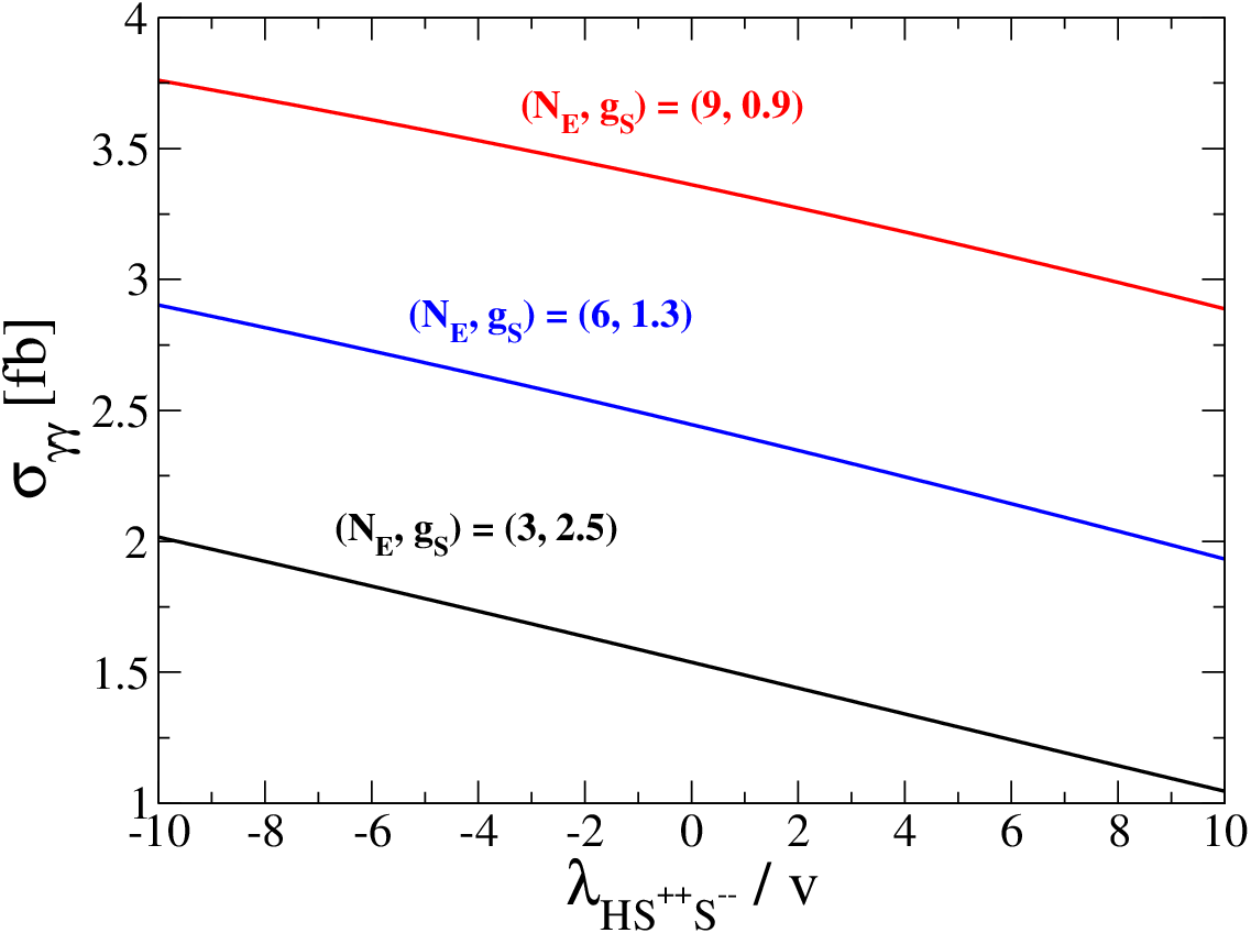
Figure 4: Cross section σγ​γ\sigma_{\gamma\gamma} as a function of λH​S+⁣+​S−⁣−/v\lambda_{HS^{++}S^{--}}/v. We take λH​κ+⁣+​κ−⁣−=λH​S+⁣+​S−⁣−\lambda_{H\kappa^{++}\kappa^{--}}=\lambda_{HS^{++}S^{--}} and λh​κ+⁣+​κ−⁣−=λh​S+⁣+​S−⁣−=0\lambda_{h\kappa^{++}\kappa^{--}}=\lambda_{hS^{++}S^{--}}=0. The black, blue and red curves respectively show the case of (NE,gS)=(3,2.5)(N_{E},g_{S})=(3,2.5), (6,1.3) and (9,0.9). For all the plots, we take sin⁡α=−0.12\sin\alpha=-0.12.

Finally, we add the non-zero contributions to ℋ→γ​γ{\cal H}\to\gamma\gamma from the doubly-charged scalar bosons S±⁣±S^{\pm\pm} and κ±⁣±\kappa^{\pm\pm}. In Fig. 4, we show the diphoton cross section σγ​γ\sigma_{\gamma\gamma} as a function of λH​S+⁣+​S−⁣−(=λH​κ+⁣+​κ−⁣−CLOSE\lambda_{HS^{++}S^{--}}(=\lambda_{H\kappa^{++}\kappa^{--}} normalized by vv in the case of λh​S+⁣+​S−⁣−=λh​κ+⁣+​κ−⁣−\lambda_{hS^{++}S^{--}}=\lambda_{h\kappa^{++}\kappa^{--}}. In this case, only the H→γ​γ/Z​γH\to\gamma\gamma/Z\gamma mode is modified as compared to the previous cases shown in Figs. 2 and 3 for the same parameter choice of NEN_{E} and gSg_{S}. In this figure, we take (NE,gS)=(3,2.5)(N_{E},g_{S})=(3,2.5), (6,1.3) and (9,0.9), and sin⁡α=−0.12\sin\alpha=-0.12 for these three cases, where these points give the maximal allowed value of σγ​γ\sigma_{\gamma\gamma} that is found in Fig. 3. We can see that the constructive effect between the exotic lepton loops and the doubly-charged scalar boson loops is obtained when λh​S+⁣+​S−⁣−<0\lambda_{hS^{++}S^{--}}<0. At λh​S+⁣+​S−⁣−/v=−10\lambda_{hS^{++}S^{--}}/v=-10, we obtain σγ​γ≃2.0\sigma_{\gamma\gamma}\simeq 2.0, 2.8 and 3.8 fb at (NE,gS)=(3,2.5)(N_{E},g_{S})=(3,2.5), (6,1.3) and (9,0.9), respectively.

V Conclusions

We have constructed the three-loop neutrino mass model whose structure is similar to the model by Krauss, Nasri and Trodden. The neutrino masses of 𝒪⁡(0.1){\cal O}(0.1) eV are naturally generated by the loop effect of new particles with their couplings and masses to be of order 0.1-1 and TeV, respectively. We have analyzed the Majorana DM candidate, assuming the lightest of NRN_{R}. The non-relativistic cross section to explain the observed relic density is pp-wave dominant, and there are several processes; NR1​NR1→κ+⁣+​κ−⁣−N_{R}^{1}N_{R}^{1}\to\kappa^{++}\kappa^{--} with the t−t- and u−u-channels, and NR1​NR1→f​f¯N_{R}^{1}N_{R}^{1}\to f\bar{f}, NR1​NR1→Z​ZN_{R}^{1}N_{R}^{1}\to ZZ, NR1​NR1→W+​W−N_{R}^{1}N_{R}^{1}\to W^{+}W^{-}, NR1​NR1→h​hN_{R}^{1}N_{R}^{1}\to hh, NR1​NR1→H​HN_{R}^{1}N_{R}^{1}\to HH with the ss-channel. The dominant DM scattering with a nucleus comes from the Higgs boson mediation hh and HH at the tree level, and we have calculated the spin independent cross section of the process. Furthermore, the anomaly of the muon g−2g-2 can be solved by the one-loop contribution of the triply-charged exotic leptons and doubly-charged scalar boson. We have found the benchmark parameter set to satisfy the relic abundance of the DM, the constraint from the direct search experiment and to compensate the deviation in the measured value of the muon g−2g-2 from the SM prediction.

We then have numerically shown the cross section of the diphoton process via the gluon fusion production g​g→H→γ​γgg\to H\to\gamma\gamma and the width of HH under the constraint from the signal strength μγ​γ\mu_{\gamma\gamma} for the SM-like Higgs boson measured at the LHC Run-I experiment. We have obtained the width to be about 3-5 GeV in the typical parameter region, which gives a tension to the measured value, i.e., about 45 GeV. We have found that the cross section of the diphoton process is given to be a few fb level by taking the masses of new charged fermions and scalar bosons to be 375 GeV with an order 1 coupling constant. A bit larger cross section such as about 4 fb is obtained by taking the larger number of flavor NEN_{E} of the exotic leptons and take a non-zero negative value of the trilinear scalar boson couplings λH​S+⁣+​S−⁣−\lambda_{HS^{++}S^{--}} and λH​κ+⁣+​κ−⁣−\lambda_{H\kappa^{++}\kappa^{--}}.

Acknowledgments

H.O. expresses his sincere gratitude toward all the KIAS members, Korean cordial persons, foods, culture, weather, and all the other things. K.Y. is supported by JSPS postdoctoral fellowships for research abroad.

References

  • [1] ATLAS Collaboration, ATLAS-CONF-2015-081.
  • [2] CMS Collaboration, EXO-PAS-15-004.
  • [3] R. Franceschini et al., arXiv:1512.04933 [hep-ph].
  • [4] S. Moretti and K. Yagyu, arXiv:1512.07462 [hep-ph].
  • [5] S. Di Chiara, L. Marzola and M. Raidal, arXiv:1512.04939 [hep-ph].
  • [6] X. F. Han and L. Wang, arXiv:1512.06587 [hep-ph].
  • [7] A. Angelescu, A. Djouadi and G. Moreau, arXiv:1512.04921 [hep-ph]; R. S. Gupta, S. Jager, Y. Kats, G. Perez and E. Stamou, arXiv:1512.05332 [hep-ph]. D. Becirevic, E. Bertuzzo, O. Sumensari and R. Z. Funchal, arXiv:1512.05623 [hep-ph]; M. Badziak, arXiv:1512.07497 [hep-ph]; N. Bizot, S. Davidson, M. Frigerio and J.-L. Kneur, arXiv:1512.08508 [hep-ph]; A. E. C. Hernández, I. d. M. Varzielas and E. Schumacher, arXiv:1601.00661 [hep-ph]; A. Djouadi, J. Ellis, R. Godbole and J. Quevillon, arXiv:1601.03696 [hep-ph].
  • [8] E. Gabrielli, K. Kannike, B. Mele, M. Raidal, C. Spethmann and H. Veermae, arXiv:1512.05961 [hep-ph]; L. M. Carpenter, R. Colburn and J. Goodman, arXiv:1512.06107 [hep-ph]; R. Ding, L. Huang, T. Li and B. Zhu, arXiv:1512.06560 [hep-ph]; M. x. Luo, K. Wang, T. Xu, L. Zhang and G. Zhu, arXiv:1512.06670 [hep-ph]; T. F. Feng, X. Q. Li, H. B. Zhang and S. M. Zhao, arXiv:1512.06696 [hep-ph]; F. Wang, L. Wu, J. M. Yang and M. Zhang, arXiv:1512.06715 [hep-ph].
  • [9] S. Kanemura, K. Nishiwaki, H. Okada, Y. Orikasa, S. C. Park and R. Watanabe, arXiv:1512.09048 [hep-ph]; T. Nomura and H. Okada, arXiv:1601.00386 [hep-ph]; J. H. Yu, arXiv:1601.02609 [hep-ph]; R. Ding, Z. L. Han, Y. Liao and X. D. Ma, arXiv:1601.02714 [hep-ph]; T. Nomura and H. Okada, arXiv:1601.04516 [hep-ph].
  • [10] L. M. Krauss, S. Nasri and M. Trodden, Phys.  Rev.  D 67, 085002 (2003).
  • [11] M. Aoki, S. Kanemura and O. Seto, Phys.  Rev.  Lett.  102, 051805 (2009); M. Aoki, S. Kanemura and K. Yagyu, Phys. Rev. D 83, 075016 (2011) [arXiv:1102.3412 [hep-ph]].
  • [12] M. Gustafsson, J. M. No and M. A. Rivera, Phys. Rev. Lett. 110, no. 21, 211802 (2013) [Phys. Rev. Lett. 112, no. 25, 259902 (2014)].
  • [13] Y. Kajiyama, H. Okada and K. Yagyu, JHEP 1310, 196 (2013).
  • [14] P. Culjak, K. Kumericki and I. Picek, Phys. Lett. B 744, 237 (2015).
  • [15] H. Okada and K. Yagyu, Phys. Rev. D 93, no. 1, 013004 (2016) [arXiv:1508.01046 [hep-ph]].
  • [16] K. Nishiwaki, H. Okada and Y. Orikasa, Phys. Rev. D 92, no. 9, 093013 (2015) [arXiv:1507.02412 [hep-ph]].
  • [17] S. Kanemura, M. Kikuchi and K. Yagyu, arXiv:1511.06211 [hep-ph].
  • [18] D. Aristizabal Sierra, A. Degee, L. Dorame and M. Hirsch, JHEP 1503, 040 (2015).
  • [19] Y. Farzan, S. Pascoli and M. A. Schmidt, JHEP 1303, 107 (2013).
  • [20] P. A. R. Ade et al. [Planck Collaboration], Astron. Astrophys. 571, A16 (2014).
  • [21] D. S. Akerib et al. [LUX Collaboration], Phys. Rev. Lett. 112, 091303 (2014).
  • [22] F. Jegerlehner and A. Nyffeler, Phys. Rept. 477, 1 (2009).
  • [23] https://twiki.cern.ch/twiki/bin/view/LHCPhysics/CERNYellowReportPageAt1314TeV.
  • [24] G. Passarino and M. J. G. Veltman, Nucl. Phys. B 160, 151 (1979).
  • [25] S. Kanemura, M. Kikuchi and K. Yagyu, Nucl. Phys. B 896, 80 (2015) [arXiv:1502.07716 [hep-ph]].
  • [26] T. Abe, R. Sato and K. Yagyu, JHEP 1507, 064 (2015) [arXiv:1504.07059 [hep-ph]].
  • [27] G. Aad et al. [ATLAS Collaboration], Phys. Rev. D 91, 012006 (2015).
  • [28] V. Khachatryan et al. [CMS Collaboration], Eur. Phys. J. C 75, no. 5, 212 (2015).